


1. Introduction
Policymakers are increasingly concerned with appraising large transport infrastructure proposals comprehensively using rigorous methods (ADB, DFID, JICA and WBG, 2018). Importantly, policymakers are interested in understanding and mitigating the possible negative impact of corridors – such as induced environmental degradation – to maximize their net socioeconomic benefits. In a recent review, Roberts et al. (Reference Roberts, Melecky, Bougna and Xu2020) conclude that large infrastructure investments have been found to increase income and worsen environmental quality. This ‘tradeoff’ between income and environmental quality has rarely been examined in the same setting (study).
This paper evaluates how local income and pollution were impacted by two major highway systems in India: the Golden Quadrilateral (GQ) and North-South-East-West (NSEW) networks. India is a suitable setting for studying this tradeoff because it has invested heavily in large-scale infrastructure projects such as the GQ-NSEW highways, and experienced both rapid economic growth and rising environmental degradation in recent years. Parts of India have some of the highest levels of air pollution in the world (World Bank, 2022). While there is evidence on the GQ's impact on economic activity (Datta, Reference Datta2012; Ghani et al., Reference Ghani, Goswami and Kerr2016), the impacts of these major highway investments on pollution are not as well understood. Rigorously understanding the tradeoffs entailed in such large-scale transport investment projects in settings such as India is also important because of governance issues that raise the cost of road construction (Lehne et al., Reference Lehne, Shapiro and Vanden Eynde2018) and potentially worsen the tradeoff by further lowering the local income gains of such investments.
We use the difference-in-difference (DiD) method, which is increasingly utilized by the literature to estimate the impacts of infrastructure investments (Melo et al., Reference Melo, Graham and Brage-Ardao2013; Redding and Turner, Reference Redding, Turner, Duranton, Vernon Henderson and Strange2015; Berg et al., Reference Berg, Deichmann, Liu and Selod2017; Roberts et al., Reference Roberts, Melecky, Bougna and Xu2020; Alam et al., Reference Alam, Herrera Dappe, Melecky and Goldblatt2022) and has been applied in past studies of the GQ highway (Datta, Reference Datta2012; Ghani et al., Reference Ghani, Goswami and Kerr2016). Unlike before-after comparisons which have traditionally been used in transport project appraisals, this method accounts for the confounding impact of other contemporaneous factors, such as important policy reforms and macroeconomic shocks, by comparing before-after outcomes across locations proximate and distant to the highways. Applying the DiD method to district-level data from 2001 to 2011, we first estimate the impacts the GQ and NSEW highway systems had on district level GDP and environmental quality (particulate matter air pollution and nitrogen dioxide (NO2) levels in the atmosphere). Next, we investigate whether these impacts (and the tradeoffs therein) depended on initial conditions, particularly on educational attainment levels. This is motivated by growing evidence of interactions between transport infrastructure and educational investment in South Asia (Khandker et al., Reference Khandker, Bakht and Koolwal2009; Khandker and Koolwal, Reference Khandker and Koolwal2011; Mukherjee, Reference Mukherjee2012; Aggarwal, Reference Aggarwal2018; Adukia et al., Reference Adukia, Asher and Novosad2020). Much of this evidence base relates to local or rural roads, and hence it is worth examining if national highways also interact with educational investments when affecting key development outcomes.
We find that the improved connectivity due to the GQ highway network had a positive impact on district level per capita GDP. We do not find a similar impact in the case of the NSEW. However, we also find evidence of significant tradeoffs in the GQ impacts: specifically, the highway also increased particulate matter (PM2.5) concentration by 5 per cent. Districts near the GQ highway districts and downwind of them also experienced an increase in particulate matter pollution, a finding consistent with the expected spatial spillover pattern of air pollution due to wind dispersion and recent research on the pollution impacts of rural roads in India (Garg et al., Reference Garg, Jagnani and Pullabhotla2022).
Based on the literature on the health impacts of particulate matter pollution, the implied adverse health and productivity impacts of the pollution caused by the GQ are sizable – for example, equivalent to a 1.25 per cent increase in stunting among children (based on Helf-Neal et al., Reference Helf-Neal, Heger, Vaibhav and Marshall2023) and a 2–3 per cent increase in non-accidental mortality (based on Peters and Pope, Reference Peters and Pope2002; Pope et al., Reference Pope, Burnett, Thun, Calle, Krewski, Ito and Thurston2002).
Regarding the heterogeneity in the highways' impacts, we find that a higher initial rate of educational attainment is associated with a significantly lower air pollution impact of the GQ highway. By contrast, the impact of the GQ on per capita GDP does not vary significantly with the initial rates of educational attainment across districts. Thus, higher skill levels appear to mitigate the income versus air quality tradeoff from highway investments.
We explore one potential mechanism through which higher skills could have mitigated the income versus air quality tradeoff from highway investments: by inducing greater structural transformation toward relatively skill-intensive non-farm activities. We find that the highways prompted a reallocation of labor from farm to non-farm activities. Further, initially higher rates of secondary schooling are associated not just with a less adverse impact of the GQ on air pollution but also with a somewhat greater impact on the reallocation of labor from farm to non-farm activities. Because air pollution has both agricultural and non-agricultural (industrial) sources in India (Kandlikar and Ramachandran, Reference Kandlikar and Ramachandran2000; Pant et al., Reference Pant, Shukla, Kohl, Chow, Watson and Harrison2015; Singhai et al., Reference Singhai, Habib, Raman and Gupta2017; Bikkina et al., Reference Bikkina, Andersson and Kirillova2019), a labor reallocation from farm to non-farm jobs has ambiguous implications for air pollution. However, a reallocation from farm jobs to more skill-intensive non-farm jobs may reduce both agricultural and industrial emissions if more skill-intensive, advanced sectors are less polluting or have better emissions regulation.
We also find that a larger initial share of cropland – a proxy for comparative advantage in agriculture – is associated with a greater impact of the highways on air pollution and a smaller impact on structural change. A larger initial share of cropland may have worsened the income versus air quality tradeoff from highway investments if it limited structural transformation toward more skill-intensive, less polluting non-farm activities. Future research could examine these aspects of the income–environment tradeoff further.
In robustness checks to address concerns about the endogeneity of highway paths, we follow Ghani et al. (Reference Ghani, Goswami and Kerr2016) in using district distances from hypothetical straight-line versions of the highway networks as instrumental variables (IVs) for distances to the actual highways. This approach is now widely used to address the concern that highway routing may be endogenous to local economic prospects (Redding and Turner, Reference Redding, Turner, Duranton, Vernon Henderson and Strange2015); for example, when connecting two nodal points, policymakers may choose to divert the highway from the technically least-cost path toward locations judged to have superior economic prospects, thus biasing estimates of the highway's growth impact upwards. Our results on the impact of the GQ highway on air pollution, the reallocation of jobs from farm to non-farm activities, and the heterogeneity in these impacts based on the initial rates of educational attainment are generally robust to the IV approach; the result on the positive impact on GDP per capita is not. The robustness of the air pollution finding underlines the importance of considering potential tradeoff impacts from highway investments.
Our paper contributes to the evidence base on the tradeoffs between the growth and environmental impacts of transport infrastructure in developing countries. This tradeoff depends not just on how infrastructure affects the overall scale of economic activity, but also on its effects on production techniques and the composition of goods and services (Jayachandran, Reference Jayachandran2022). In the context of India, Asher et al. (Reference Asher, Teevrat and Novosad2020) find that highways caused deforestation. Asher et al. (Reference Asher, Teevrat and Novosad2020) find that rural roads had little to no impact on village income, while Garg et al. (Reference Garg, Jagnani and Pullabhotla2022) find that rural roads increased air pollution by raising labor costs and making it more profitable for farmers to burn agricultural waste instead of employing labor-intensive clearing methods. The tradeoffs between growth and environmental quality may be less stringent in the case of public transportation investments such as railways if they crowd out private vehicles, as suggested by the positive impact of Beijing's subway system on air quality (Li et al., Reference Li, Liu, Purevjav and Yang2019).
Our paper also contributes to the evidence on how the impact of transport investments depends on other policies, institutions, and endowments. Bosker et al. (Reference Bosker, Deichmann and Roberts2015) examine how the impact of China's highways depended on policy restrictions on migration. Michaels (Reference Michaels2008) finds that, as predicted by the Heckscher–Ohlin model, highways in the United States increased the returns to skills in locations with greater skill endowments. Studies have also considered the complementary role of protected area status in mitigating the impacts of road construction on deforestation (Cropper et al., Reference Cropper, Puri, Griffiths, Barbier and Burgess2001; Damania and Wheeler, Reference Damania and Wheeler2015; Dasgupta and Wheeler, Reference Dasgupta and Wheeler2016).
The rest of the paper is organized as follows. Section 2 describes the GQ and NSEW highway systems and the investments in them. Section 3 describes the employed data. Section 4 explains the applied estimation methodology. Section 5 discusses the main estimation results. Section 6 discusses additional estimation results exploring the mechanisms behind the main results and section 7 presents robustness checks. Section 8 discusses the wider socioeconomic implications of the results and section 9 concludes.
2. India's GQ and NSEW highway systems
The GQ is a large-scale highway construction and improvement project connecting India's four top metropolitan cities – Delhi, Mumbai, Chennai, and Kolkata – thereby, forming a quadrilateral. The overall length of the quadrilateral is 5,846 kilometers (km), consisting of four/six-lane express highways. The project was launched in 2001, was about 80 per cent complete by 2005, and was mostly finished in 2007 (Ghani et al., Reference Ghani, Goswami and Kerr2016). The GQ has been found to improve efficiency and output in the manufacturing sector (Datta, Reference Datta2012; Ghani et al., Reference Ghani, Goswami and Kerr2016).
The NSEW project consists of 7,142 km of four/six-lane expressways connecting Srinagar in the north to Kanyakumari in the south, and Silchar in the east to Porbandar in the west. Because of delays associated with land acquisition and zoning permits, only 2 per cent of the work was completed by the end of 2002, and less than 10 per cent by 2005. These figures include the overlapping portions with the GQ network that represent about 40 per cent of the NSEW progress by 2006. Figure 1 highlights the varied temporal context by plotting the degree of completion of the two highway systems over the studied period. While the GQ was nearly 80 per cent complete by the midpoint of our study period (2005), the NSEW reached this level of completion only by the endpoint of our study period (2010).

Figure 1. GQ's and NSEW's degree of completion over time.
Source: Authors, based on NHAI data.
3. Data
We use a district-level panel dataset to estimate the impact of the highways. Districts are the primary administrative units of India below the state level. In the last year in our data set, 2010–11, there were about 640 districts in India.
Our main source for the district-level data is the South Asia Spatial Database, a database compiled by the World Bank's Office of the Chief Economist for South Asia using official censuses and surveys, administrative records, surveys, satellite imagery, and official maps. We use it to construct a district-level panel for two years, 2000–01 and 2010–11.
Table A1 in the online appendix lists the main outcome variables used in our study and summarizes them for 2001 and 2011. The measure of local income is district-level per capita GDP, which is published by the Directorate of Economics and Statistics, the Planning Commission, Government of India. The measures of environmental quality relate to particulate matter (PM) or aerosols in the air – as measured by aerosol optical thickness (AOT) – as well as measures of NO2 air pollution. These variables are annual averages of monthly observations sourced from NASA Earth Observations. Our measures of the structure of employment – the share of farm and non-farm jobs in total employment – are based on the 2001 and 2010 Population Censuses of India, conducted in 2001 and 2011.
AOT is a satellite-based measure of the ‘thickness’ of PM in the atmosphere. Specifically, it is the degree to which aerosols prevent the transmission of light by absorbing or scattering light. An optical thickness of less than 0.1 indicates a crystal-clear sky with maximum visibility, whereas a value of 1 indicates the presence of aerosols so dense that people would have difficulty seeing the sun. We choose AOT as a measure of air pollution because rising levels of PM air pollution and its health impact are a major concern in India, and because researchers are increasingly using satellite-based AOT to track air quality in low and middle incomes countries in the absence of other air pollution data in high spatial–temporal resolutions (Kumar et al., Reference Kumar, Chu and Foster2007). There is a strong correlation between AOT from satellite data and ground measurements of PM (Kaufman et al., Reference Kaufman, Dubovik, Smirnov and Holben2002; Li et al., Reference Li, Lau, Mao and Chu2005; Chu, Reference Chu2006; Kumar et al., Reference Kumar, Chu and Foster2007). The sources of PM in South Asia are understood to include human activities, particularly vehicular emissions, industrial emissions, fuel use for domestic purposes such as cooking, and the burning of crops and household wastes (Kandlikar and Ramachandran, Reference Kandlikar and Ramachandran2000; Pant et al., Reference Pant, Shukla, Kohl, Chow, Watson and Harrison2015; Singhai et al., Reference Singhai, Habib, Raman and Gupta2017).
NO2 is a growing air pollutant in (urban) South Asia, with severe health impacts and a role in producing other secondary pollutants such as ozone and acid rain (Ul-Haq et al., Reference Ul-Haq, Tariq and Ali2015; Aggarwal and Toshniwal, Reference Aggarwal and Toshniwal2019). It is emitted mainly from burning fossil fuels for transportation and electricity generation. From 2005 to 2014, its levels increased by more than 20 per cent in the major Indian cities of Chennai, Bengaluru, and Kolkata (NASA Earth Observatory, 2016).
Our main initial condition variable for the heterogenous impact analysis, which measures district-level educational attainment, is the secondary school completion rate: that is, the percentage of individuals aged 15 years and above who had attained secondary school or a higher educational level as of 2001. We also examine the heterogeneity in impact with respect to the share of cropland in the total area of the district, a proxy for comparative advantage in agriculture. Table A2 (online appendix) presents summary statistics of the variables.
Many Indian districts were renamed or subdivided during our study period, in large part due to the creation of three new states between 1999 and 2002. Thus, there were a total of 640 districts recorded in the 2011 Census of India as opposed to 593 in the 2001 Census of India. We harmonized district boundaries over time by mapping newly created districts back to their unique parent district in 1999. For instance, if district X in 1999 was split into districts Y and Z by 2010, we combine the 2010 data for Y and Z to recreate the parent district X in 2010. In addition to aggregating new districts to their 1999 parent district, we have dropped districts from the remote states of Jammu and Kashmir and northeastern India from our analysis. This is standard practice in district-level studies on India, including previous studies on the impact of the GQ highway. After these steps, our data set consists of 427 consistently defined districts per year.
3.1 Measures of distance from the GQ and NSEW highways
We have merged geo-coded data on the location of the GQ and NSEW networks into the district database.Footnote 1 This information is used to calculate the distances of district centroids (the geographic center of the district area) from the nearest points on the GQ and NSEW networks. Figure 2 plots the highway networks (excluding parts of NSEW that were not built by 2010) and the distance of every district centroid from its nearest point on each highway. We also categorize districts into four distance bands from each highway: nodal (major metropolitan area at which the highways start and end),Footnote 2 0–40 km from the highway, 40–100 km from the highway, and more than 100 km from the highway.Footnote 3 Thus, there are eight distance bands in total.

Figure 2. GQ and NSEW highway networks, with distances from district centroids. (a) Golden Quadrilateral (GQ). (b) North-South-East-West Highway.
Notes: GQ = Golden Quadrilateral; NSEW = North-South-East-West Highway. The green lines depict the shortest distance from district centroids (blue dots) to the actual highway placement (red lines).
Table A4 in the online appendix shows the distribution of districts across these distance bands. As explained later in the methodology section, we use these bands to assign districts to the ‘treatment’ and ‘control’ groups in the DiD estimation. Specifically, the 0–40 km distance band from the GQ (or the NSEW) identifies the GQ (or NSEW) treatment districts, while the control districts are those more than 100 km away from both highways. Table A4 therefore shows that our sample contains 72 GQ treatment districts and 40 NSEW treatment districts. There are 194 districts in the common control group. There is little overlap between districts proximate to GQ and those proximate to NSEW; it would be difficult to distinguish between the impacts of these highways were this not the case.
Figure A1 in the online appendix depicts hypothetical straight-line versions of the GQ and NSEW highways used in robustness checks. The nodal cities used to construct the straight-line version of the GQ are Delhi, Kolkata, Chennai, Bangalore, and Mumbai. The nodes used to construct the NSEW straight-line versions are cities at its northern, western, and southern extremities (Jalandhar, Porbandar, and Kanniakumari, respectively), and Jhansi in central India (where the East-West and North-South arms of the NSEW cross). We ignore the arm of NSEW going east from Jhansi because it was largely unbuilt in 2010.Footnote 4
Table A5 (online appendix) shows the distribution of districts according to their distance bands from the actual versus straight line versions of GQ and NSEW. In general, there is a strong but less than a perfect overlap in these distributions.
4. Estimation methodology
We use the DiD methodology to estimate the impact of the highways on district-level outcomes of interest. This method compares the change in the outcome of interest after the highway was built in districts located close to the new highways (the treatment districts) to those located far from them (the control districts). The first differencing – that is, looking at the change in the outcome after highway construction – controls for the confounding effect of unobserved factors that do not change over time. For instance, districts that are near the highways could have been relatively productive even before the highways were built. The second differencing – that is, comparing the change across treatment and control districts – controls for the confounding effect of unobserved factors common to control and treatment districts that do vary over time, such as macro shocks and national policy changes. The key identifying assumption is that the treatment districts have similar trends to the control districts in the absence of treatment.
4.1 Estimating the average impacts of the highways
Formally, the underlying regression specification can be described as follows:

This regression is estimated on district-level panel data. Here, Yi,t is an outcome of interest in district i and year t. The dummy variable $\textrm{Post}_t^{\textrm{Highway}}$ is equal to one in years after the highway completion, and zero in years prior to that. The dummy variable $\textrm{Highwa}{\textrm{y}_i}$
 is equal to one in districts close to the new highways (the treatment districts) and zero otherwise. ${\emptyset _i}$
 is a set of district fixed effects that controls for time-invariant district-level factors, and ${\varphi _t}$
 is a set of year dummies that control for unobserved time-varying factors common to all districts. The impact of the highways is estimated by $\beta$
 , the coefficient on the treatment variable (the interaction $\textrm{Highwa}{\textrm{y}_i} \times \textrm{Post}_t^{\textrm{Highway}}$
 ), which measures how the change in the outcome after the highway was built differed across control and treatment districts.
We adjust this basic specification to account for the fact that we are simultaneously estimating the impacts of two highway networks, the GQ and the NSEW. There are two factors to consider in this regard. First, in estimating the impact of either highway network, it is important to control for the presence of the other one. Second, the two networks could have had different impacts. In other words, there were two sets of treatment districts: those near GQ, and those near NSEW.
We assign districts into distance bands based on the proximity of the district centroid to the GQ. The bands are: more than 100 km from the nearest GQ point, 40–100 km from the GQ, 0–40 km from the GQ, and nodal districts.Footnote 5 We then interact the indicators for each GQ distance band with a variable indicating the years after the GQ was built. We repeat this process for the NSEW and include both sets of interactions on the RHS. Thus, the specification we estimate is as follows:

here, $\textrm{G}{\textrm{Q}_i}$ (respectively, $\textrm{NSE}{\textrm{W}_i}$
 ) is a vector of dummies indicating the distance band from the GQ (respectively, NSEW) to which district i belongs, while $\textrm{Post}_t^{\textrm{GQ}}$
 (respectively, $\textrm{Post}_t^{\textrm{NSEW}}$
 ) is a dummy equal to one in the years after GQ (respectively, NSEW) completion. The omitted distance band dummy corresponds to districts more than 100 km from the highway (GQ or NSEW). ${\emptyset _i}$
 is a set of district fixed effects, and ${\varphi _t}$
 is a set of year dummies (or state-year dummies).
Because GQ and NSEW construction commenced after 2001, the indicators $\textrm{Post}_t^{\textrm{GQ}}$ and $\textrm{Post}_t^{\textrm{NSEW}}$
 are set equal to zero in the baseline year of our two-period panel (2000–01) and one in the endline year (2010–11). To account for the fact that, unlike GQ, NSEW was not fully completed by 2010–11, only those segments of NSEW that were complete as of 2010 are considered when assigning districts to distance bands around NSEW.
The impact of the GQ is measured by the ${\beta ^{\textrm{GQ}}}$ corresponding to the 0–40 km distance band from GQ, to be denoted by ${\beta ^{\textrm{GQ}, 0 - 40 }}$
 hereafter. Because we are controlling for $\textrm{NSE}{\textrm{W}_i} \times \textrm{Post}_t^{\textrm{NSEW}},{\beta ^{\textrm{GQ,}0 - 40}}$
 in effect measures how the post-GQ change in the outcome differed between districts 0–40 km from GQ (the GQ treatment group) and districts more than 100 km from both highways (the control group). Similarly, the impact of NSEW is measured by the ${\beta ^{\textrm{NSEW}}}$
 , corresponding to the 0–40 distance band from the NSEW, denoted by ${\beta ^{\textrm{NSEW}, 0 - 40 }}.$
 Our main results tables thus report these two $\beta$
 s.
s.
In our specification, we use flexible state-year fixed effects instead of a common year fixed effect. This preferred specification controls for unobserved state-level differences in growth – to account for the documented divergence in economic growth across Indian states (GOI, 2017).
4.2 Estimating conditional impacts: could highway impacts have depended on local market conditions such as initial education levels?
We also test the hypotheses that the impact of the highways depended on initial conditions in districts, focusing on the initial rates of educational attainment in the district. Roberts et al. (Reference Roberts, Melecky, Bougna and Xu2020) and Alam et al. (Reference Alam, Herrera Dappe, Melecky and Goldblatt2022) use a simple policy model to argue that gaining a greater understanding of the heterogenous (or ‘conditional’) impacts of transport corridor investments – including highways – is needed to better inform policy decisions on the design of corridor investment programs. However, they also document that attempts to estimate heterogenous impacts of connectivity are scarce in the literature.
Our regression estimation thus exploits the information on varying initial conditions across districts and adopts a difference-in-difference-in-difference approach by interacting the treatment variable $(\textrm{Highwa}{\textrm{y}_i} \times \textrm{Post}_t^{\textrm{Highway}})$ with variable(s) capturing initial conditions in districts:

here, ${Z_{i }}$ is a vector of initial conditions of interest in district i. The effect of initial conditions on the impact of the highways is estimated by the $\delta$
 s, the coefficients on the triple interaction term between $\textrm{Highwa}{\textrm{y}_i} \times \textrm{Post}_t^{\textrm{Highway}}$
 and the ${Z_{i }}$
 s.
s.
For illustration, suppose that the ${Z_{i }}$ in question is a variable measuring initial rates of educational attainment. The corresponding ${\delta ^{\textrm{GQ}}}$
 (respectively, ${\delta ^{\textrm{NSEW}}}$
 ) coefficient measures how the impact of the GQ (respectively, the NSEW) depends on the local level of educational attainment. A positive estimate of this ${\delta ^{\textrm{GQ}}}$
 would imply that the impact of the GQ on the outcomes of interest was more positive in districts with higher initial rates of educational attainment.
4.3 Examining robustness to endogenous highway route: two-stage least squares estimation using instrumental variables
Ordinary least squares (OLS) estimates of the highway impacts could be biased if the placement of the highways was correlated with unobserved factors affecting local developmental outcomes. For example, it could be that the path of the highways was deliberately tilted toward locations with good growth prospects. Datta (Reference Datta2012) argues that such endogenous placement is not a major concern with the GQ and NSEW projects because they were largely highway upgrade projects and, as such, their routes were pre-determined by existing highway segments. While we agree with this reasoning, there remains a concern that in parts of the highway networks, there was room to choose between alternative pre-existing segments.
As in Ghani et al. (Reference Ghani, Goswami and Kerr2016), we address this concern by employing a two-stage least squares (2SLS) estimation strategy using IVs as a robustness check. To qualify as an instrument, a variable must be correlated with the treatment variable but uncorrelated with unobserved factors affecting the outcomes being considered. Because the highways were intended to connect certain pre-specified nodal cities, the straight-line paths connecting those nodes are close to the actual paths of the highways while arguably being exogenous to unobserved drivers of developmental outcomes in non-nodal districts. Hence, our chosen IVs measure district proximity to hypothetical straight-line versions of the GQ and NSEW highways.
For illustration, consider the hypothetical straight-line version of the GQ, constructed by replacing each highway segment connecting a pair of GQ nodal cities with the straight line joining those nodes. We generate a dummy variable indicating districts whose centroids are within 40 km of this hypothetical highway network. The interaction of this variable with $\textrm{Post}_t^{\textrm{GQ}}$ instruments for the GQ treatment variable (that is, it instruments for the interaction of $\textrm{Post}_t^{\textrm{GQ}}$
 with a dummy indicating that the district is within 0–40 km of the actual GQ). A similar procedure generates the IV for the NSEW treatment variable.
5. Main results
5.1 Average wider economic impacts of the highways
Table 1 reports the estimation results for equation (2), our baseline DiD specification measuring the average impact of the highways. In line with prior research on the impact of the GQ on industrial activity (Ghani et al., Reference Ghani, Goswami and Kerr2016), the estimation results suggest that the GQ highway had a statistically significant positive impact on district output per capita. Looking at column (1) of table 1 with the results for GDP per capita (in logs), the point estimate of ${\beta ^{\textrm{GQ}, 0 - 40 }}$ implies that the highway increased GDP per capita by about 4 per cent.
Table 1. Impacts of highways on income and environmental quality

Notes: The OLS estimation is based on four distance bands on the proximity of district centroid to highways (0–40 km, 40–100 km, more than 100 km, and nodal districts) interacted with post-treatments. The omitted (comparator) distance bands are those exceeding 100 km. Only the coefficients on the 0–40 km distance bands are shown for conciseness. Standard errors clustered by district in parentheses.
As for the highways' impacts on environmental measures (table 1, columns (3) and (4)), it appears that the GQ highway led to an increase in air pollution related to PM. Specifically, the GQ is estimated to have increased AOT by approximately 0.03 points. When compared to the mean increase of AOT (0.07 points) across all districts during this period, this impact is highly significant in magnitude. We do not detect a significant impact on NO2 levels in the air in the districts in the vicinity to the GQ highway (0–40 km).
Because wind disperses particulates in the air, air pollution could have also increased downwind of the highway. To examine this, we first determine the annual average downwind direction for each GQ (0–40) district by analyzing the hourly wind dataset obtained from the European Center for Medium-Range Weather Forecasts' Climate Data Store. Utilizing the u- and v-components of the wind at various locations within a district, we find the median wind angle over the course of a year and average it for the years 2000 and 2001. The wind angle at the district level remains highly consistent from year to year, exhibiting a correlation exceeding 0.9 between both years.
We then group the GQ (40–100) districts into two categories: (i) ‘downwind districts’ are those whose centroid direction from a nearby GQ (0–40) district is within 45 degrees of the wind direction of that GQ district; and (ii) ‘near GQ districts’ are the remaining districts in the GQ (40–100) group. Online appendix table A6 shows that, compared to the control districts (those far away from GQ and NSEW, as in the rest of our estimations), there was a statistically significant increase in particulate matter pollution in districts near and downwind of GQ districts (the coefficient on Post GQ* Downwind in column (2)), but not in other districts near GQ districts (the coefficient on Post GQ* Near in column (2)). We do not observe a similar downwind impact on GDP. Hence, this result indicates that, because PM disperses in the air, ignoring downwind districts may be missing the environmental spillover of the GQ on nearby districts. It suggests that the GQ's positive impact on income was more geographically concentrated than its negative impact on environmental quality. Moreover, this pattern of spillovers also serves as a robustness check on our main result: if our result is spuriously driven by some unobserved factor that happens to be spatially correlated with GQ, then we would not expect its spatial spillovers to depend on wind direction specifically from the GQ district.
Overall, these average findings raise a question of whether some measures or local market conditions could be identified to mitigate the tradeoff between income growth and worsening air pollution. We focus on this important question next.
5.2 Heterogenous impacts: can human capital help mitigate the income–environment tradeoff?
To examine heterogeneity in the highways' impact, we estimate the triple-difference specification in equation (3) by OLS. Recall that we are interested in estimating the coefficients on the interactions between the treatment $(\textrm{Highwa}{\textrm{y}_i} \times \textrm{Post}_t^{\textrm{Highway}})$ and variables ${Z_i}$
 that capture the initial conditions. Our broad hypothesis is that, as predicted by a Heckscher–Ohlin type model of comparative advantage and trade, the impact of better market access may depend on certain factor endowments such as educational attainment and cropland (which are immobile in the short to medium term). If this is correct, then low average levels of factor endowments could explain why the average district may not experience wider economic benefits and incur wider economic costs from the highway construction. From the policymaker's perspective, identifying such complementary factors can reveal how the highway investment programs could be enriched with complementary public interventions to maximize the wider economic benefits and mitigate the wider economic cost generated by these investments.
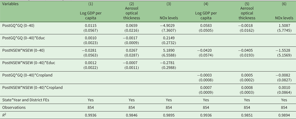
The estimation results in table 2 first consider the interactions of highway with educational attainment, as measured by the secondary school completion rate (the variable Educ). No statistically significant heterogeneity impact of connectivity on GDP per capita is found depending on the secondary school completion rate: the coefficient on the triple interaction terms with Educ is statistically not significant (table 2, column (1)).Footnote 6 By contrast, for the PM air pollution (measured by AOT), the coefficient on the interaction of PostGQ*GQ (0–40) with Educ is negative and statistically significant at the 5 per cent level (table 2, column (2)). This finding suggests that higher educational attainment mitigated the increase in PM air pollution caused by the GQ. The magnitude of this heterogeneity is sizable, with the estimate implying that moving from a district at the 25th percentile of the secondary school completion rate (17 per cent) to one at its 75th percentile (29 per cent) would reduce the impact of the GQ on AOT by 0.02 percentage points (compared with the average AOT impact of 0.06 points shown in table 1, column (2)).
Table 2. Heterogenous Impacts of highways
Notes: The OLS estimation is based on four distance bands on the proximity of district centroid to highways (0–40 km, 40–100 km, more than 100 km, and nodal districts) interacted with post-treatments. Only the coefficients on the 0–40 km distance bands are shown for conciseness. The omitted (comparator) distance bands are those exceeding 100 km. Standard errors in parentheses. Standard errors are clustered at the district-level.
Next, we include an interaction of the highway treatment variables with a measure of the share of cultivated land in the total district area (the variable Cropland). We are interested in this interaction term because the impact of the highways could also depend on the comparative advantage in agriculture (proxied by Cropland).
Interestingly, for the AOT outcome variable (table 2, column (5)), the coefficients on the interactions of PostNSEW*NSEW(0–40) and PostGQ*GQ (0–40) with Cropland are positive and statistically significant at the 1 and 10 per cent levels, respectively. These estimates indicate that the income–air pollution tradeoff was worse in more agricultural districts.
6. Exploring the transmission channels behind the heterogenous impacts: a structural change
The results in section 5.2 suggest that districts with initially higher educational attainment were subject to a less severe income–pollution tradeoff from the GQ, while those with a higher initial share of agricultural land experienced a more severe income–pollution tradeoff. A potential explanation for these findings is that patterns of comparative advantage – as proxied by baseline Educ and Cropland – caused districts to specialize in activities involving different income–air pollution tradeoffs after the GQ or NSEW reduced the trade costs between them. We explore these hypotheses by considering the heterogenous impacts of the highways on the structural transformation of employment.
Our analysis indicates that, on average, both the GQ and the NSEW increased the share of non-farm jobs in total employment (table 3, column (1)). For example, according to the point estimate of ${\beta ^{\textrm{GQ}, 0 - 40 }}$ in table 3, column (1), which is statistically significant at the 10 per cent level, the GQ highway increased the share of non-farm employment by 1.6 percentage points. This is a big impact because the baseline increase in the share of non-farm employment in control districts during this period was 2.5 percentage points. The estimate of ${\beta ^{\textrm{NSEW}, 0 - 40 }}$
 too is positive and statistically significant. Specifically, the NSEW highway appears to have raised the share of non-farm employment by about 2.5 percentage points.
Table 3. Impacts of highways on non-farm employment

Notes: The OLS estimation is based on four distance bands on the proximity of district centroid to highways (0–40 km, 40–100 km, more than 100 km, and nodal districts) interacted with post-treatments. Only the coefficients on the 0–40 km distance bands are shown for conciseness. The coefficients on the interactions of Post with Cropland and Education are not shown for conciseness. The omitted (comparator) distance bands are those exceeding 100 km. Standard errors clustered by district in parentheses.
We do not find any significant impact of the highways on the total population and the total employment rate of the population (as measured by the Census), suggesting that the highways did not bring additional labor into the district economies and only changed the farm and non-farm composition of total employment.Footnote 7
Next, we find that the GQ impact on structural change varied significantly with the initial rates of higher educational attainment. Specifically, considering the share of non-farm employment as an outcome, the coefficient on the interaction of PostGQ*GQ (0–40) with Educ is positive and statistically significant at the 10 per cent level (table 3, column (2)). Hence, districts with initially higher rates of educational attainment experienced somewhat greater structural transformation after the GQ completion.
For the NSEW, we find that its impact on structural change was lower in areas with a higher initial share of cropland. Specifically, considering the share of non-farm employment as an outcome, the coefficient on the interaction of PostNSEW*NSEW (0–40) with Cropland is negative and statistically significant at the 10 per cent level (table 3, column (3)).
A potential explanation for these patterns is that initially higher rates of educational attainment may have mitigated the income versus air quality tradeoff from highway investments by inducing greater structural transformation toward more skill-intensive non-farm activities that emit less air pollution. In contrast, a larger share of cropland may have exacerbated the income versus air quality tradeoff from highway investments by limiting structural transformation toward more skill-intensive non-farm activities, and maintaining or increasing farm activities (which are associated with crop burning, a major source of air pollution in India).
7. Robustness to endogenous placement of highways: 2SLS (IV) estimates
As explained in section 4.3, we test for the robustness to endogenous highway placement using the interaction of $\textrm{Post}_t^{\textrm{GQ}}$ (respectively, $\textrm{Post}_t^{\textrm{NSEW}}$
 ) with a dummy for the district being within 40 km of the hypothetical straight-line version of GQ (respectively, NSEW) as the IV for PostGQ*GQ (0–40) (respectively, PostNSEW*NSEW (0–40)).Footnote 8
Table A7 in the online appendix presents the first stage results of the 2SLS estimation strategy. Considering PostGQ*GQ (0–40) as the outcome variable (column (1)), the coefficient on the interaction of $\textrm{Post}_t^{\textrm{GQ}}$ with the dummy for the 0–40 km distance band from the straight-line GQ highway is positive and significant at the 1 per cent level. Similarly, considering PostNSEW*NSEW (0–40) as the outcome variable (column (2)), the coefficient on the interaction of $\textrm{Post}_t^{\textrm{NSEW}}$
 with the dummy for the 0–40 km distance band from the straight line NSEW highway is positive and significant at the 1 per cent level.
Table A8 (online appendix) presents the 2SLS estimates of the impact of the highways on income and air pollution. For GDP per capita as the outcome (column (1)), the 2SLS coefficient on the GQ treatment variable is lower than the corresponding OLS estimate and no longer statistically significant, suggesting that the OLS estimate was biased upwards due to endogenous placement near locations with better economic prospects. For AOT as the outcome (column (2)), the 2SLS coefficient on the GQ treatment variable is 0.04, and significant at the 1 per cent level (the corresponding OLS estimate was 0.03). Therefore, our finding about the impact of the GQ on PM pollution is robust to the IV strategy.
Table A9 in the online appendix presents the 2SLS estimates for the heterogenous impacts of the GQ and NSEW highways. The results are similar to the OLS results presented in table 3. They indicate that the impact of the GQ on PM air pollution was significantly lower in locations with initially higher rates of educational attainment (column (2)), and it was significantly greater in locations with more cropland (column (5)).
Table A10 (online appendix) presents the 2SLS estimates for the impacts of the highways on structural change in employment. The results regarding the average impact on non-farm employment are similar to the OLS results. Regarding the heterogenous impacts on non-farm employment with respect to the initial rates of education and cropland, while the signs of the estimated coefficients are consistent with OLS results, they are not statistically significant.
In addition, an alternative measure of local economic activity using nightlights would make our findings more replicable in other contexts because it is more widely available than district-level GDP. Therefore, we also generate results using nightlights measure in place of district-level GDP and report them in online appendix table A11. The results are consistent with our GDP results in the case of nightlights intensity per unit area, but they are inconclusive when using nightlights intensity per capita as the outcome variable.Footnote 9
Finally, we explore why GQ is found to have impacts but NSEW is not. It could be due to the shorter gestation lag at which we estimate the effect for the NSEW compared with the GQ – which was completed earlier (see figure 1). To corroborate this explanation, we estimated the effect of GQ and NSEW in 2005. Consistent with the gestation lag hypothesis, the OLS estimate of the impact of GQ for the intermediate year of 2005 is statistically significant but smaller in magnitude than that for 2011, while the corresponding IV estimate is statistically not significant (table A12 in the online appendix). Similarly, we do not find a significant impact of the GQ on the log GDP per capita of districts in the intermediate year of 2005 (table A13, online appendix).Footnote 10 Another possible explanation is that the district-level effects of NSEW have been much more heterogenous, possibly depending on local initial conditions that could have varied in type across districts.
8. Wider socioeconomic impacts of pollution from highways
To better understand how the highways affected health and productivity, we combine our coefficient estimates with estimates of health and productivity impacts from the literature. Note that, due to data limitations, our study uses AOT, a satellite-based measure of PM pollution, whereas most of the relevant epidemiological literature uses ambient PM2.5 concentration as a measure of PM pollution. Hence, we need to convert AOT to PM2.5 concentration to simulate health impacts. According to our baseline OLS specification, the GQ highway increased AOT by 0.03, or 10 per cent of the mean AOT in Indian districts. Based on a study of the empirical relationship between AOT and ground-based measures of ambient P52.5 concentrations in India (Kumar et al., Reference Kumar, Chu and Foster2007), this translates into a 5 per cent increase in the concentration of PM2.5 caused by the GQ.
The implied health impact of the increased air pollution is significant. For example, a 5 per cent increase in PM2.5 is associated with a 1.25 per cent increase in stunting among children (Helf-Neal et al., Reference Helf-Neal, Heger, Vaibhav and Marshall2023) and a 2–3 per cent increase in non-accidental mortality (Peters and Pope, Reference Peters and Pope2002; Pope et al., Reference Pope, Burnett, Thun, Calle, Krewski, Ito and Thurston2002). Based on a study in Kanpur district of India, a 5 per cent increase in PM2.5 would increase annual per capita health expenditure by USD0.62 (Gupta, Reference Gupta2008). Given the total population of all GQ affected districts in 2011, this amounts to a total additional health expenditure of USD157 million per year (about 4 per cent of the cumulative GQ construction cost of USD3.9 billion in 2011). To put this in perspective, suppose an annual tax of USD157 million is imposed to account for the health externality. Assuming a planning horizon of 25 years and a discount rate of 10 per cent, the net present value of this externality tax would equal about 40 per cent of the cumulative GQ construction cost. An alternate estimate from China implies a 15 per cent increase in annual health expenditure due to the pollution from GQ (Yang and Zhang, Reference Yang and Zhang2018).
The implied adverse productivity impacts are significant too. Based on a recent estimate from China, a 5 per cent increase in PM2.5 would reduce output per worker in manufacturing firms by 2.2 per cent (Fu et al., Reference Fu, Viard and Zhang2021).
9. Conclusion
This paper studied the potential income–environment tradeoff in wider economic impacts of transport corridor investments in the case of India's GQ and NSEW highways. This potential tradeoff has been highlighted in the literature (Roberts et al., Reference Roberts, Melecky, Bougna and Xu2020) but not studied under one case.
Our findings confirm the existence of the income–environment tradeoff in the case of India's highway programs. The GQ highway increased the growth of GDP per capita over 2001–11 by 4 percentage points in connected districts over the baseline of 27 per cent growth in control districts. For NSEW, the average estimated impact is also positive but statistically insignificant – likely because of the shorter gestation lag since the NSEW was completed. In tandem, the GQ highway significantly increased ‘aerosol optical thickness,’ a measure of particulate air pollution, by 0.03 points, relative to the baseline increase of 0.07 point over the study period. Moreover, the income boost was more geographically concentrated than the degradation of environmental quality which extended further from the highway corridor and into downwind districts near the highways.
Examining the heterogeneity in these highway impacts, we focused on the potential role of initial rates of education attainment and found that the adverse impact of the GQ on particulate matter air pollution was weaker in districts with initially higher shares of local population with completed secondary schooling. Additionally, it was stronger in districts with a higher share of cropland in total land area.
These heterogenous impacts could be related to the structural changes induced by the highway. On average, we find that both highways have induced a structural change in employment by increasing the share of non-farm jobs – but not increasing total employment. This impact on structural change is greater in districts with a comparative advantage in skill-intensive non-farm activities (proxied by initial rates of secondary schooling) and lower in districts with a comparative advantage in farm activities (proxied by initial cropland shares). Overall, these patterns suggest that locations with a comparative advantage in skill-intensive non-farm activities and a comparative disadvantage in farm activities have experienced an income–pollution tradeoff from the highways that is less harsh.
The mechanisms behind this pattern could be examined in future research, as it has potentially important policy implications. Systematically increasing rates of educational attainment alongside connectivity interventions – such as incorporating place-based skilling projects into a broader corridor investment program – could help ensure that wider economic impacts of highways across income and environmental quality generate significant synergies.
From the policy perspective of choosing how much to invest in highway networks versus substitutes for them, it is worth considering whether the income–pollution tradeoff is lower in case of railroads. However, it is difficult to compare the relative cost–benefits of rails and highways based on our findings, and future research could focus on comparing the income–pollution tradeoffs for highways versus railroads.
Supplementary material
The supplementary material for this article can be found at https://doi.org/10.1017/S1355770X23000177.
Acknowledgements
The authors thank Sarur Chaudhary and Ruifan Shi for their excellent research support. They thank Martin Rama, Marianne Fay, William Maloney, Uwe Deichmann, Somik Lall, Yasuyuki Sawada, Arjun Goswami, Jay Menon, Akio Okamura, Takayuki Urade, Duncan Overfield and two anonymous referees for helpful suggestions. The findings, interpretations, and conclusions expressed in this paper are entirely those of the authors and do not necessarily represent the views of the World Bank, its Executive Directors, or the governments of the countries they represent. Melecky acknowledges support from the Czech Science Foundation ‘19-19485S–Spatial Dynamics and Inequality: The Role of Connectivity and Access to Finance.’
Competing interests
The authors declare none.


