


1. Introduction
Barnett (Reference Barnett1980) developed Divisia monetary aggregates as an alternative to conventional simple sum monetary aggregates, which are only meaningful economic aggregates if the components of the aggregate are “perfect substitutes in identical ratios” over the sample; see also Barnett (Reference Barnett1982) and Barnett et al. (Reference Barnett, Fisher and Serletis1992). As Belongia (Reference Belongia1996) explained, simple sum aggregates cannot internalize pure substitution effects unless perfect substitution holds, which in turn would imply that all pairwise elasticities of substitution between the components are infinite—an assumption that is strongly rejected empirically. Morishima elasticities of substitution between monetary assets can be estimated from money demand systems and are frequently used to assess the validity of conventional monetary aggregates vis a vis Divisia aggregates; see, for example, Fisher and Fleissig (Reference Fisher and Fleissig1997), Drake et al. (Reference Drake, Fleissig and Swofford2003), Jin (Reference Jin2016), Barnett and Gaekwad (Reference Barnett and Gaekwad2018), Chang and Serletis (Reference Chang and Serletis2019), Jadidzadeh and Serletis (Reference Jadidzadeh and Serletis2019), and Xu and Serletis (Reference Xu and Serletis2022).Footnote 1
Xu and Serletis (Reference Xu and Serletis2022) argue that low elasticities of substitution between monetary assets imply that “velocity is easy to predict, and the central bank can target key monetary aggregates to accommodate the demand for money and near monies and affect general macroeconomic variations.” Following this line of reasoning, low elasticities of substitution between monetary assets would imply that Divisia monetary aggregates could play a role in the conduct of monetary policy, but that simple sum aggregates would not be reliable money measures. In this paper, we estimate elasticities of substitution between components of the Bank of England’s UK household-sector Divisia monetary aggregate and analyze their policy implications from 1999 up to 2019, which encompasses the period surrounding the global financial crisis but does not include the COVID-19 pandemic.
Divisia monetary aggregates have been frequently used in economic analysis. Ghosh and Parab (Reference Ghosh and Parab2019), for example, analyze the time-varying correlation between money growth and industrial production in a GARCH framework using both Divisia aggregates and conventional monetary aggregates for the UK and other countries with their results favoring the use of Divisia measures. Ghosh and Bhaduri (Reference Ghosh and Bhaduri2018) consider the relationship between Divisia measures and exchange rates for the UK and other countries emphasizing the zero lower bound on interest rates. In the context of the global financial crisis, Rayton and Pavlyk (Reference Rayton and Pavlyk2010) illustrated a “recent decoupling” beginning in mid-2008 between the Bank of England’s Divisia M4 aggregate and the corresponding simple sum M4 aggregate. Bissoondeeal et al. (Reference Bissoondeeal, Karogloua and Binner2019) test whether real money growth affects the output gap for the UK using Divisia and simple sum M4 and find stronger results for Divisia M4; see also Elger et al. (Reference Elger, Jones, Edgerton and Binner2008). A key finding of our study is that for UK household-sector monetary assets substitution is generally inelastic in response to changes in the user cost of noninterest-bearing assets and, consequently, simple sum aggregates are poor indicators of monetary conditions for the UK relative to Divisia aggregates. Following Xu and Serletis (Reference Xu and Serletis2022), our results also suggest a role for Divisia monetary aggregates in the conduct of monetary policy for the UK, since the estimated substitution elasticities are low on at least some dimensions. More generally, Brill et al. (Reference Brill, Nautz and Sieckmann2021) highlight the increasing relevance of monetary aggregates in the period of low interest rates following the global financial crisis and argue that empirical analysis should be based on Divisia aggregates. They consider a multilateral Divisia monetary aggregate for the Euro-12, which is constructed from Divisia aggregates for the individual countries. Similarly, Keating et al. (Reference Keating, Kelley and Valcarcel2014) and El-Shagi and Kelly (Reference El-Shagi and Kelly2019) consider Divisia monetary aggregates as indicator variables for the USA and EMU countries, respectively, emphasizing the zero lower bound issue. Belongia and Ireland (Reference Belongia and Ireland2021) consider the role of Divisia monetary aggregates for the Euro zone.
We estimate a Fourier demand model for components of the Bank of England’s household-sector Divisia aggregate using quarterly data from 1999 to 2019 and analyze the corresponding Morishima elasticities of substitution over the sample. The demand system includes interest-bearing sight and time deposits at monetary financial institutions (MFIs) as components, since deposit data for banks (excluding mutuals) and for mutuals are no longer published separately (Bailey, Reference Bailey2014). We show that the Morishima elasticities that are most relevant to monetary policy are the two that measure substitution in response to changes in the user cost of noninterest-bearing monetary assets (NIBM). We find that the Morishima elasticity characterizing substitution between noninterest-bearing assets and interest-bearing MFI sight deposits in response to changes in the user cost of noninterest-bearing assets is less than unity throughout the sample indicating that substitution is inelastic and the corresponding Morishima elasticity between noninterest-bearing assets and MFI time deposits is less than unity over most of the sample as well. All pairs of Morishima elasticities of substitution exhibit asymmetry. In particular, we find that substitution between noninterest-bearing assets and sight deposits in response to changes in the user cost of sight deposits is elastic throughout the sample period.
We compare annual growth rates of household-sector Divisia and simple sum monetary aggregates corresponding to the components and user costs of our demand system model and find that the simple sum aggregate understates annual money growth relative to the Divisia aggregate from 2013 on, but that the annual growth rates of the aggregates had converged in 2019. There are also significant differences between the two aggregates during the global financial crisis. Specifically, we find that the annual growth rate of the Divisia aggregate turns negative briefly during the 2008–2009 recession, but the simple sum exhibits positive annual growth throughout the recession. Building on Elger et al. (Reference Elger, Jones, Edgerton and Binner2008) and Bissoondeeal et al. (Reference Bissoondeeal, Karogloua and Binner2019), we estimate backward-looking models of detrended real consumption that include lagged growth rates of real household-sector monetary aggregates using three different detrending methods, and we find evidence of direct effects of the money measures for two different empirical specifications for all three detrending methods using quarterly data from 1977 to 2017.
The remainder of the paper is organized as follows: Section 2 describes the data used in the demand system; Section 3 briefly describes the Fourier flexible demand model; Section 4 presents the empirical results from the Fourier model regarding substitution; Section 5 considers the household-sector Divisia aggregate and provides additional empirical analysis; and Section 6 concludes.
2. Monetary assets and user costs for the UK household sector
The quantity and user cost data for our demand system are closely related to the Bank of England’s household-sector Divisia measure (Hancock, Reference Hancock2005). Subsequent revisions to the Bank of England’s Divisia series were described in Berar (Reference Berar2013), Berar and Olwadi (Reference Berar and Olwadi2013), and Bailey (Reference Bailey2014).Footnote 2
2.1. Break-Adjusted Components
We include three household-sector components in our demand system model: (1) NIBM, (2) interest-bearing MFI sight deposits, and (3) MFI time deposits. We aggregate notes and coin and noninterest-bearing deposits together as NIBM, since they have the same user cost; see Barnett (Reference Barnett1980). The Bank of England originally treated deposits at banks and building societies as separate components within its household-sector Divisia measure and began publishing new data separating deposits into those at banks (excluding mutuals) and those at mutuals beginning in January 2010 (see Berar, Reference Berar2013). The Bank of England can no longer publish separate deposit data for banks and mutuals, and the Divisia measures were subsequently revised as explained by Bailey (Reference Bailey2014). Interest-bearing sight deposits and time deposits are now published for MFIs.
The Bank of England’s published data on flows are adjusted to remove the impact of breaks, but the published data on amounts outstanding are not break-adjusted. Empirical analysis of the unadjusted amounts outstanding would be distorted by breaks. We construct monthly break-adjusted series for each of the three components using a formula from the Bank of England.Footnote
3
Let $M_{i,t}$
be the amount outstanding (unadjusted) of the
$M_{i,t}$
be the amount outstanding (unadjusted) of the $i$
th monetary asset in period t and
$i$
th monetary asset in period t and $F_{i,t}$
be the corresponding flow. Break-adjusted indexes,
$F_{i,t}$
be the corresponding flow. Break-adjusted indexes, $I_{i,t}$
, can be constructed for each component using the following formula:
$I_{i,t}$
, can be constructed for each component using the following formula:
 \begin{equation}I_{i,t}=I_{i,t-1}\left(1+\frac{F_{i,t}}{M_{i,t-1}}\right)\end{equation}
The growth rates of these indexes are the ratio of the break-adjusted flows to the unadjusted amounts outstanding in the previous period. Following the Bank of England, these monthly indexes can be scaled to obtain break-adjusted series that equal the corresponding amounts outstanding in a reference period. We constructed break-adjusted series for each of the three components using April 2020 as the reference period based on monthly seasonally adjusted data; see Appendix A for details. Figure 1 shows how break adjustment affects NIBM. Estimates of substitution could be distorted by breaks in the series. For example, the break in NIBM near the end of the sample could be erroneously attributed to substitution out of NIBM into other monetary assets if the series was not break-adjusted.
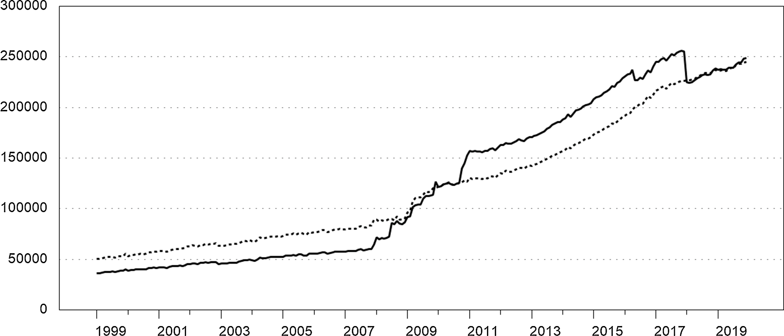
Figure 1. Noninterest-bearing monetary assets. Monthly. The solid series is the amount outstanding. The break-adjusted series is dotted.
2.2. User Costs of Components
Real user costs of the monetary assets are based on the following formula:
 \begin{equation}\pi _{it}=\frac{R_{t}-r_{i,t}}{1+R_{t}}\end{equation}
where $R_{t}$
denotes a benchmark rate of return and
$R_{t}$
denotes a benchmark rate of return and $r_{i,t}$
is the own rate of return on the
$r_{i,t}$
is the own rate of return on the $i$
th monetary asset; see Barnett (Reference Barnett1978) and Donovan (Reference Donovan1978). Hancock (Reference Hancock2005) outlined a series of major revisions to the construction of the Bank of England’s Divisia aggregates including introducing an envelope approach to measure the benchmark rate. With this approach, the benchmark rate is the highest rate of return among the set of monetary assets. As explained by Hancock (Reference Hancock2005), the benchmark rate for the household-sector was the rate on Tax Exempt Special Savings Accounts (TESSAs) beginning in 1991 and then the rate of return on Individual Savings Accounts (ISAs) beginning in 1999. Hancock (Reference Hancock2005, p. 41) argued this was appropriate since “because of their tax treatment these accounts are largely held to satisfy a savings motive.”Footnote
4
Berar and Olwadi (Reference Berar and Olwadi2013) observe, however, that “[t]he benchmark rate for household Divisia money has tended to be the rate on time deposits excluding ISAs” rather than the ISA rate. In the Bank of England’s Divisia measure, when the interest rate on ISAs falls below the upper envelope, ISAs have a positive expenditure share, whereas the monetary asset associated with the highest rate will have an expenditure share of zero. We do not include ISAs as a component in our demand system following Hancock’s reasoning.
$i$
th monetary asset; see Barnett (Reference Barnett1978) and Donovan (Reference Donovan1978). Hancock (Reference Hancock2005) outlined a series of major revisions to the construction of the Bank of England’s Divisia aggregates including introducing an envelope approach to measure the benchmark rate. With this approach, the benchmark rate is the highest rate of return among the set of monetary assets. As explained by Hancock (Reference Hancock2005), the benchmark rate for the household-sector was the rate on Tax Exempt Special Savings Accounts (TESSAs) beginning in 1991 and then the rate of return on Individual Savings Accounts (ISAs) beginning in 1999. Hancock (Reference Hancock2005, p. 41) argued this was appropriate since “because of their tax treatment these accounts are largely held to satisfy a savings motive.”Footnote
4
Berar and Olwadi (Reference Berar and Olwadi2013) observe, however, that “[t]he benchmark rate for household Divisia money has tended to be the rate on time deposits excluding ISAs” rather than the ISA rate. In the Bank of England’s Divisia measure, when the interest rate on ISAs falls below the upper envelope, ISAs have a positive expenditure share, whereas the monetary asset associated with the highest rate will have an expenditure share of zero. We do not include ISAs as a component in our demand system following Hancock’s reasoning.
Berar and Olwadi (Reference Berar and Olwadi2013) explain that a new effective rate of return on ISAs was introduced in January 2011. They predicted that the new effective rate series for ISAs would “most likely” be the benchmark rate in the future. They show that the new ISA rate is considerably higher than the old one and that the change led to significant revisions to household-sector Divisia money growth. Berar and Olwadi (Reference Berar and Olwadi2013) further explain that the interest rate on time deposits excluding ISAs used to calculate the household-sector Divisia measure is also affected by the change, since that rate is “calculated by residual based on the interest rates for all time deposits and the interest rates for ISAs.” We adopt an alternative approach to construct user costs for our empirical analysis. The Bank of England publishes an extensive set of monthly effective interest rate series based on a representative sample of MFIs covering 75% of business in each sector, although only banks are included before 2010. According to the Bank of England, “from January 2010, the published data are combined bank and building society rates for all series instead of a bank-only rate.”Footnote 5 We use the household-sector rates on outstanding sterling deposits with UK MFIs for sight deposits and time deposits from this source as own rates for the corresponding components.
For NIBM, the own rate ( $r_{i,t}$
) is zero and, consequently, their user cost varies directly with the benchmark rate,
$r_{i,t}$
) is zero and, consequently, their user cost varies directly with the benchmark rate, $R_{t}$
. For interest-bearing sight and time deposits,
$R_{t}$
. For interest-bearing sight and time deposits, $r_{i,t}$
is measured by the effective rates as described above. These own rates are shown in Figure 2. The recession from 2008Q2 to 2009Q2 is shaded.Footnote
6
We set the benchmark rate equal to the upper envelope of the two deposit rates plus a small liquidity premium, which ensures positive user costs and expenditure shares for both components. In practice, the time deposit rate exceeds the sight deposit rate throughout our sample, so our approach implies that the user cost for sight deposits varies with the spread between the time deposit rate and the sight deposit rate.
$r_{i,t}$
is measured by the effective rates as described above. These own rates are shown in Figure 2. The recession from 2008Q2 to 2009Q2 is shaded.Footnote
6
We set the benchmark rate equal to the upper envelope of the two deposit rates plus a small liquidity premium, which ensures positive user costs and expenditure shares for both components. In practice, the time deposit rate exceeds the sight deposit rate throughout our sample, so our approach implies that the user cost for sight deposits varies with the spread between the time deposit rate and the sight deposit rate.
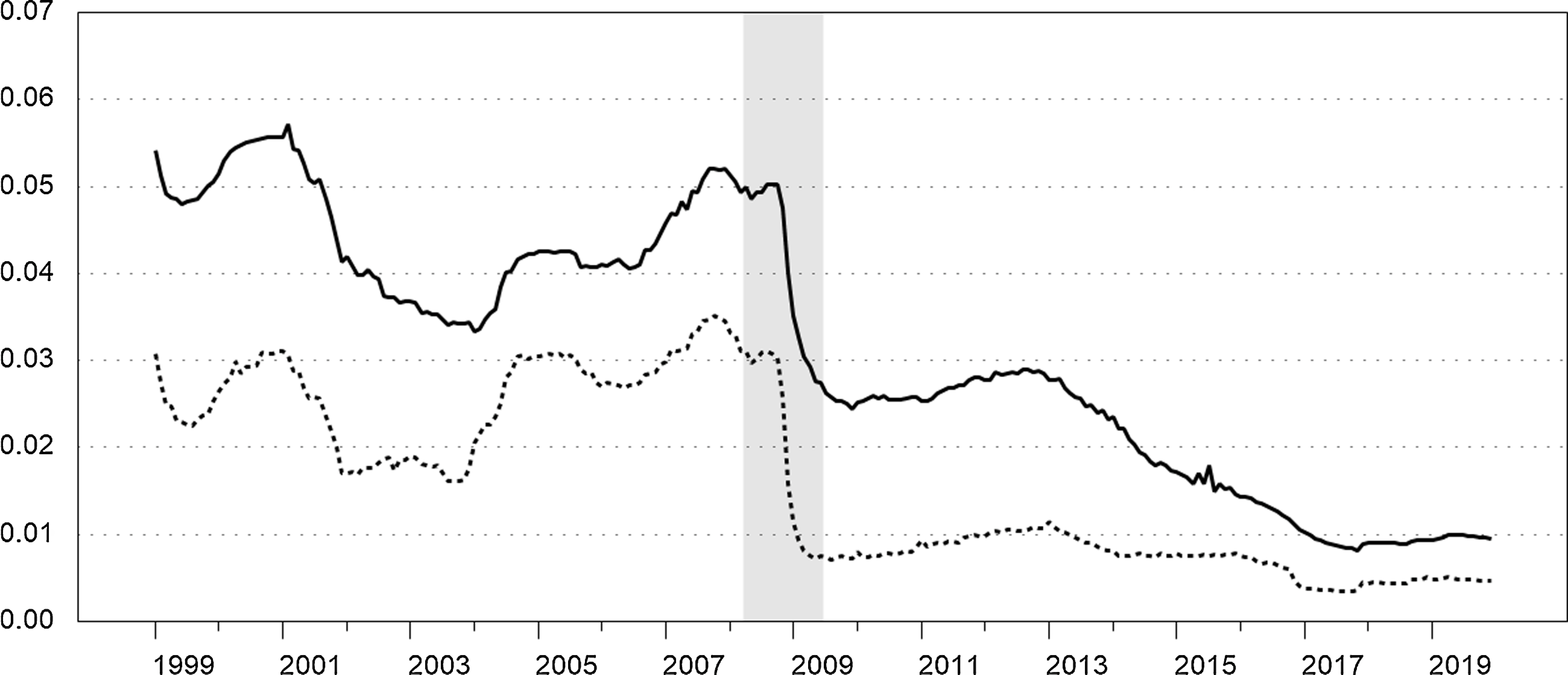
Figure 2. Household-sector own rates. Monthly. Effective interest rates, UK MFIs, outstanding deposits. The solid series is the interest rate on time deposits and the dotted series is the rate on interest-bearing sight deposits. Recession is shaded.
Incorporating a liquidity premium in the benchmark rate is common in the Divisia literature. Bissoondeeal et al. (Reference Bissoondeeal, Jones, Binner and Mullineux2010) used a benchmark rate equal to the 3-month Treasury bill rate plus 250 basis points in their UK study covering 1977–2008.Footnote 7 Stracca (Reference Stracca2004) constructed a Euro-11 Divisia M3 aggregate for 1980–2000. He set the benchmark rate equal to a 3-month market interest rate, which exceeded the estimated own rates of the other components, plus a liquidity premium of 60 basis points. He states (p. 317) “that similar values of the premium lead to very similar patterns of the Divisia monetary aggregate.” Anderson and Jones (Reference Anderson and Jones2011) calculated Divisia aggregates for the USA using their “preferred” benchmark rate equal to the upper envelope of the own rates of return for their broadest Divisia index for the USA as well as a set of short-term market rates plus 100 basis points.Footnote 8 We chose to use the more conservative value of 60 basis points for our liquidity premium.
3. Fourier demand system
We estimate elasticities of substitution from the semi-nonparametric Fourier flexible functional form because it is dense in a Sobolev norm and can globally approximate the levels and partial derivatives of a continuous utility function giving arbitrary unconstrained estimates of elasticities of substitution; see Gallant (Reference Gallant1981) and El Badawi et al. (Reference El Badawi, Gallant and Souza1983). The asymptotically ideal model (AIM) of Barnett and Jonas (Reference Barnett and Jonas1983) is an alternative functional form with the same property. For the UK, Drake et al. (Reference Drake, Fleissig and Swofford2003) estimated an AIM model for components of the Bank of England’s personal-sector Divisia aggregate from 1977 to 1994.Footnote 9 Drake and Fleissig (Reference Drake and Fleissig2004) estimated a Fourier demand model for UK monetary assets that includes foreign currency holdings of sterling from several European countries.Footnote 10 A main advantage of the AIM and Fourier demand models is that they can provide global approximations to the underlying data generating function.Footnote 11
Let $\boldsymbol{a}_{t}$
be the vector of real, per capita, quantities of the three components in period
$\boldsymbol{a}_{t}$
be the vector of real, per capita, quantities of the three components in period $t$
and let
$t$
and let $\boldsymbol{\gamma }_{t}$
be the corresponding vector of nominal user costs. Nominal user costs are equal to real user costs multiplied by an appropriate price index. The three household-sector monetary assets are as follows:
$\boldsymbol{\gamma }_{t}$
be the corresponding vector of nominal user costs. Nominal user costs are equal to real user costs multiplied by an appropriate price index. The three household-sector monetary assets are as follows: $a_{1}$
denotes NIBM,
$a_{1}$
denotes NIBM, $a_{2}$
denotes interest-bearing MFI sight deposits, and
$a_{2}$
denotes interest-bearing MFI sight deposits, and $a_{3}$
denotes MFI time deposits. Expenditure shares for the three components are given by
$a_{3}$
denotes MFI time deposits. Expenditure shares for the three components are given by $s_{i,t}=\gamma _{i,t}a_{i,t}/y_{t}$
, and
$s_{i,t}=\gamma _{i,t}a_{i,t}/y_{t}$
, and $\boldsymbol{v}_{t}=\boldsymbol{\gamma }_{t}/y_{t}$
is the vector of expenditure normalized user costs, where
$\boldsymbol{v}_{t}=\boldsymbol{\gamma }_{t}/y_{t}$
is the vector of expenditure normalized user costs, where $y_{t}=\boldsymbol{\gamma }_{t}'\boldsymbol{a}_{t}$
is total expenditure on monetary services. As in Serletis and Xu (Reference Serletis and Xu2020), weak separability is a maintained hypothesis in our model; see Jin (Reference Jin2016), Barnett and Gaekwad (Reference Barnett and Gaekwad2018), Chang and Serletis (Reference Chang and Serletis2019), and Fleissig and Swofford (Reference Fleissig and Swofford2020) for additional discussion.Footnote
12
We assume that the three household-sector monetary assets are a weakly separable block, which implies that the marginal rates of substitution between these assets are independent of the quantities of all other decisions variables such as consumption and leisure. Consequently, the second-stage utility maximization problem can be written as
$y_{t}=\boldsymbol{\gamma }_{t}'\boldsymbol{a}_{t}$
is total expenditure on monetary services. As in Serletis and Xu (Reference Serletis and Xu2020), weak separability is a maintained hypothesis in our model; see Jin (Reference Jin2016), Barnett and Gaekwad (Reference Barnett and Gaekwad2018), Chang and Serletis (Reference Chang and Serletis2019), and Fleissig and Swofford (Reference Fleissig and Swofford2020) for additional discussion.Footnote
12
We assume that the three household-sector monetary assets are a weakly separable block, which implies that the marginal rates of substitution between these assets are independent of the quantities of all other decisions variables such as consumption and leisure. Consequently, the second-stage utility maximization problem can be written as $\max _{\boldsymbol{a}}U(\boldsymbol{a})$
, subject to a budget constraint of the form
$\max _{\boldsymbol{a}}U(\boldsymbol{a})$
, subject to a budget constraint of the form $\boldsymbol{\gamma }'\boldsymbol{a}=y$
; see, for example, Barnett and Gaekwad (Reference Barnett and Gaekwad2018, p. 260).
$\boldsymbol{\gamma }'\boldsymbol{a}=y$
; see, for example, Barnett and Gaekwad (Reference Barnett and Gaekwad2018, p. 260).
We form quarterly averages of the monthly break-adjusted components and convert them to real terms using an implicit price index for total UK domestic consumption. The quarterly averaged real user cost series are converted to nominal terms using the same price index. Real quantities are converted to per-capita terms using the quarterly interpolated mid-year UK resident population. The price index is the ratio of total UK domestic household final consumption expenditure at current prices (seasonally adjusted) to the corresponding chained volume measure from Consumer Trends (Office for National Statistics). The quarterly interpolated population series is also from the Office for National Statistics. The estimation period for the Fourier demand system is 1999Q1 to 2019Q4.
The Fourier flexible form indirect utility function is defined as follows (Gallant, Reference Gallant1981):
 \begin{equation}f\left(\boldsymbol{v},\boldsymbol{\theta }\right)=u_{0}+\boldsymbol{b}'\boldsymbol{v}+\frac{1}{2}\boldsymbol{v}\boldsymbol{'}\boldsymbol{Cv}+\sum _{\alpha =1}^{A}\left(u_{0\alpha }+2\sum _{j=1}^{J}\left[u_{j\alpha }\cos \left(j\boldsymbol{k}_{\alpha }^{'}\boldsymbol{v}\right)-w_{j\alpha }\sin \left(j\boldsymbol{k}_{\alpha }^{'}\boldsymbol{v}\right)\right]\right)\end{equation}
where $C=-\sum _{\alpha =1}^{A}u_{0\alpha }\boldsymbol{k}_{\alpha }\boldsymbol{k}_{\alpha }^{'}$
and the vector of parameters to be estimated
$C=-\sum _{\alpha =1}^{A}u_{0\alpha }\boldsymbol{k}_{\alpha }\boldsymbol{k}_{\alpha }^{'}$
and the vector of parameters to be estimated $\theta =\{\boldsymbol{b},u_{0\alpha },u_{j\alpha },w_{j\alpha }\colon j=1,2,\ldots,J; \alpha =1,2,\ldots,A\}$
. A multi-index,
k
α
, denotes partial differentiation of the utility function. The corresponding share equations
$\theta =\{\boldsymbol{b},u_{0\alpha },u_{j\alpha },w_{j\alpha }\colon j=1,2,\ldots,J; \alpha =1,2,\ldots,A\}$
. A multi-index,
k
α
, denotes partial differentiation of the utility function. The corresponding share equations
 \begin{equation}s_{i}\left(\boldsymbol{v},\boldsymbol{\theta }\right)=\frac{b_{i}v_{i}-\sum _{\alpha =1}^{A}\left(u_{0\alpha }\boldsymbol{v}'\boldsymbol{k}_{\alpha }+2\sum _{j=1}^{J}j\left[u_{j\alpha }\sin \left(j\boldsymbol{k}_{\alpha }^{'}\boldsymbol{v}\right)+w_{j\alpha }\cos \left(j\boldsymbol{k}_{\alpha }^{'}\boldsymbol{v}\right)\right]\right)k_{i\alpha }v_{i}}{\boldsymbol{b}'\boldsymbol{v}-\sum _{\alpha =1}^{A}\left(u_{0\alpha }\boldsymbol{v}'\boldsymbol{k}_{\alpha }+2\sum _{j=1}^{J}j\left[u_{j\alpha }\sin \left(j\boldsymbol{k}_{\alpha }^{'}\boldsymbol{v}\right)+w_{j\alpha }\cos \left(j\boldsymbol{k}_{\alpha }^{'}\boldsymbol{v}\right)\right]\right)\boldsymbol{k}_{\alpha }^{'}\boldsymbol{v}}\end{equation}
are estimated using the International TSP 4.5 seemingly unrelated regression procedure. Following Gallant (Reference Gallant1981), we scale the expenditure normalized user costs so that $0\lt v_{i}\lt 2\pi$
. The parameters of the Fourier demand system are homogenous of degree zero, and the normalization of
$0\lt v_{i}\lt 2\pi$
. The parameters of the Fourier demand system are homogenous of degree zero, and the normalization of $b_{3}=-1$
is imposed to estimate the system of share equations. The number of terms and degree of the Fourier polynomials are determined by the parameters
$b_{3}=-1$
is imposed to estimate the system of share equations. The number of terms and degree of the Fourier polynomials are determined by the parameters $A$
and
$A$
and $J$
through empirical testing. The degree of the Fourier polynomials are determined by the upward F-test procedure of Eastwood (Reference Eastwood1991), and multiple multi-indices with multiple starting values were used to ensure convergence to the global optimum as in Drake and Fleissig (Reference Drake and Fleissig2004, Reference Drake and Fleissig2008, Reference Drake and Fleissig2009, Reference Drake and Fleissig2010), Jones et al. (Reference Jones, Fleissig, Elger and Dutkowsky2008), Anderson et al. (Reference Anderson, Duca, Fleissig and Jones2019), and Fleissig and Swofford (Reference Fleissig and Swofford2020). There was evidence of autocorrelation in the demand system. A first-order vector autoregressive process is applied to correct for serial correlation (Berndt and Savin, Reference Berndt and Savin1975). Convergence was set at 0.00001 with estimates of
$J$
through empirical testing. The degree of the Fourier polynomials are determined by the upward F-test procedure of Eastwood (Reference Eastwood1991), and multiple multi-indices with multiple starting values were used to ensure convergence to the global optimum as in Drake and Fleissig (Reference Drake and Fleissig2004, Reference Drake and Fleissig2008, Reference Drake and Fleissig2009, Reference Drake and Fleissig2010), Jones et al. (Reference Jones, Fleissig, Elger and Dutkowsky2008), Anderson et al. (Reference Anderson, Duca, Fleissig and Jones2019), and Fleissig and Swofford (Reference Fleissig and Swofford2020). There was evidence of autocorrelation in the demand system. A first-order vector autoregressive process is applied to correct for serial correlation (Berndt and Savin, Reference Berndt and Savin1975). Convergence was set at 0.00001 with estimates of $A=3$
and
$A=3$
and $J=1$
determined by the upward F test procedure of Eastwood (Reference Eastwood1991). The Fourier parameter estimates are provided in Table 1. The share equations provide an accurate approximation to the data in terms of the R-square and root mean square error. The Q-statistic with the Box−Pierce test for autocorrelation for each share indicate white noise at the five percent level.
$J=1$
determined by the upward F test procedure of Eastwood (Reference Eastwood1991). The Fourier parameter estimates are provided in Table 1. The share equations provide an accurate approximation to the data in terms of the R-square and root mean square error. The Q-statistic with the Box−Pierce test for autocorrelation for each share indicate white noise at the five percent level.
Theoretical regularity conditions for positivity, monotonicity, and curvature for the Fourier flexible form demand system have been evaluated by Serletis and Shahmoradi (Reference Serletis and Shahmoradi2005) and Drake and Fleissig (Reference Drake and Fleissig2009), and we follow their procedures.Footnote
13
Positivity is satisfied if the estimated share equations are nonnegative ( $s_{i}(\boldsymbol{v},\hat{\boldsymbol{\theta }})\geq 0$
) for all assets. Monotonicity is satisfied if the gradient of the estimated indirect utility function is strictly negative (
$s_{i}(\boldsymbol{v},\hat{\boldsymbol{\theta }})\geq 0$
) for all assets. Monotonicity is satisfied if the gradient of the estimated indirect utility function is strictly negative ( $\nabla f(\boldsymbol{v},\hat{\boldsymbol{\theta }})\lt 0$
), and curvature is satisfied if the Slutsky matrix is negative semi-definite.Footnote
14
For this UK dataset, there were no violations of regularity conditions. Serletis and Shahmoradi (Reference Serletis and Shahmoradi2005) and Drake and Fleissig (Reference Drake and Fleissig2009) found some curvature violations when estimating the Fourier flexible form. These papers also provide estimates of the model with curvature conditions imposed following the approach of Gallant and Golub (Reference Gallant and Golub1984).Footnote
15
$\nabla f(\boldsymbol{v},\hat{\boldsymbol{\theta }})\lt 0$
), and curvature is satisfied if the Slutsky matrix is negative semi-definite.Footnote
14
For this UK dataset, there were no violations of regularity conditions. Serletis and Shahmoradi (Reference Serletis and Shahmoradi2005) and Drake and Fleissig (Reference Drake and Fleissig2009) found some curvature violations when estimating the Fourier flexible form. These papers also provide estimates of the model with curvature conditions imposed following the approach of Gallant and Golub (Reference Gallant and Golub1984).Footnote
15
4. Elasticities of substitution
We estimate Morishma elasticities of substitution from the Fourier demand model. Let $ME_{ij}$
denote the Morishima elasticity of substitution between monetary asset
$ME_{ij}$
denote the Morishima elasticity of substitution between monetary asset $i$
and monetary asset
$i$
and monetary asset $j$
, which characterizes substitution between these assets in response to a ceteris paribus change in the user cost of asset
$j$
, which characterizes substitution between these assets in response to a ceteris paribus change in the user cost of asset $i$
(
$i$
( $\gamma _{i}$
).Footnote
16
The Morishima elasticity shows how agents substitute funds between the pairs of assets in response to a change in one of the asset’s user costs and determines whether substitution is elastic or inelastic in response to such a change. More technically, Blackorby and Russell (Reference Blackorby and Russell1989) show that
$\gamma _{i}$
).Footnote
16
The Morishima elasticity shows how agents substitute funds between the pairs of assets in response to a change in one of the asset’s user costs and determines whether substitution is elastic or inelastic in response to such a change. More technically, Blackorby and Russell (Reference Blackorby and Russell1989) show that $\frac{\partial ln(\gamma _{i}x_{i}^{*}/\gamma _{j}x_{j}^{*})}{\partial ln(\gamma _{i}/\gamma _{j})}=1-ME_{ij}$
, where
$\frac{\partial ln(\gamma _{i}x_{i}^{*}/\gamma _{j}x_{j}^{*})}{\partial ln(\gamma _{i}/\gamma _{j})}=1-ME_{ij}$
, where $x_{i}^{*}$
denotes the compensated demand for asset
$x_{i}^{*}$
denotes the compensated demand for asset $i$
. Monetary assets are elastic (inelastic) substitutes when
$i$
. Monetary assets are elastic (inelastic) substitutes when $ME_{ij}\gt 1$
(
$ME_{ij}\gt 1$
( $0\lt ME_{ij}\lt 1$
). Thus, inelastic substitution implies that, holding utility constant, the share of asset
$0\lt ME_{ij}\lt 1$
). Thus, inelastic substitution implies that, holding utility constant, the share of asset $i$
decreases relative to the share of asset
$i$
decreases relative to the share of asset $j$
when the user cost of the ith asset decreases. The Morishima elasticity need not be symmetric, because
$j$
when the user cost of the ith asset decreases. The Morishima elasticity need not be symmetric, because $ME_{ij}$
captures substitution in response to a ceteris paribus change in
$ME_{ij}$
captures substitution in response to a ceteris paribus change in $\gamma _{i}$
, whereas
$\gamma _{i}$
, whereas $ME_{ji}$
relates to a ceteris paribus change in
$ME_{ji}$
relates to a ceteris paribus change in $\gamma _{j}$
.
$\gamma _{j}$
.
Table 1. Parameters of Fourier flexible form
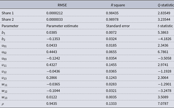
Note: The estimation is performed in International TSP 4.5 with convergence set at 0.00001. Multiple starting values and multi-indexes were used to ensure convergence to the global optimum. The upward F-test procedure of Eastwood (Reference Eastwood1991) is used to determine the degree of the of the Fourier polynomials with $A=3$
and
$A=3$
and $J=1$
, and a normalization of
$J=1$
, and a normalization of $b_{3}=-1$
is imposed in estimation. A first-order vector autoregressive process as in Berndt and Savin (Reference Berndt and Savin1975) was used to correct for serial correlation.
$b_{3}=-1$
is imposed in estimation. A first-order vector autoregressive process as in Berndt and Savin (Reference Berndt and Savin1975) was used to correct for serial correlation.
Figure 3 shows the quarterly real user costs for NIBM and interest-bearing MFI sight deposits. We do not show the user cost for MFI time deposits in the figure, since in practice the benchmark rate is the time deposit rate plus the liquidity premium. The user cost of NIBM follows the benchmark rate since its own rate is zero. Consequently, the user cost of NIBM declines significantly during 2001–2003 and again during the 2008–2009 recession. The user cost of MFI sight deposits is roughly constant during 1999–2001, then declines through mid-2004, but then gradually trends upward until the 2008–2009 recession. During the recession, the user cost increases initially, but then decreases and is then roughly constant through the end of 2012. Both user costs gradually decline in tandem beginning around 2013.
Morishima elasticities are calculated at each observation from the estimated Fourier demand system and are all significantly different from zero at the 5% level. As Barnett et al. (Reference Barnett, Fisher and Serletis1992) explain, estimated elasticities of substitution change over the sample corresponding to changes in the underlying user cost data used to estimate the demand system model from which the estimated substitution elasticities are derived. Table 2 presents the minimum and maximum values of these estimated elasticities over the sample as well the sample average and standard deviation. The summary statistics provide strong evidence of asymmetry with respect to $ME_{12}$
and
$ME_{12}$
and $ME_{21}$
. These elasticities relate to substitution between NIBM (
$ME_{21}$
. These elasticities relate to substitution between NIBM ( $a_{1}$
) and interest-bearing MFI sight deposits (
$a_{1}$
) and interest-bearing MFI sight deposits ( $a_{2}$
) in response to ceteris paribus changes in the user costs of NIBM and sight deposits, respectively.
$a_{2}$
) in response to ceteris paribus changes in the user costs of NIBM and sight deposits, respectively. $ME_{12}$
is 0.866 on average with a maximum value of 0.95 implying inelastic substitution throughout the sample between NIBM and sight deposits in response to a change in the user cost of NIBM. In contrast, the minimum value of
$ME_{12}$
is 0.866 on average with a maximum value of 0.95 implying inelastic substitution throughout the sample between NIBM and sight deposits in response to a change in the user cost of NIBM. In contrast, the minimum value of $ME_{21}$
is 1.548 indicating that substitution between these assets is elastic in response to a change in the user cost of sight deposits throughout the sample.
$ME_{21}$
is 1.548 indicating that substitution between these assets is elastic in response to a change in the user cost of sight deposits throughout the sample.
Table 2. Morishima elasticities of substitution
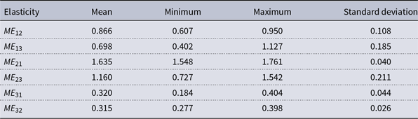
Note: $ME_{ij}$
= Morishima elasticity of substitution between assets
$ME_{ij}$
= Morishima elasticity of substitution between assets $i$
and
$i$
and $j$
for a change in the user cost of asset
$j$
for a change in the user cost of asset $i$
.
$i$
. $a_{1}$
denotes noninterest-bearing monetary assets (NIBM).
$a_{1}$
denotes noninterest-bearing monetary assets (NIBM). $a_{2}$
denotes interest-bearing MFI sight deposits.
$a_{2}$
denotes interest-bearing MFI sight deposits. $a_{3}$
denotes MFI time deposits.
$a_{3}$
denotes MFI time deposits.
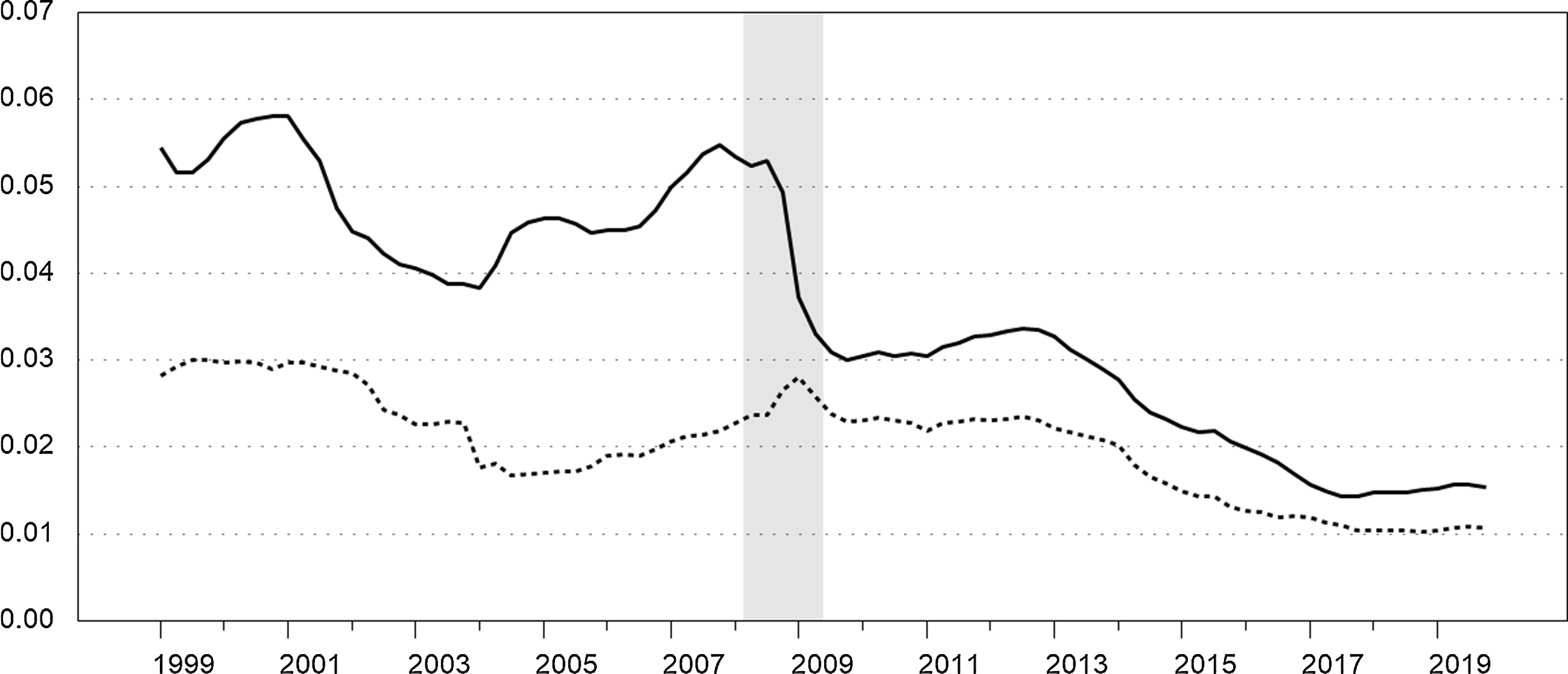
Figure 3. Real user costs. Quarterly. The solid series is the user cost of noninterest-bearing monetary assets (NIBM). The dotted series is the user cost of sight deposits. Recession is shaded.
The summary statistics also provide strong evidence of asymmetry with respect to $ME_{23}$
and
$ME_{23}$
and $ME_{32}$
, which relate to substitution between interest-bearing MFI sight deposits (
$ME_{32}$
, which relate to substitution between interest-bearing MFI sight deposits ( $a_{2}$
) and MFI time deposits (
$a_{2}$
) and MFI time deposits ( $a_{3}$
) in response to ceteris paribus changes in the user costs of sight and time deposits, respectively. The average value of
$a_{3}$
) in response to ceteris paribus changes in the user costs of sight and time deposits, respectively. The average value of $ME_{32}$
is 0.315 as compared to an average value of 1.16 for
$ME_{32}$
is 0.315 as compared to an average value of 1.16 for $ME_{23}$
and
$ME_{23}$
and $ME_{32}$
is less than 0.4 throughout the sample, whereas
$ME_{32}$
is less than 0.4 throughout the sample, whereas $ME_{23}$
is always above 0.7. We also find that
$ME_{23}$
is always above 0.7. We also find that $ME_{13}$
exceeds
$ME_{13}$
exceeds $ME_{31}$
throughout our sample, although their ranges overlap slightly. Thus, all three pairs of Morishima elasticities exhibit asymmetry throughout our sample.
$ME_{31}$
throughout our sample, although their ranges overlap slightly. Thus, all three pairs of Morishima elasticities exhibit asymmetry throughout our sample.
Figure 4 shows the Morishima elasticities of substitution between NIBM and sight deposits, $ME_{12}$
and
$ME_{12}$
and $ME_{21}$
, over our sample. As the figure shows,
$ME_{21}$
, over our sample. As the figure shows, $ME_{12}$
is roughly constant and just below unity throughout most of the sample, but then declines significantly in the last several years.
$ME_{12}$
is roughly constant and just below unity throughout most of the sample, but then declines significantly in the last several years. $ME_{21}$
lies within a narrow band and is above 1.5 throughout the sample. Figure 5 shows the Morishima elasticities between sight and time deposits,
$ME_{21}$
lies within a narrow band and is above 1.5 throughout the sample. Figure 5 shows the Morishima elasticities between sight and time deposits, $ME_{23}$
and
$ME_{23}$
and $ME_{32}$
.
$ME_{32}$
. $ME_{23}$
is almost always above unity until mid-2014, implying elastic substitution, but it declines in the latter part of our sample and is below unity from the last quarter of 2014 through the end of the sample. As previously noted,
$ME_{23}$
is almost always above unity until mid-2014, implying elastic substitution, but it declines in the latter part of our sample and is below unity from the last quarter of 2014 through the end of the sample. As previously noted, $ME_{32}$
is always below 0.4 throughout the sample.
$ME_{32}$
is always below 0.4 throughout the sample.
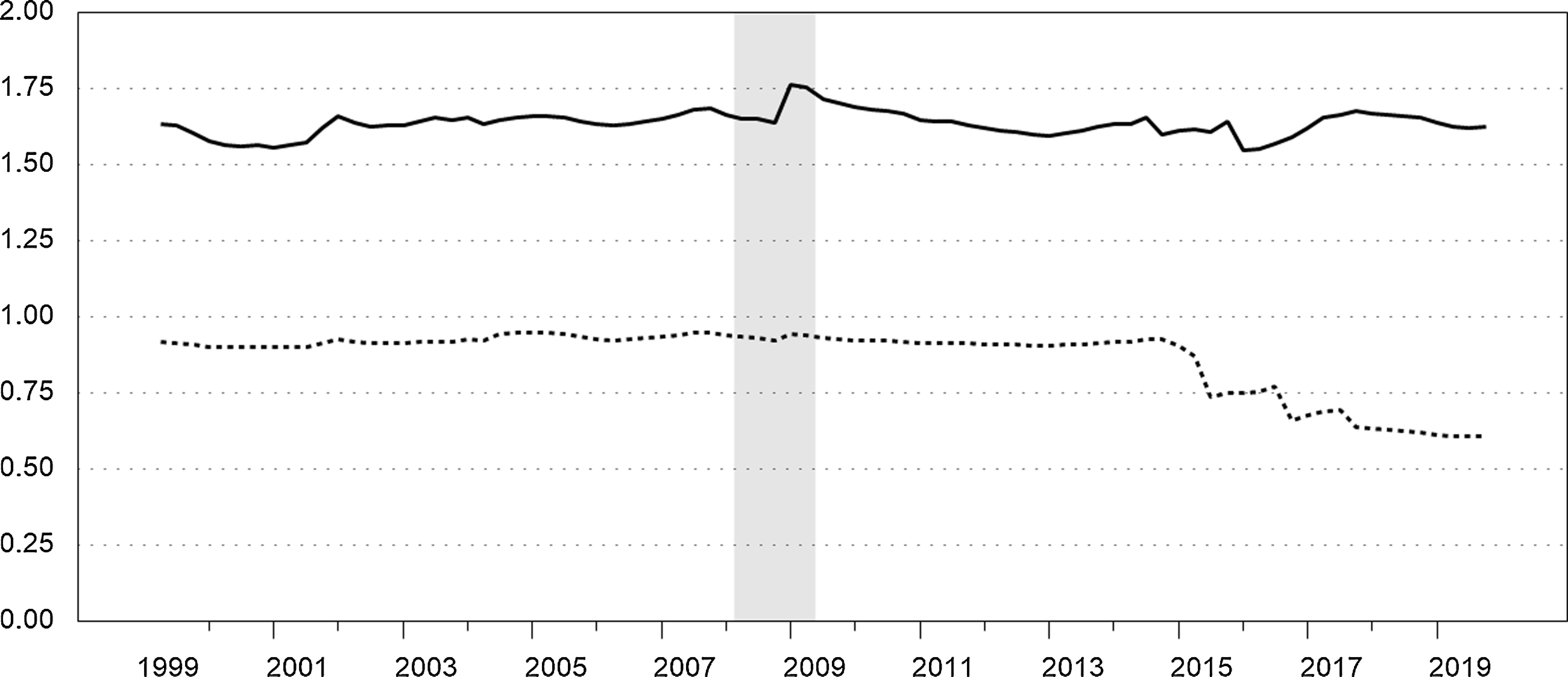
Figure 4. Morishima elasticities of substitution between NIBM and interest-bearing MFI sight deposits. Quarterly. The solid series is $ME_{21}$
. The dotted series is
$ME_{21}$
. The dotted series is $ME_{12}$
. Recession is shaded.
$ME_{12}$
. Recession is shaded.
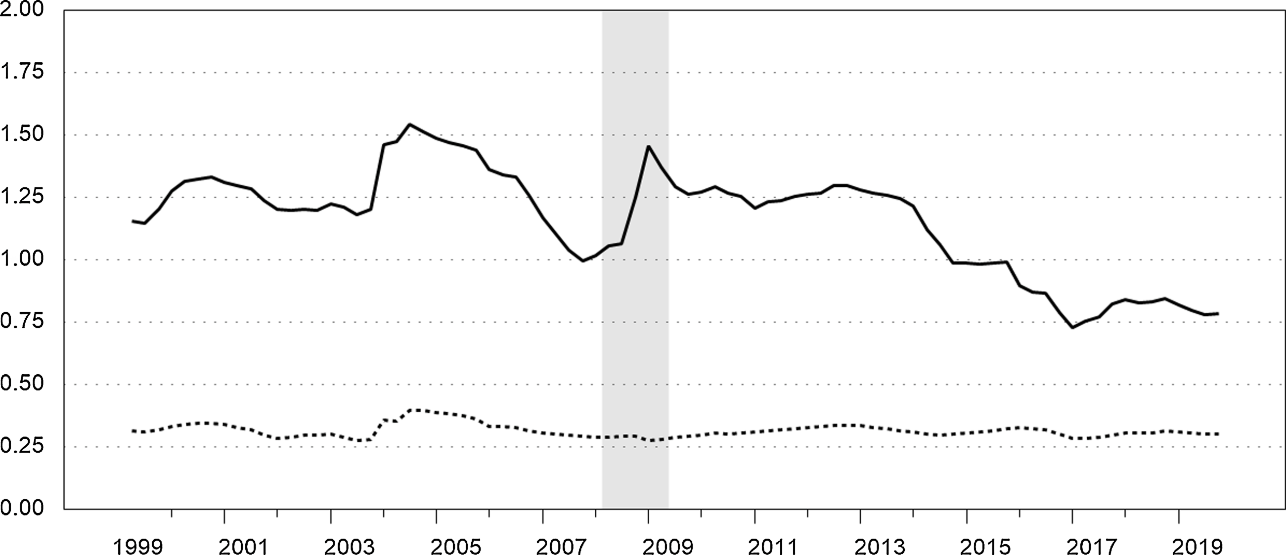
Figure 5. Morishima elasticities of substitution between sight and time deposits. Quarterly. The solid series is $ME_{23}$
. The dotted series is
$ME_{23}$
. The dotted series is $ME_{32}$
. Recession is shaded.
$ME_{32}$
. Recession is shaded.
Asymmetric Morishima elasticities of substitution between monetary assets are a common finding in the literature (see, e.g., Fleissig and Swofford, Reference Fleissig and Swofford2020), and our findings have some precedent in the previous UK literature. Drake et al. (Reference Drake, Fleissig and Swofford2003) estimate Morishima elasticities for UK personal-sector monetary assets from 1977 to 1994 for three components: NIBM, an aggregate of interest-bearing sight deposits and building society deposits, and time deposits at banks.Footnote
17
They find “the strongest and most consistent evidence of asset substitution” between their aggregate of interest-bearing sight deposits and building society deposits and time deposits at banks (p. 112). The corresponding elasticities from their study are roughly comparable to our $ME_{23}$
and
$ME_{23}$
and $ME_{32}$
, which are based on MFI sight and time deposits. They find that
$ME_{32}$
, which are based on MFI sight and time deposits. They find that $ME_{32}$
is below
$ME_{32}$
is below $ME_{23}$
throughout their sample with estimates of
$ME_{23}$
throughout their sample with estimates of $ME_{32}$
that are well below unity and sometimes negative (indicating complementarity). Notably, given the differences in time periods and the definitions of the components, their estimate of
$ME_{32}$
that are well below unity and sometimes negative (indicating complementarity). Notably, given the differences in time periods and the definitions of the components, their estimate of $ME_{23}$
at the end of 1994 and our estimate of the roughly comparable elasticity based on MFI sight and time deposits at the beginning of our sample are very close. Drake et al. (Reference Drake, Fleissig and Swofford2003) also estimate Morishima elasticities between NIBM and their aggregate of interest-bearing sight deposits and building society deposits, which are roughly comparable to our
$ME_{23}$
at the end of 1994 and our estimate of the roughly comparable elasticity based on MFI sight and time deposits at the beginning of our sample are very close. Drake et al. (Reference Drake, Fleissig and Swofford2003) also estimate Morishima elasticities between NIBM and their aggregate of interest-bearing sight deposits and building society deposits, which are roughly comparable to our $ME_{12}$
and
$ME_{12}$
and $ME_{21}$
. Their estimates of
$ME_{21}$
. Their estimates of $ME_{21}$
are usually higher than their estimates of
$ME_{21}$
are usually higher than their estimates of $ME_{12}$
, and their estimate of
$ME_{12}$
, and their estimate of $ME_{21}$
at the end of 1994 is also very close to our estimate of the roughly comparable elasticity at the beginning of our sample. On the other hand, Drake, Fleissig, and Swofford’s estimates of
$ME_{21}$
at the end of 1994 is also very close to our estimate of the roughly comparable elasticity at the beginning of our sample. On the other hand, Drake, Fleissig, and Swofford’s estimates of $ME_{12}$
are frequently very low and sometimes negative, and their estimates of
$ME_{12}$
are frequently very low and sometimes negative, and their estimates of $ME_{13}$
are frequently negative and are often below their estimates of
$ME_{13}$
are frequently negative and are often below their estimates of $ME_{31}$
.
$ME_{31}$
.
Jones et al. (Reference Jones, Fleissig, Elger and Dutkowsky2008) estimate a Fourier demand model for the USA and argue that a particular subset of the Morishima elasticities can be used to “directly characterize monetary asset substitution responses to monetary policy.” Their benchmark rate was based on the 6-month Treasury bill rate, which was highly correlated with the Federal Funds rate. As a result, the user cost of noninterest-bearing monetary assets moved in line with the Federal Funds rate. In contrast, the own rates on small-time deposits and money market funds “move closely in line with Treasury bill rates” implying that their user costs “should be largely invariant to Federal Funds rate changes.” Consequently, Jones et al. (Reference Jones, Fleissig, Elger and Dutkowsky2008) characterize monetary asset substitution in response to changes in the Federal Funds rate in terms of Morishima elasticities between noninterest-bearing assets and both small-time deposits and money market funds in response to changes in the user cost of noninterest-bearing assets and similarly for checkable deposits and savings deposits; see also Fleissig and Jones (Reference Fleissig and Jones2015).
For our household-sector UK model, the Morishima elasticities that are most relevant to monetary policy are $ME_{12}$
and
$ME_{12}$
and $ME_{13}$
, which measures substitution between NIBM and sight and time deposits, respectively, in response to changes in the user cost of NIBM. Prior to the 2008–2009 recession, changes in the Bank of England’s official Bank Rate are reflected in the own rate of return on time deposits and, consequently, in the user cost of NIBM, since the benchmark rate is the time deposit rate plus a small liquidity premium. Bank Rate was reduced to 2% by the end of 2008 and to 0.5% in March of 2009. The own rates of return on both sight and time deposits declined heading into the 2008–2009 recession and declined sharply during the recession as seen in Figure 2. The user cost of NIBM declined heading into the 2008–2009 recession and then declined sharply during the recession before stabilizing. In contrast, the user cost of MFI sight deposits was gradually trending upward heading into the recession. During the recession, it increased initially but then decreased. As seen in Figure 3, if we compare their values at the end of 2009 to those at the beginning of 2008, thus encompassing the recession, the user cost of NIBM decreased significantly, while the user cost of sight deposits was roughly constant. Consequently,
$ME_{13}$
, which measures substitution between NIBM and sight and time deposits, respectively, in response to changes in the user cost of NIBM. Prior to the 2008–2009 recession, changes in the Bank of England’s official Bank Rate are reflected in the own rate of return on time deposits and, consequently, in the user cost of NIBM, since the benchmark rate is the time deposit rate plus a small liquidity premium. Bank Rate was reduced to 2% by the end of 2008 and to 0.5% in March of 2009. The own rates of return on both sight and time deposits declined heading into the 2008–2009 recession and declined sharply during the recession as seen in Figure 2. The user cost of NIBM declined heading into the 2008–2009 recession and then declined sharply during the recession before stabilizing. In contrast, the user cost of MFI sight deposits was gradually trending upward heading into the recession. During the recession, it increased initially but then decreased. As seen in Figure 3, if we compare their values at the end of 2009 to those at the beginning of 2008, thus encompassing the recession, the user cost of NIBM decreased significantly, while the user cost of sight deposits was roughly constant. Consequently, $ME_{12}$
and
$ME_{12}$
and $ME_{13}$
, which measure substitution between NIBM and sight and time deposits, respectively, in response to ceteris paribus changes in the user cost of NIBM are the most relevant for this episode.
$ME_{13}$
, which measure substitution between NIBM and sight and time deposits, respectively, in response to ceteris paribus changes in the user cost of NIBM are the most relevant for this episode.
Figure 6 compares these two elasticities over our full sample. As discussed previously, $ME_{12}$
corresponds to inelastic substitution throughout the sample, which implies that the expenditure share of NIBM decreases relative to the share of sight deposits in response to a decrease in the user cost of NIBM.
$ME_{12}$
corresponds to inelastic substitution throughout the sample, which implies that the expenditure share of NIBM decreases relative to the share of sight deposits in response to a decrease in the user cost of NIBM. $ME_{13}$
is usually below
$ME_{13}$
is usually below $ME_{12}$
indicating that substitution is generally inelastic on this dimension as well. It trends upward, however, for several years reaching its maximum value (1.127) at the end of 2007 implying elastic substitution heading into the recession. It declines sharply during the recession and remains below 0.75 throughout the remainder of our sample.
$ME_{12}$
indicating that substitution is generally inelastic on this dimension as well. It trends upward, however, for several years reaching its maximum value (1.127) at the end of 2007 implying elastic substitution heading into the recession. It declines sharply during the recession and remains below 0.75 throughout the remainder of our sample.
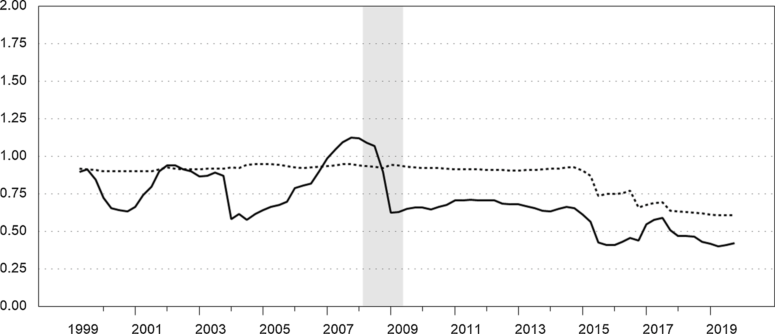
Figure 6. Morishima elasticities of substitution for changes in the user cost of NIBM. Quarterly. The solid series is $ME_{13}$
. The dotted series is
$ME_{13}$
. The dotted series is $ME_{12}$
. Recession is shaded.
$ME_{12}$
. Recession is shaded.
We conclude that substitution between NIBM and sight and time deposits, respectively, in response to changes in the user cost of NIBM, as measured by $ME_{12}$
and
$ME_{12}$
and $ME_{13}$
, is inelastic over all or almost all of our sample, which implies that conventional simple sum monetary aggregates would be highly misleading economic indicators since they require all monetary assets to be perfect substitutes. In contrast, the most elastic substitution corresponds to
$ME_{13}$
, is inelastic over all or almost all of our sample, which implies that conventional simple sum monetary aggregates would be highly misleading economic indicators since they require all monetary assets to be perfect substitutes. In contrast, the most elastic substitution corresponds to $ME_{21}$
, which measures substitution between NIBM and interest-bearing MFI sight deposits in response to changes in the user cost of sight deposits. Substitution between sight and time deposits in response to changes in the user cost of sight deposits as measured by
$ME_{21}$
, which measures substitution between NIBM and interest-bearing MFI sight deposits in response to changes in the user cost of sight deposits. Substitution between sight and time deposits in response to changes in the user cost of sight deposits as measured by $ME_{23}$
is also generally elastic except in the last several years of our sample.
$ME_{23}$
is also generally elastic except in the last several years of our sample.
5. Household-sector Divisia aggregates for the UK
The Bank of England’s Divisia measures are based on the following formula (Hancock, Reference Hancock2005):
 \begin{equation}\frac{{\Delta} D_{t}}{D_{t-1}}=\sum _{i}\left(\frac{s_{i,t}+s_{i,t-1}}{2}\right)\frac{{\Delta} M_{i,t}}{M_{i,t-1}}\end{equation}
where $s_{i,t}=\frac{(R_{t}-r_{i,t})M_{i,t}}{\sum _{j}(R_{t}-r_{j,t})M_{j,t}}$
is the expenditure share of the
$s_{i,t}=\frac{(R_{t}-r_{i,t})M_{i,t}}{\sum _{j}(R_{t}-r_{j,t})M_{j,t}}$
is the expenditure share of the $i$
th monetary asset. Thus, the growth rates of the Divisia measures weight the growth rates of the component monetary assets by their average expenditure shares. The expenditure shares of NIBM exceed their weights within a corresponding simple sum monetary aggregate as discussed, for example, by Anderson et al. (Reference Anderson, Duca, Fleissig and Jones2019). The Bank of England calculates the Divisia measures using non-break-adjusted levels,
$i$
th monetary asset. Thus, the growth rates of the Divisia measures weight the growth rates of the component monetary assets by their average expenditure shares. The expenditure shares of NIBM exceed their weights within a corresponding simple sum monetary aggregate as discussed, for example, by Anderson et al. (Reference Anderson, Duca, Fleissig and Jones2019). The Bank of England calculates the Divisia measures using non-break-adjusted levels, $M_{i,t}$
, but using break-adjusted flows,
$M_{i,t}$
, but using break-adjusted flows, $F_{i,t}$
, to measure
$F_{i,t}$
, to measure ${\Delta} M_{i,t}$
as explained by Hancock (Reference Hancock2005).
${\Delta} M_{i,t}$
as explained by Hancock (Reference Hancock2005).
Following the same approach, we constructed a household-sector Divisia aggregate corresponding to the components of our demand system model based on the user costs described in Section 2.2 using monthly data on the flows and amounts outstanding of notes and coin, noninterest-bearing deposits, interest-bearing MFI sight deposits, and MFI time deposits. Figure 7 compares the annual growth rates of this Divisia aggregate with those of the Bank of England’s monthly household-sector Divisia aggregate. The Bank of England’s household-sector Divisia aggregate places a positive expenditure share weight on the growth rate of TESSAs after ISAs are introduced in 1999, although the share was “low and declines rapidly” through the first quarter of 2004 after which TESSA balances are zero; see Elger et al. (Reference Elger, Jones, Edgerton and Binner2008, p. 122). We compare the annual growth rates of these aggregates beginning in April 2005, since our aggregate does not include TESSAs. The growth rates of the two Divisia aggregates are similar, but the growth rates of our Divisia aggregate are generally lower than that of the Bank of England’s Divisia measure following the recession. For the Bank of England’s measure, when the interest rate on ISAs falls below the upper envelope, the expenditure share of ISAs becomes positive and the growth rate of ISAs receives a positive weight in the growth rate of the aggregate, whereas the user cost of the component with the highest own rate becomes zero. In contrast, our aggregate does not include ISAs and the user costs underlying it are always positive.Footnote 18 Evidently, the Divisia aggregate is fairly robust over this period in that it is not greatly impacted by these differences related to the user costs and the differential treatment of ISAs.
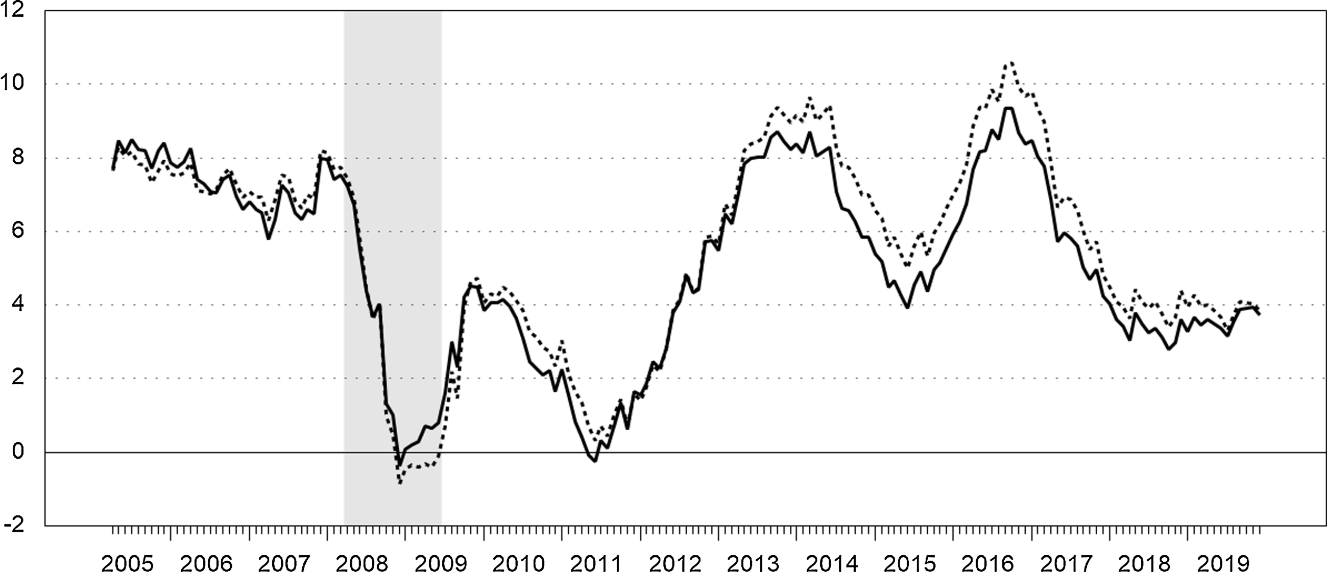
Figure 7. Annual growth rates of household-sector Divisia measures. Monthly. Annual growth rates, $(D_{t}-D_{t-12})/D_{t-12}$
, as a percentage. The solid series is the Divisia aggregate corresponding to the components of our demand system model based on the user costs described in Section 2.2. The dotted series is the Bank of England’s household-sector Divisia measure. Recession is shaded.
$(D_{t}-D_{t-12})/D_{t-12}$
, as a percentage. The solid series is the Divisia aggregate corresponding to the components of our demand system model based on the user costs described in Section 2.2. The dotted series is the Bank of England’s household-sector Divisia measure. Recession is shaded.
Figure 8 compares the annual growth rates of our household-sector Divisia aggregate to those of the corresponding simple sum monetary aggregate for the components of our demand system over the same period as the previous figure. These aggregates exhibit very different annual growth rates during the period surrounding the global financial crisis. Annual growth of the household-sector Divisia aggregate was generally below that of the simple sum in the period leading up to the 2008–2009 recession and during the recession. There was a steep decline in the user cost of NIBM during the recession and the annual growth rate of Divisia turned slightly negative, while the simple sum aggregate’s annual growth rate declined but remained positive throughout the recession. Along the same lines, Rayton and Pavlyk (Reference Rayton and Pavlyk2010) found that annual growth of the Bank of England’s broader Divisia M4 measure was barely positive during the same period, while growth of the corresponding simple sum M4 aggregate had “nearly doubled in the last year.” Immediately following the recession, however, our household-sector Divisia aggregate grew at higher annual rates than the simple sum aggregate. We also find that the simple sum aggregate understated annual money growth relative to our Divisia aggregate throughout the period from 2013 to 2018. The spread between the annual growth rates of the aggregates gradually narrowed from 2014 on with the annual growth rates of the two aggregates converging in 2019.

Figure 8. Annual growth rates of household-sector Divisia and simple sum aggregates. Monthly. Annual growth rates, $(D_{t}-D_{t-12})/D_{t-12}$
, as a percentage. The solid series is the Divisia aggregate corresponding to the components of our demand system model based on the user costs described in Section 2.2. The dotted series is the corresponding simple sum monetary aggregate. Recession is shaded.
$(D_{t}-D_{t-12})/D_{t-12}$
, as a percentage. The solid series is the Divisia aggregate corresponding to the components of our demand system model based on the user costs described in Section 2.2. The dotted series is the corresponding simple sum monetary aggregate. Recession is shaded.
To gain additional insight into the role of money in the UK economy, we estimate backward-looking models based on Elger et al. (Reference Elger, Jones, Edgerton and Binner2008) and Bissoondeeal et al. (Reference Bissoondeeal, Karogloua and Binner2019). Bissoondeeal et al. (Reference Bissoondeeal, Karogloua and Binner2019) estimated a backward-looking IS curve equation of the following form:
 \begin{equation}\tilde{g}_{t}=\beta _{0}+\beta _{1}\tilde{g}_{t-1}+\beta _{2}\tilde{g}_{t-2}+\gamma \tilde{r}_{t-1}+\varphi {\Delta} _{4}m_{t-1}+\varepsilon _{t}\end{equation}
using quarterly UK data from 1977 to 2013, where $\tilde{g}_{t}$
is the output gap,
$\tilde{g}_{t}$
is the output gap, $\tilde{r}_{t}$
is a smoothed real interest rate variable, and
$\tilde{r}_{t}$
is a smoothed real interest rate variable, and ${\Delta} _{4}m_{t}$
is the annual change in the log of a real money measure.Footnote
19
For the money measures, they used the UK Divisia and simple sum M4 aggregates, and they measured the output gap by detrending the log of real GDP using both the HP and Hamilton filters and by estimating a quadratic time trend. For the real interest rate, they used the four-quarter average of a Treasury bill rate minus annual inflation based on the consumer price index (CPI), which they also use to convert money and nominal output to real terms. Bissoondeeal et al. (Reference Bissoondeeal, Karogloua and Binner2019) tested for breaks in the data over the sample and estimated the model over three shorter samples based on the results. They identify breaks related to three events: “a recession in early 1980s, the UK exiting the ERM [exchange rate mechanism] in 1992 and the recent financial crisis” (p. 103).
${\Delta} _{4}m_{t}$
is the annual change in the log of a real money measure.Footnote
19
For the money measures, they used the UK Divisia and simple sum M4 aggregates, and they measured the output gap by detrending the log of real GDP using both the HP and Hamilton filters and by estimating a quadratic time trend. For the real interest rate, they used the four-quarter average of a Treasury bill rate minus annual inflation based on the consumer price index (CPI), which they also use to convert money and nominal output to real terms. Bissoondeeal et al. (Reference Bissoondeeal, Karogloua and Binner2019) tested for breaks in the data over the sample and estimated the model over three shorter samples based on the results. They identify breaks related to three events: “a recession in early 1980s, the UK exiting the ERM [exchange rate mechanism] in 1992 and the recent financial crisis” (p. 103).
In line with our focus on household-sector money demand, we estimate equation (6) using detrended real consumption rather than GDP. Specifically, real consumption is the quarterly seasonally adjusted chained volume measure for total UK national household final consumption expenditure from Consumer Trends (Office for National Statistics). To calculate $\tilde{g}_{t}$
, we detrended the natural log of real consumption using the same three methods that Bissoondeeal et al. (Reference Bissoondeeal, Karogloua and Binner2019) used for real GDP.Footnote
20
The real interest rate is defined as
$\tilde{g}_{t}$
, we detrended the natural log of real consumption using the same three methods that Bissoondeeal et al. (Reference Bissoondeeal, Karogloua and Binner2019) used for real GDP.Footnote
20
The real interest rate is defined as $\tilde{r}_{t}=\sum _{j=0}^{3}R_{t-j}-{\Delta} _{4}p_{t}$
, where
$\tilde{r}_{t}=\sum _{j=0}^{3}R_{t-j}-{\Delta} _{4}p_{t}$
, where $R_{t}$
is a short-term nominal interest rate (as a quarterly fraction of the annual rate) and
$R_{t}$
is a short-term nominal interest rate (as a quarterly fraction of the annual rate) and $p_{t}$
is the natural log of a price index; see, for example, Binner et al. (2009, p. 105). We use a quarterly average rate on 3-month Treasury bills, which is available until 2017. This, in turn, determines the end point of our sample period for the estimations. For
$p_{t}$
is the natural log of a price index; see, for example, Binner et al. (2009, p. 105). We use a quarterly average rate on 3-month Treasury bills, which is available until 2017. This, in turn, determines the end point of our sample period for the estimations. For $p_{t}$
, we calculate a deflator corresponding to the measure of real consumption described above, which we also use to convert the monetary aggregates to real terms.
$p_{t}$
, we calculate a deflator corresponding to the measure of real consumption described above, which we also use to convert the monetary aggregates to real terms.
We estimate a baseline version of the model that omits lagged annual real money growth, ${\Delta} _{4}m_{t-1}$
, and we estimate the model using the Bank of England’s quarterly household-sector Divisia series, which is available beginning in 1977. We also estimate the model using a quarterly household-sector Divisia aggregate that we constructed over the same period, which is based on a benchmark rate equal to the highest own rate plus 60 basis points. Beginning in 1999, this series corresponds to quarterly averages of the monthly Divisia series we constructed above; see Appendix B for further details. For comparison purposes, we also estimated the model using a simple sum aggregate. The Bank of England publishes quarterly series on the outstanding amount of M4 liabilities to the household sector and corresponding quarterly changes.Footnote
21
We constructed a corresponding break-adjusted series from these data using the same method described in Section 2.1, and we estimated the models using this series as well. The results are reported in Table 3, where D1 indicates results based on the Divisia aggregate we constructed, D2 indicates results for the Bank of England’s household-sector Divisia aggregate, and SUM indicates results for break-adjusted M4 liabilities to the household sector. The effective sample period is 1978Q2 to 2017Q2 due to the inclusion of lagged real Divisia money growth.
${\Delta} _{4}m_{t-1}$
, and we estimate the model using the Bank of England’s quarterly household-sector Divisia series, which is available beginning in 1977. We also estimate the model using a quarterly household-sector Divisia aggregate that we constructed over the same period, which is based on a benchmark rate equal to the highest own rate plus 60 basis points. Beginning in 1999, this series corresponds to quarterly averages of the monthly Divisia series we constructed above; see Appendix B for further details. For comparison purposes, we also estimated the model using a simple sum aggregate. The Bank of England publishes quarterly series on the outstanding amount of M4 liabilities to the household sector and corresponding quarterly changes.Footnote
21
We constructed a corresponding break-adjusted series from these data using the same method described in Section 2.1, and we estimated the models using this series as well. The results are reported in Table 3, where D1 indicates results based on the Divisia aggregate we constructed, D2 indicates results for the Bank of England’s household-sector Divisia aggregate, and SUM indicates results for break-adjusted M4 liabilities to the household sector. The effective sample period is 1978Q2 to 2017Q2 due to the inclusion of lagged real Divisia money growth.
Table 3. Effects of household-sector monetary aggregates on real consumption
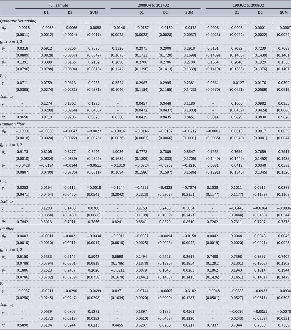
Note: The full sample period is 1978Q2 to 2017Q2. D1 denotes the household-sector Divisia aggregate based on a benchmark rate equal to the upper envelope of the own rates plus 60 basis points (see Appendix B for details). D2 denotes the Bank of England’s household-sector Divisia aggregate. SUM denotes the break-adjusted series for M4 liabilities to the household sector. Standard errors for parameter estimates are in parentheses.
We find evidence of direct effects of the household-sector money measures on real consumption for the full sample for all three detrending methods. Specifically, we find that the coefficient on lagged real money growth is positive and statistically significant at the 1% level for both Divisia aggregates for all three detrending methods for the full sample. The coefficient on lagged real money growth is also positive and statistically significant at the 1% level for the simple sum aggregate for quadratic detrending and for the HP filter, but it is not statistically significant for the Hamilton filter.Footnote 22 These results are similar to Bissoondeeal et al. (Reference Bissoondeeal, Karogloua and Binner2019) who found for their full sample that Divisia M4 was statistically significant in their regressions based on GDP using all three detrending methods, but that simple sum M4 was only statistically significant at the 5% level for the HP filter, although it was close for quadratic detrending.
Bissoondeeal et al. (Reference Bissoondeeal, Karogloua and Binner2019) also estimated their model over three subsamples: 1982Q1 to 1991Q3, 1993Q2 to 2008Q2, and from 2008Q4 through the end of their sample period (2013Q4). They found that Divisia and simple sum M4 were both significant in the first subsample for all three detrending methods, but that only Divisia M4 was significant in the latter two subsamples and in each one only for two of the three detrending methods. We also estimated our model over the corresponding subsamples. We report results for 1993Q2 to 2008Q2 and for 2008Q4 to 2017Q2 in Table 3, but we do not show the results from the earlier subsample to save space. For 1982Q1 to 1991Q3, we found that the coefficient on lagged real money growth is positive and statistically significant at the 5% level for both Divisia aggregates for quadratic detrending and the Hamilton filter and at the 10% level for the HP filter.Footnote 23 For 1993Q2 to 2008Q2, the coefficient on lagged real money growth is positive and statistically significant at the 5% level for both Divisia aggregates for quadratic detrending, but it is not significant for either Divisia aggregate for the other two detrending methods and the estimated coefficients are negative. With regard to real money growth, the results for this subsample are evidently not robust to the detrending method, but the results for quadratic detrending are generally in line with the results discussed previously. For the simple sum aggregate, the coefficient on lagged real money growth is not statistically significant for either the 1982Q1 to 1991Q3 or 1993Q2 to 2008Q2 subsamples for any of the three detrending methods. For 2008Q4 to 2017Q2, the coefficient on lagged real money growth is positive and statistically significant at the 5% level for all three monetary aggregates for the Hamilton filter and at the 1% level for the HP filter, but it is not statistically significant for any of the three monetary aggregates for quadratic detrending.
Taken together, our results for real consumption point to the advantages of using a Divisia aggregate relative to conventional monetary aggregates similar to the results from Bissoondeeal et al. (Reference Bissoondeeal, Karogloua and Binner2019) for GDP. The growth rates of the Divisia aggregates are both highly statistically significant in our model for the full sample for all three detrending methods, and they are both statistically significant for at least one of the detrending methods in each of the three subsamples. In contrast, the growth rate of the simple sum aggregate is only statistically significant for the full sample for two of the three detrending methods and is not significant in two of the three subsamples for any of the three detrending methods.
Elger et al. (Reference Elger, Jones, Edgerton and Binner2008) estimated a model for the output gap incorporating four lags of quarterly real money growth. Their model is as follows:
 \begin{equation}\tilde{g}_{t}=\beta _{0}+\sum _{k=1}^{4}\beta _{k}\tilde{g}_{t-k}+\sum _{k=1}^{4}\gamma _{k}\tilde{r}_{t-k}+\sum _{k=1}^{4}\theta _{k}{\Delta} m_{t-k}+\varepsilon _{t}\end{equation}
where $\tilde{r}_{t}$
is defined in the same way as above and
$\tilde{r}_{t}$
is defined in the same way as above and ${\Delta} m_{t}$
denotes the quarterly change in the log of a real money measure. Elger et al. (Reference Elger, Jones, Edgerton and Binner2008) measured the output gap as deviations of the log of real GDP from an estimated quadratic time trend. They found strong evidence of direct effects for four household-sector Divisia aggregates and the monetary base, but they also noted (pp. 127–128) that “the improvement in fit from the model that omits money to the best fitting specification that includes real money growth… is very modest” in terms of
${\Delta} m_{t}$
denotes the quarterly change in the log of a real money measure. Elger et al. (Reference Elger, Jones, Edgerton and Binner2008) measured the output gap as deviations of the log of real GDP from an estimated quadratic time trend. They found strong evidence of direct effects for four household-sector Divisia aggregates and the monetary base, but they also noted (pp. 127–128) that “the improvement in fit from the model that omits money to the best fitting specification that includes real money growth… is very modest” in terms of $R^{2}$
.Footnote
24
We estimate equation (7) over the full sample (1978Q2 to 2017Q2) for the detrended log of real consumption using all three detrending methods described above, and the results are reported in Table 4.
$R^{2}$
.Footnote
24
We estimate equation (7) over the full sample (1978Q2 to 2017Q2) for the detrended log of real consumption using all three detrending methods described above, and the results are reported in Table 4.
Table 4. Effects of household-sector monetary aggregates on real consumption
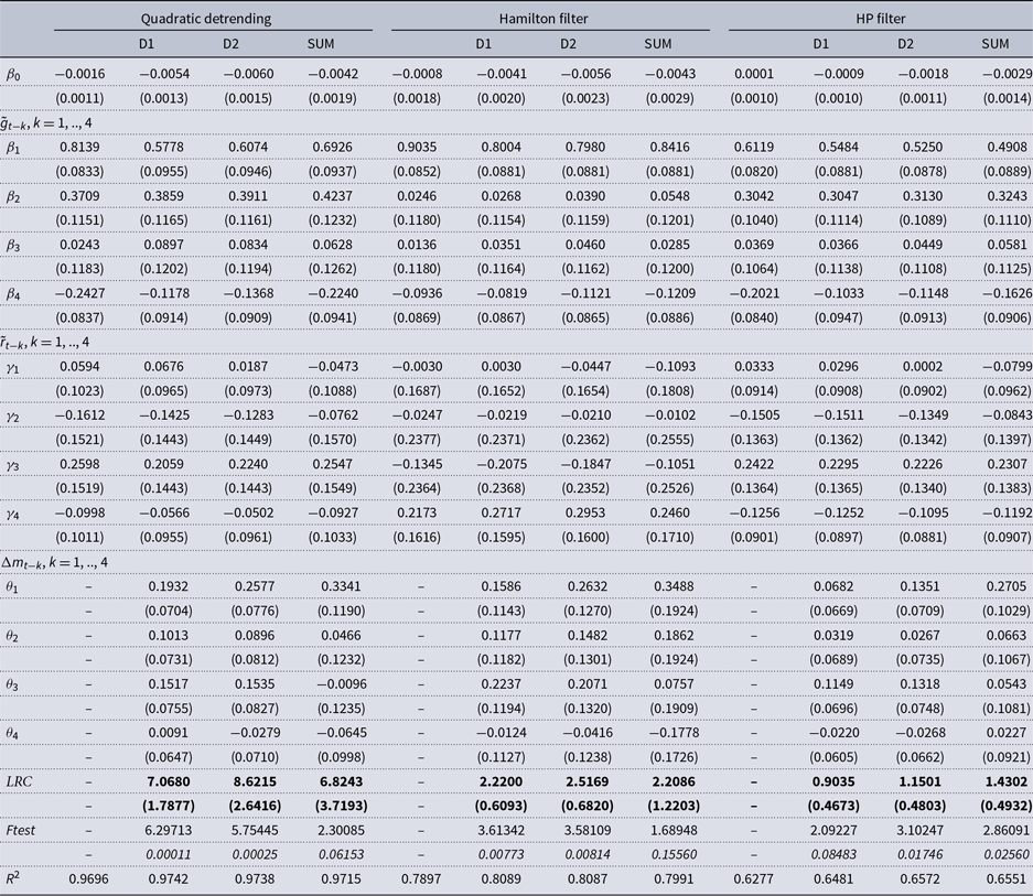
Note: D1 denotes the household-sector Divisia aggregate based on a benchmark rate equal to the upper envelope of the own rates plus 60 basis points (See Appendix B for details). D2 denotes the Bank of England’s household-sector Divisia aggregate. SUM denotes the break-adjusted series for M4 liabilities to the household sector. Standard errors for parameter estimates are in parentheses. $\mathrm{LRC}=\sum _{k}\theta _{k}/(1-\sum _{k}\beta _{k})$
. F-test is the test statistic for joint significance of the four money growth terms. The significance level is in italics.
$\mathrm{LRC}=\sum _{k}\theta _{k}/(1-\sum _{k}\beta _{k})$
. F-test is the test statistic for joint significance of the four money growth terms. The significance level is in italics.
We find evidence of direct effects of the real household-sector money measures for this specification as well for all three detrending methods. For quadratic detrending, the four lags of real money growth are jointly significant at the 1% level for both Divisia aggregates. The corresponding long-run coefficients on real money growth ( $LRC$
) are 7.068 for the Divisia aggregate we constructed and 8.622 for the Bank of England’s Divisia aggregate, which can be compared to estimates for the Divisia aggregates from Elger et al. (Reference Elger, Jones, Edgerton and Binner2008) ranging from 3.225 to 3.932 with their highest LRC corresponding to the Bank of England’s household-sector Divisia aggregate. For the simple sum aggregate, the four lags are jointly significant at the 10% level and the corresponding long-run coefficient is 6.824. The four lags of real money growth are also jointly significant at the 1% level for both Divisia aggregates for the Hamilton filter, and the corresponding long-run coefficients are 2.220 and 2.517. The four lags are not jointly significant for the simple sum aggregate for the Hamilton filter. For the HP filter, the four lags of real money growth are jointly significant at the 5% level for the Bank of England’s Divisia aggregate and for the simple sum aggregate. They are jointly significant at the 10% level for the Divisia aggregate we constructed, and the corresponding LRC are 1.150, 1.430, and 0.904, respectively.
$LRC$
) are 7.068 for the Divisia aggregate we constructed and 8.622 for the Bank of England’s Divisia aggregate, which can be compared to estimates for the Divisia aggregates from Elger et al. (Reference Elger, Jones, Edgerton and Binner2008) ranging from 3.225 to 3.932 with their highest LRC corresponding to the Bank of England’s household-sector Divisia aggregate. For the simple sum aggregate, the four lags are jointly significant at the 10% level and the corresponding long-run coefficient is 6.824. The four lags of real money growth are also jointly significant at the 1% level for both Divisia aggregates for the Hamilton filter, and the corresponding long-run coefficients are 2.220 and 2.517. The four lags are not jointly significant for the simple sum aggregate for the Hamilton filter. For the HP filter, the four lags of real money growth are jointly significant at the 5% level for the Bank of England’s Divisia aggregate and for the simple sum aggregate. They are jointly significant at the 10% level for the Divisia aggregate we constructed, and the corresponding LRC are 1.150, 1.430, and 0.904, respectively.
6. Conclusion
We estimated Morishima elasticities of substitution between UK household-sector monetary assets based on a Fourier demand system for the first two decades of the new Millennium. The estimated demand model covers the period from 1999 to 2019. Accounting for recent changes in the data underlying the Bank of England’s Divisia measures, our analysis is based on three components: NIBM, interest-bearing MFI sight deposits, and MFI time deposits. We found that the Morishima elasticities that are most relevant to monetary policy are the ones that capture substitution in response to changes in the user cost of NIBM. These elasticities imply inelastic substitution over all or almost all of the sample period, which in turn implies that conventional monetary aggregates are highly misleading economic indicators. The highest elasticities are the ones that capture substitution in response to changes in the user cost of MFI sight deposits. The components of our model necessarily differ somewhat from those of Drake et al. (Reference Drake, Fleissig and Swofford2003) given changes in the data over time, but we find some similarities to their results with respect to asymmetry of the estimated Morishima elasticities.
Simple sum monetary aggregates require all included monetary assets to be perfect substitutes, which is ultimately an empirical issue. Our finding that the Morishima elasticities of substitution are generally inelastic except for the ones that capture substitution in response to changes in the user cost of sight deposits implies that a conventional monetary aggregate would be a poor economic indicator relative to a Divisia aggregate. Building on Elger et al. (Reference Elger, Jones, Edgerton and Binner2008) and Bissoondeeal et al. (Reference Bissoondeeal, Karogloua and Binner2019), we estimated backward-looking models of detrended real consumption that include lagged growth rates of real household-sector Divisia and simple sum monetary aggregates using three different detrending methods. For the specification based on Bissoondeeal et al. (Reference Bissoondeeal, Karogloua and Binner2019), we found evidence of direct effects of real money growth for two household-sector Divisia aggregates for the full sample period from 1977 to 2017 for all three detrending methods and for at least one of the three detrending methods in each of the three subsamples we considered. In contrast, the results for the simple sum monetary aggregate were somewhat weaker for this specification in that the simple sum was only significant for the full sample period for two of the three detrending methods and was not significant in two of the three subsamples for any of the three detrending methods.
Acknowledgments
The authors thank the Editor, Associate Editor, and three anonymous referees for helpful comments and suggestions that greatly improved the paper. We also thank the Office for National Statistics for answering questions related to Consumer Trends data.
Appendix A: Break-adjusted components
We estimate the Fourier model using break-adjusted series for NIBM and MFI sight and time deposits. We provide more detailed explanations regarding the data in this appendix. The break-adjusted series are based on seasonally adjusted data. Monthly break-adjusted series for notes and coin (N&C) and noninterest-bearing deposits (NIBD) can be constructed back to September 1997 from available data on flows and amounts outstanding from the Bank of England. To compute an index for NIBM, we apply the formula described in Section 2 to the sum of the flows for N&C and NIBD and to the corresponding sum of the amounts outstanding.Footnote 25
As discussed previously, the Bank of England published separate data for banks and building societies up through December 2009, which were used to calculate the Divisia series (see Berar, Reference Berar2013). As Berar (Reference Berar2013) explains, beginning in January 2010, the Bank published separate data for banks (excluding mutuals) and for mutuals. These separate data were discontinued after November 2013, and only MFI series were published subsequently (see Bailey, Reference Bailey2014).
For sight and time deposits, we construct break-adjusted indexes using the MFI series as far back as possible (January 2008). We then extend these indexes back to December 1998 using the available disaggregate data for these components for banks and building societies. To do this, we apply the formula from Section 2 to the sum of the flows at banks and building societies and to the corresponding sum of the amounts outstanding for the relevant periods.
Appendix B: Quarterly household-sector Divisia aggregate
We estimated backward-looking models for detrended real consumption using a quarterly household-sector Divisia series beginning in 1977 based on a benchmark rate equal to the highest own rate plus 60 basis points. We provide more details regarding this series in this appendix.
Beginning in 1999, this series is the quarterly average of the monthly Divisia aggregate we constructed in Section 5, which corresponds to the components of our demand system model based on the user costs described in Section 2.2.
For earlier periods, we constructed a household-sector Divisia aggregate using quarterly, seasonally adjusted, data from 1977Q1 to 1999Q1 on the flows and amounts outstanding of notes and coin, noninterest-bearing deposits, sight deposits at banks, time deposits at banks, and building society deposits.Footnote 26 The own rates for the interest-bearing components are quarterly series on household-sector quoted rates for interest-bearing bank sight deposits, interest-bearing bank time deposits, and building society deposits, respectively.Footnote 27 We define the benchmark rate as the maximum of these three own rates plus a liquidity premium of 60 basis points.Footnote 28 We found that the maximum rate alternates between the bank time deposit rate and the building society rate, but it is consistently the bank time deposit rate beginning in 1994Q4. The resulting quarterly Divisia series is spliced to the one beginning in 1999 (based on quarterly averages of the monthly Divisia series we constructed in Section 5) to produce a series for the full sample period beginning in 1977.


