3.1. The $Pr$ dependence of the flow topology evolution

We first compare the flow topology at different values of $Pr$. Figure 1 presents the velocity field obtained through PIV measurements, averaged over a short time period, at $Pr = 7.0$, $128.5$ and $244.2$, respectively, within the similar range of $Ra$. The short-time averaged velocity fields presented here are essentially instantaneous snapshots. The purpose of applying a short-time average to the instantaneous snapshots is to enhance the clarity of the flow field. However, it is important to note that even with this short-time averaging, the flow fields maintain their instantaneous nature, albeit with a clearer and more distinct flow topology. During averaging process, we ensured that there were no flow reversals within the short time period. As an instantaneous velocity map may not reflect the main feature of the flow, the selection of the short-time averaged velocity maps is based on the mean flow structure, i.e. the dominant Fourier mode from the time average of all the flow modes of the entire PIV measurement at each $Ra$ (usually lasts for 2–3 hours), which is presented in figure 2. If the single-roll formed LSC exists, then the short time period used for averaging corresponds to one turnover time of the LSC. In cases where there is no LSC but the flow exhibits multicellular structures, the short time period is determined by the typical circulation time of a cellular flow structure. In fact, the multicellular flow structure remains quite stable for an extended duration in our experiments, making the choice of the average time less critical. For $Pr = 7.0$, figures 1(a,d,g,j,m) illustrate a typical transition in flow topology from an abnormal single-roll state (ASRS) (figure 1a) to a single-roll state (SRS) (figures 1d,g,j,m), as previously observed by Chen et al. (Reference Chen, Huang, Xia and Xi2019). The ASRS is characterized by the presence of a large vortex in the flow field, with the interior of this vortex splitting into two smaller vortices. The formation of substructures within the large vortex arises from the balance between plume travel and plume dissipation time. The SRS, commonly observed in earlier studies (Xia et al. Reference Xia, Sun and Zhou2003; Sugiyama et al. Reference Sugiyama, Ni, Stevens, Chan, Zhou, Xi, Sun, Grossmann, Xia and Lohse2010), consists of a main vortex with two small corner vortices in the tilted-ellipse shape.

Figure 1. Short-time averaged PIV velocity maps with streamlines for different $Ra$ and $Pr$, where $u$ and $w$ are horizontal and vertical components of the velocity: (a,d,g,j,m) $Pr = 7.0$, (b,e,h,k,n) $Pr =128.5$, (c,f,i,l,o) $Pr = 244.2$.

Figure 2. (a–f) Cartoon patterns of the six Fourier modes of the velocity fields. (g–i) Time-averaged energy contained in each flow mode as a function of $Ra$ for $Pr = 7.0, 128.5, 244.2$, respectively. The dashed line represents the value of $Ra$ where the crossover between $(2,2)$ mode and $(1,1)$ mode occurs (i.e. $Ra_{t}$).

As $Pr$ is increased to 128.5, the flow topology exhibits distinct difference compared with the $Pr = 7.0$ case, as shown in figures 1(b,e,h,k,n). At $Ra = 2 \times 10^8$, the mean field displays a side-by-side four-roll state (sFRS) (figure 1b). This state is characterized by the presence of four slender rolls arranged horizontally adjacent to each other within the flow. For $Ra = 4.01 \times 10^8$, the flow is dominated by strong vertical motions and exhibits a double-roll state (DRS) (figure 1e), with downward flow at the centre of the cell, and upward flow near the sidewalls. It is worthwhile to note that during the measurement time, no reversal is observed for the sFRS and the DRS. Further increasing $Ra$ to $7.42 \times 10^8$, the mean field transitions to a distinct four-roll state (FRS), diverging from the aforementioned sFRS. Earlier studies suggested that the FRS could arise from the superposition of two LSC flow fields with opposite directions due to frequent flow reversals (Chong et al. Reference Chong, Wagner, Kaczorowski, Shishkina and Xia2018). However, in this study, all flow fields are averaged within a short time interval, during which no flow reversal occurs. The FRS is quite stable; even when averaging the flow field over the entire measurement period, it remains in the FRS. As $Ra$ is increased further, the flow topology transitions from FRS to ASRS and eventually to SRS, similar to the case $Pr = 7.0$. To the best of our knowledge, this is the first observation of sFRS and DRS in a convection cell with $\varGamma =1$. Another important finding is that the transitional $Ra$ corresponding to the transition from ASRS to SRS differs between $Pr = 7.0$ and $Pr = 128.5$. For $Pr = 7.0$, the transition occurs between $Ra = 2.29 \times 10^8$ (figure 1a) and $Ra = 5.13 \times 10^8$ (figure 1d), while for $Pr = 128.5$, it occurs between $Ra = 1.22 \times 10^9$ (figure 1k) and $Ra = 1.48 \times 10^9$ (figure 1n). This suggests that a higher $Ra$ is required to establish a well-defined LSC at higher $Pr$.

As $Pr$ increases to 244.2, the evolution of flow topology follows a different route compared to the cases $Pr = 7$ and $Pr = 128.5$. With increasing $Ra$, the flow field gradually transitions from FRS to DRS. In the FRS, the two upper rolls progressively grow in size and compress the two lower rolls until $Ra = 1.0 \times 10^9$, where the two upper rolls occupy nearly the entire cell. The DRS persists throughout our experiments, even at the highest $Ra$ values. Interestingly, the DRS observed at $Pr = 244.2$ has the direction opposite to that observed at $Pr = 128.5$ (figure 1e). Furthermore, the direction of the DRS remains consistent throughout current measurement, which lasts for almost 2 days. A similar DRS flow field was reported by Li et al. (Reference Li, He, Tian, Hao and Huang2021) at $Ra = 1.4 \times 10^{10}$ and $Pr = 345.2$ using shadowgraph visualization. They observed clusters of plumes rising from the middle of the lower plate in the convection cell. However, we currently lack an understanding of the differences between these two types of DRS (figures 1e,o) and whether a flow reversal also exists in the DRS. This aspect certainly demands further investigation in future studies.

To qualitatively analyse the flow topology, we examine the flow energy using Fourier mode decomposition (Chandra & Verma Reference Chandra and Verma2011; Wagner & Shishkina Reference Wagner and Shishkina2013; Chong et al. Reference Chong, Wagner, Kaczorowski, Shishkina and Xia2018). In this approach, each instantaneous velocity field ($u_{x}, u_{z}$) is projected onto the Fourier modes as follows:

(3.1)$$\begin{gather} u_{x}^{m, n}=2 \sin (m {\rm \pi}x) \cos (n {\rm \pi}z), \end{gather}$$

(3.2)$$\begin{gather}u_{z}^{m, n}={-}2 \cos (m {\rm \pi}x) \sin (n {\rm \pi}z). \end{gather}$$

Typically the first four modes are considered (i.e. $m,n = 1, 2$). In this study, considering the observed sFRS, we also include the modes with $m = 3, 4$ and $n = 1$. The instantaneous amplitude of each mode $A^{m, n}(t)$ is obtained by projecting the velocity field components onto the corresponding Fourier modes: $A^{m, n}(t) = \langle u_{x}(t)\,u_{x}^{m, n}\rangle _{x, z} + \langle u_{z}(t)\,u_{z}^{m, n}\rangle _{x, z}$. Consequently, the energy of each flow mode can be evaluated as $E^{m, n}(t) = [A^{m, n}(t)]^2$ (Xi et al. Reference Xi, Zhang, Hao and Xia2016).

Figures 2(g–i) show the mean energy contained in each of the six Fourier modes as a function of $Ra$. Here, the mean energy contained within each of the six Fourier modes is computed by averaging over the entire measurement period. For $Pr = 7.0$, the $(1,1)$ and $(2,2)$ modes contain the majority of the energy, while the $(1,2)$, $(3,1)$ and $(4,1)$ modes remain negligibly weak throughout the entire range of $Ra$. As $Ra$ increases, the energy of the $(2,2)$ mode decreases, while the energy of the $(1,1)$ mode increases. There exists a crossover $Ra$ value ($Ra_{t}$) between the $(2,2)$ mode and the $(1,1)$ mode. When $Ra$ is below $Ra_{t}$, the $(2,2)$ mode dominates the flow field, but the $(1,1)$ mode remains comparable. In this situation, the flow field corresponds to the ASRS. When $Ra$ is larger than $Ra_t$, the $(1,1)$ mode surpasses the $(2,2)$ mode and becomes dominant, resulting in the flow transition to the SRS.

As $Pr$ increases to 128.5 (figure 2h), the evolution of each mode with $Ra$ becomes more complex. For the lowest $Ra$, the $(4,1)$ mode has the highest energy among all modes, consistent with the sFRS flow field shown in figure 1(b). As $Ra$ further increases, the $(4,1)$ mode is surpassed by the $(2,1)$ mode, which dominates the flow field until the $(2,2)$ mode overtakes the $(2,1)$ mode. Before this transition, the flow field corresponds to the DRS. Once the $(2,2)$ mode begins to dominate the flow field, the energy of the $(1,1)$ mode starts to increase rapidly with increasing $Ra$. When $Ra$ exceeds $Ra_t$, the $(1,1)$ mode becomes dominant, and the flow field eventually evolves from ASRS into the SRS. The evolution of the mode energy with $Ra$ shown in figure 2(h) is consistent with the flow field evolution illustrated in figure 1.

At $Pr = 244.2$ (figure 2i), the flow field undergoes a transition from dominance of the $(2,2)$ mode to dominance of the $(2,1)$ mode, which is consistent with the FRS to DRS transition observed in figure 1. Additionally, we observe that there exists a critical $Ra$ (approximately $Ra = 6 \times 10^8$) for the $(1,1)$ and $(2,2)$ modes. The values of the $(1,1)$ and $(2,2)$ modes remain almost unchanged when $Ra \leq 6 \times 10^8$. In contrast to the $(1,1)$ and $(2,2)$ modes, the value of the $(2,1)$ mode increases with increasing $Ra$, while the values of the $(3,1)$ and $(4,1)$ modes decrease. Although there are distinct differences in the evolution of each mode at different $Pr$, there is a one-to-one correspondence between the flow mode and the flow topology.

One may observe that in the cases with relative low $Ra$ at higher $Pr$, such as those shown in figures 1(b,c), the velocity fields are relatively chaotic, distinguishing them from cases with higher $Ra$. This distinction can be attributed to the results presented in figures 2(h,i), where for small $Ra$, several flow modes are comparable to each other in terms of the energy contained in each mode, thus the flow structure is a composition of the different flow modes, resulting in a relatively chaotic flow field. However, as $Ra$ increases, certain flow modes (e.g. $(1,1)$ or $(2,1)$) start to dominate the flow field more prominently than other modes, leading to a clearer and more distinct flow field. Concerning the flow fields shown in figures 1(b,c), we chose to make the average of the instantaneous snapshots over a short time period where the $(4,1)$ and $(2,2)$ modes dominate in the flow field compared to other flow modes, respectively. This method of selection ensures that the obtained flow field is a representative of the averaged (over the entire measurement) energy contained in each Fourier modes, i.e. a typical flow field at the specific control parameters.

We employ the dominance of the $(1,1)$ mode as the criterion for determining the existence of a well-defined LSC in the system, with the corresponding $Ra$ value denoted as the transitional $Ra$ ($Ra_t$). This transition is marked by the black dashed line in figures 2(g,h). Comparing figures 2(g) and 2(h), we observe that $Ra_t = 2.71 \times 10^8$ for $Pr = 7.0$, significantly smaller than $Ra_t = 1.12 \times 10^9$ for $Pr = 128.5$. This observation is in line with the fact that the transition from ASRS to SRS in figure 1 occurs at smaller $Ra$ for $Pr = 7.0$ compared to that for $Pr = 128.5$. In other words, a higher $Ra$ is required to form LSC for higher $Pr$. This may explain why we do not observe an LSC at $Pr = 244.2$, as the driving force ($Ra$) of the system may not be sufficient within the current range of $Ra$. We propose that the DRS is only a transitional state, and the LSC would likely emerge with further increase in $Ra$ at $Pr = 244.2$. However, the size of the current experimental set-up imposes limitations on further increasing $Ra$.

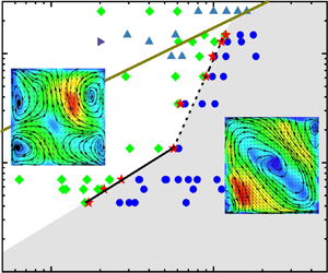
To further explore the influence of $Pr$ on the flow field, and examine the trend of $Ra_t$ on $Pr$, we extended the range of $Pr$ and constructed a phase diagram of dominant Fourier modes across a broad $Ra\unicode{x2013}Pr$ parameter space, as shown in figure 3. The phase diagram reveals that at low $Pr$, the system predominantly exhibits two modes: $(2,2)$ and $(1,1)$. As $Pr$ increases, new dominant modes emerge, namely $(4,1)$ and $(2,1)$, as shown in figures 1(b,e,l,o). The $Ra_t$ value, corresponding to the transition from the dominance of the $(2,2)$ mode to the $(1,1)$ mode, tends to increase with $Pr$. The increase of $Ra_t$ with increasing $Pr$ has two distinct regimes: a slow increase when $Pr \leq 13.5$, characterized by scaling slope 0.93, and a fast increase when $Pr \geq 13.5$, exhibiting a steeper scaling slope 3.3. To examine the scaling relationship between $Ra_t$ and $Pr$, Chen et al. (Reference Chen, Huang, Xia and Xi2019) proposed a time scale balance model in which the transition of the flow occurs when the plume kinetic energy dissipation (by viscosity) time is comparable to the time scale for the plume ascending or descending to the mid-height of the cell. This led to a scaling relationship $Ra_{t} \sim Pr^{1.06}$, closely matching their experimentally observed relationship $Ra_{t} \sim Pr^{1.12 \pm 0.07}$ within a narrow $Pr$ range $4.3 \leq Pr \leq 7.0$. In our current study, we validate the persistence of this scaling relationship between $Ra_{t}$ and $Pr$ in a wider $Pr$ range $Pr \leq 13.5$, with the scaling exponent being $1/0.93 = 1.08$, as shown by the black solid line in figure 3.

Figure 3. Phase diagram of the dominant Fourier modes in the $Ra\unicode{x2013}Pr$ parameter space. The stars indicate the transitional $Ra_t$. The black solid line and dashed line have slopes 0.93 and 3.3, respectively. The brown solid line is $Re = 50$, where $Re = 9.4 \times 10^{-3}\,Ra^{0.63}\, Pr^{-0.87}$ (see § 3.2 for description). The area above the brown solid line is where $Re \leq 50$. The shaded region represents the dominance of the $(1,1)$ mode. The data for $Pr = 4.3$, $5.7$ and $7.0$ from Chen et al. (Reference Chen, Huang, Xia and Xi2019) are also included.

As $Pr$ exceeds 13.5, the $Pr$ dependence of $Ra_t$ becomes less prominent compared to the moderate $Pr$ range. For instance, at $Pr = 13.5$, $Ra_t$ is $5.67 \times 10^8$, while at $Pr=148.3$, a tenfold increase, $Ra_t$ is increased only approximately twofold, i.e. $1.19 \times 10^9$, indicating a relatively small change in $Ra_t$ despite the substantial change in $Pr$. To explore this behaviour, we examine the Grashof number ($Gr = \alpha g\,{\rm \Delta} T\,H^3/\nu ^2 = Ra/Pr$), which represents the ratio of buoyancy to viscous forces (the corresponding $Gr\unicode{x2013}Pr$ phase diagram is provided in figure 8 in the Appendix). In our quasi-2-D study, the viscous force encompasses both internal fluid viscosity and the sidewall-induced viscous force. The previously deduced relationship $Ra_{t} \sim Pr^{1.06}$ at moderate $Pr$ can be expressed in terms of $Gr$ as $Gr_t \sim Pr^{0.06}$. The weak $Pr$ dependence of $Gr_t$ at moderate $Pr$ implies that the transitional $Gr_t$ remains relatively constant with varying $Pr$, indicating the existence of a critical $Gr$ threshold governing the transition from the dominance of the $(2,2)$ mode to the $(1,1)$ mode. Beyond this threshold, characterized by the nearly invariant $Gr_t$, the flow structure transforms into a single-roll form of the LSC or a $(1,1)$-mode-dominated flow field. The measured $Pr \sim Ra_{t}^{3.3}$ in the large $Pr$ range can also be expressed in terms of $Gr_t$ scaling as $Gr_t \sim Pr^{-0.7}$. In contrast to the small but positive exponent in the moderate $Pr$ range, the negative exponent at high $Pr$ indicates that with increasing $Pr$, the transitional $Gr_t$ decreases. From table 1, we can observe that the increase of $Pr$ is accompanied by an increase in viscosity, while thermal diffusivity remains relatively constant. In this high-$Pr$ regime ($Pr \geq 13.5$), $Gr$ is no longer approximately constant – i.e. the speed with which the buoyancy increases is slower than that of the viscous force – which suggests a different mechanism governing the formation of the $(1,1)$-dominated flow state. Indeed, the distinct mechanism observed in the high-$Pr$ regime merits deeper investigation in future studies.

3.2. The $Ra$ and $Pr$ dependence of the Reynolds number

As PIV provides direct measurement of the flow field, we can now investigate the $Ra$ and $Pr$ dependence of $Re$ more directly than in methods relying on local velocity measurements (Lam et al. Reference Lam, Shang, Zhou and Xia2002) or cross-correlation between adjacent thermistors (Li et al. Reference Li, He, Tian, Hao and Huang2021). In our study, we define the Reynolds number ($Re$) as $Re=\sqrt {\langle u^2+w^2 \rangle _{V,t}}\,H/\nu$, where $\langle \rangle _{V,t}$ represents the spatial average over the measuring plane and time average. Figure 4(a) shows the $Ra$ dependence of $Re$ at different $Pr$ based on the PIV velocity maps. First, we can observe a monotonic decrease in $Re$ with increasing $Pr$, which is consistent with previous studies (Chen, Wang & Xi Reference Chen, Wang and Xi2020; Li et al. Reference Li, He, Tian, Hao and Huang2021). Second, slight variations in the power-law exponent ($\gamma$) are noted in the $Re \sim Ra^\gamma$ scaling law for different $Pr$ values, falling within the range $0.50 \leq \gamma \leq 0.74$. This range aligns with the values $0.53 \leq \gamma \leq 0.74$ reported by Li et al. (Reference Li, He, Tian, Hao and Huang2021) for $11.7 \leq Pr \leq 650.7$, and $0.50 \leq \gamma \leq 0.68$ reported by Lam et al. (Reference Lam, Shang, Zhou and Xia2002) for $6 \leq Pr \leq 1027$. Specific differences in $\gamma$ for each $Pr$ are attributed to different calculation methods used for $Re$. For example, Li et al. (Reference Li, He, Tian, Hao and Huang2021) employed the plume velocity obtained from cross-correlation of temperature probes as the characteristic velocity, while Lam et al. (Reference Lam, Shang, Zhou and Xia2002) utilized the maximum velocity measured by laser Doppler velocimetry as the characteristic velocity. Additionally, all three studies, including ours, Li et al. (Reference Li, He, Tian, Hao and Huang2021) and Lam et al. (Reference Lam, Shang, Zhou and Xia2002), share the same increasing trend of $\gamma$ with increasing $Pr$.

Figure 4. (a) Plots of $Re$ as a function of $Ra$ for different $Pr$. (b) Plots of ${Re}\,f_{Re}(Pr)$ as a function of $Ra$, where $f_{Re}(Pr)$ is a coefficient used to make all the $Re$ data collapse to a master line. Note that the coefficient $f_{Re}(Pr)$ depends only on $Pr$, and is therefore a constant for each $Pr$. The solid line is the power-law fit to the data, yielding ${Re} \ f_{Re}(Pr)=2.5 \times 10^{-4}\,Ra^{0.63 \pm 0.03}$. (c) Plot of $Re\,Ra^{-0.63}$ as a function of $Pr$. The data are mean values of $Re\,Ra^{-0.63}$ averaged over all the $Ra$ for each $Pr$. The solid line is the power-law fit to the data, yielding ${Re\,Ra}^{-0.63}=9.4 \times 10^{-3} {Pr}^{-0.87 \pm 0.06}$.

To establish a relationship for $Re \sim Ra^{\gamma }\,Pr^{\beta }$ within the range $7.0 \leq Pr \leq 244.2$, we adopt the method proposed by Xia, Lam & Zhou (Reference Xia, Lam and Zhou2002). We introduce a factor $f_{Re}(Pr)$ that multiplies $Re$, resulting in values of $f_{Re}(Pr)$ at different $Pr$ collapsing onto a single line (see figure 4b). Note that the coefficient $f_{Re}(Pr)$ depends only on $Pr$ and remains unchanged across different $Ra$ values. Once $f_{Re}(Pr)$ is determined, we fit a straight line to all data points in figure 4(b), yielding ${Re}\,f_{Re}(Pr) \sim Ra^{0.63 \pm 0.03}$. Next, we normalize $Re$ by $Ra^{-0.63}$ and average the data for each $Pr$, as shown in figure 4(c). From this analysis, we obtain ${Re\,Ra}^{-0.63} \sim {Pr}^{-0.87 \pm 0.06}$. Thus for the current experiments, we directly measured $Re \sim Ra^{0.63 \pm 0.03}\,Pr^{-0.87 \pm 0.06}$. Comparing our results to recent experimental $Re$ measurements by Li et al. (Reference Li, He, Tian, Hao and Huang2021), covering the $Pr$ range 11.7 to 145.7, and revealing that $Re \sim Ra^{0.58 \pm 0.01}\,Pr^{-0.82 \pm 0.04}$, we observe good agreement between the two measurements. For the first time, the $Ra$ and $Pr$ dependence of $Re$ through direct velocity measurements of the full flow field is obtained (see table 2 in the Appendix for detailed values).

Table 2. Experimental parameters ($Pr, Ra$) and the measured results of $Re$ for all the measurements in the present study.

Li et al. (Reference Li, He, Tian, Hao and Huang2021) observed a significant drop in the magnitude of $Re$ at $Pr = 345.2$ and $650.7$, and this transition was attributed to the breakdown of the LSC. Since the $Pr$ values at which Li et al. (Reference Li, He, Tian, Hao and Huang2021) observed the dramatic drop in $Re$ are beyond our $Pr$ range, we cannot determine whether there are different mechanisms behind such transitions. It is important to note that while Li et al. (Reference Li, He, Tian, Hao and Huang2021) used an indirect velocimetry method based on temperature signal correlation, their results exhibit almost the same scaling as our current study. However, the method of determining velocity through cross-correlation of temperature signals typically relies on a long-time sequence of data to accurately converge the cross-correlation function and thereafter determine the time delay between thermistors. Furthermore, in cases where the flow field exhibits multiple rolls, such as the $(2,2)$-mode-like flow, two thermistors may locate in different rolls, leading to less predominant cross-correlation signals. This limitation can be mitigated by using very-long-time measurements. On the other hand, using a direct PIV method avoids these issues as velocity is measured directly, which in turn assures the accuracy for determining $Re$. Therefore, we are well positioned to provide the non-ambiguous relationship between $Re$ and $Ra$, and in addition review the key assumption in the well-adopted Grossmann–Lohse (GL) theory (Grossmann & Lohse Reference Grossmann and Lohse2000), namely the presence of LSC or the ‘wind of turbulence’. The GL model predicted the $Ra$ and $Pr$ dependence of $Re$ based on this assumption. As shown in figures 3 and 4, it is evident that despite variations in the flow structure, whether the single-roll form of LSC exists or not, the GL model's prediction on $Re$ remains valid. It is important to note that current results do not imply that the assumption in the GL model is not necessary; on the contrary, we believe that this assumption of the existence of LSC can be expanded to include not only a single-roll form of LSC but also a multiple-roll form of LSC. In the original paper by Grossmann & Lohse (Reference Grossmann and Lohse2000), the existence of LSC was associated with two key effects. First, it leads to the build-up of a shear boundary layer between the LSC and the boundary. Second, it induces stirring of the fluid in the bulk region. Considering these effects, it becomes clear that in the multiple-roll flow states presented in the current study, the shear boundary layer continues to develop, although the shear boundary layers may vary in direction when multiple rolls are adjacent to each other. Furthermore, the fluid in the bulk experiences stirring effects either from within an individual roll or through interactions between adjacent rolls. Consequently, the results presented in our study are consistent with the principles of the GL theory and represent a more general form, rather than negating the initial assumption regarding LSC.

3.3. The evolution of flow topology with cell tilting

From the flow field shown in figure 1, we can see that the DRS (figures 1e,i,l,o) and sFRS (figure 1b) are characterized by concentrated regions of very high vertical velocity, and the weight of the vertical velocity is much higher than that of the horizontal velocity in the flow. In contrast, the SRS (figures 1d,g,j,m,n) exhibits a more uniform distribution of regions with high velocity and low velocity, and the weight of the vertical velocity is comparable to that of the horizontal velocity in the flow. Given these observations, it is natural to assume that the relative weight of the vertical and horizontal velocities is directly related to the formation of a SRS or multiple-roll state (MRS). Specifically, one may wonder if we increase the weight of the horizontal velocity in the MRS, whether the flow field would transition to SRS.

To address this question, we conducted an experiment at $Pr = 244.2$ with a convection cell tilted by a small angle ($1.5^{\circ }$), as illustrated in figure 5(a). When the convection cell is tilted, $Ra$ can be decomposed into vertical ($Ra_V$) and horizontal ($Ra_H$) components (Zhang, Ding & Xia Reference Zhang, Ding and Xia2021). Specifically, $Ra_V=Ra \cos \beta$ and $Ra_H=Ra \sin \beta$, where $V$ represents the vertical direction, $H$ represents the horizontal direction, and $\beta$ denotes the tilt angle of the convection cell with respect to the horizontal direction. To compare the flow field with the case at $\beta = 0$, we controlled $Ra_V$ at $\beta =1.5^{\circ }$ to be equal to the original $Ra$ at $\beta = 0$. In other words, the driving force in the vertical direction of the convection cell was kept constant. The range of $Ra_V$ that we explored is from $2.03 \times 10^{8}$ to $1.60 \times 10^{9}$. As a result, $Ra_H= \tan 1.5^{\circ }\,Ra_V \approx 0.026\,Ra_V$, leading to range $5.28 \times 10^{6} \leq Ra_H \leq 4.16 \times 10^{7}$. After applying $Ra_H$ in the horizontal direction of the convection cell, we observed a distinct change in the flow field at $Pr = 244.2$: the flow field transitions from MRS to SRS. This implies that our conjecture of increase in the horizontal velocity of the flow inducing the SRS is correct. The appearance of the SRS when the cell is tilted at high $Pr$ also aligns with the prediction made by Grossmann & Lohse (Reference Grossmann and Lohse2000). In their work, they proposed the idea of slightly tilting the cell to induce LSC when $Pr \gg 7$. This finding also agrees with the results obtained from direct numerical simulations by Shishkina & Horn (Reference Shishkina and Horn2016), who investigated a cylindrical RBC and found that at $\beta = 0$, multiple vortices were present in the flow field for $Ra=10^6$ and $Pr = 100$. However, when $\beta >0.9^{\circ }$, the multiple vortices are replaced by a single-roll LSC.

Figure 5. (a) Schematic diagram of the tilted convection cell, where $Ra_V$ is the vertical $Ra$, $Ra_H$ is the horizontal $Ra$, $\beta$ is the tilt angle of the convection cell, and $g$ is the acceleration of gravity. (b–f) Short-time averaged (over one turnover time) PIV velocity maps with streamlines for different $Ra$ at $Pr = 244.2$ and $\beta =1.5^{\circ }$.

The change in the flow field is also reflected in the Fourier modes. Specifically, the flow field transitions from the dominance of the $(2,2)$ and $(2,1)$ modes at $\beta = 0$ (figure 2i) to the dominance of the $(1,1)$ mode at $\beta =1.5^{\circ }$ (figure 6a). The energy contained in the other flow modes becomes relatively small, while the energy contained in the $(1,1)$ mode remains consistently above 0.6, and increases to above 0.8 with higher $Ra_V$; when the cell is level, the energy contained in the $(1,1)$ mode is only from below 0.1 to approximately 0.2 in the same range of $Ra$. From the PIV velocity maps, we can calculate the horizontal and vertical Reynolds numbers as $Re_{x}=[\langle u^{2}\rangle _{V,t}]^{1/2} H / \nu$ and $Re_{z}=[\langle w^{2}\rangle _{V,t}]^{1/2} H / \nu$, respectively. Here, $u$ and $w$ represent horizontal and vertical velocities. Figure 6(b) presents the variations of $Re_{x}$ and $Re_{z}$ with $Ra_V$ for $\beta = 0$ and $\beta = 1.5^{\circ }$ when $Pr = 244.2$. At $\beta = 0$, the flow field is always in the MRS, where the velocity in the horizontal direction is smaller than that in the vertical direction. As $Ra$ increases, $Re_{x}$ remains significantly smaller than $Re_{z}$. This is evident in the value of $\varLambda =Re_{x}/Re_{z}$, which is consistently below 0.6 for $\beta = 0$ (figure 6c). On the other hand, when $\beta = 1.5^{\circ }$ and the flow field transitions to the SRS, the velocity in the horizontal direction becomes comparable to that in the vertical direction. As a result, as $Ra_V$ increases, $Re_{x}$ approaches $Re_{z}$. This is reflected by the fact that the value of $\varLambda$ is near 0.9 at $\beta = 1.5^{\circ }$ (figure 6c), which is significantly larger than the values at $\beta = 0$. Moreover, from figure 6(b), we can see that $Re_{z}$ at $\beta = 1.5^{\circ }$ is not significantly different from that at $\beta = 0$. This suggests that tilting the convection cell by $1.5^{\circ }$ does not have a notable effect on the velocity in the vertical direction as we control the driving force in the vertical direction, i.e. $Ra_V$, to be the same for both $\beta = 0$ and $\beta = 1.5^{\circ }$. In contrast to $Re_{z}$, as shown in figure 6(b), $Re_{x}$ at $\beta = 1.5^{\circ }$ exhibits a significant increase compared to $\beta = 0$. This indicates that the velocity in the horizontal direction experiences a substantial boost after tilting the convection cell. The increase in velocity is attributed to the influence of $Ra_H$. At $\beta = 0$, the flow in the horizontal direction in the RBC system is induced by vertical plumes (Xi et al. Reference Xi, Lam and Xia2004). However, when $\beta = 1.5^{\circ }$, there is an additional source of horizontal flow introduced by $Ra_H$. In our experiment, the range of $Ra_H$ is $5.28 \times 10^{6} \leq Ra_{H} \leq 4.16 \times 10^{7}$. In horizontal convection, the critical $Ra$ at which the flow becomes unsteady is below $1 \times 10^{6}$ when $Pr = 244.2$ (Hughes & Griffiths Reference Hughes and Griffiths2008), which is smaller than the $Ra_H$ values applied in our experiment. Consequently, $Ra_H$ provides the driving force for the horizontal flow in the convection cell. The horizontal driving force leads to a significant enhancement in the velocity in the horizontal direction compared to that observed at $\beta = 0$. In addition, from figure 6(b), we notice that when the cell is tilted, both $Re_{x}$ and $Re_{z}$ follow straight lines, and with almost identical slope, which is similar to the case when the cell is level. This validates the prediction by Grossmann & Lohse (Reference Grossmann and Lohse2000) that if the LSC is created by tilting the cell at high $Pr$, the GL theory remains valid, as they predicted.

Figure 6. (a) Time-averaged energy contained in each flow mode as a function of $Ra_V$ at $\beta =1.5^{\circ }$. (b) The horizontal and vertical components of the Reynolds numbers $Re_x$ and $Re_z$ as functions of $Ra_V$ for the cell level case ($\beta = 0$) and cell tilt case ($\beta =1.5^{\circ }$). The dot-dashed line, solid line, dotted line and dashed line are the power-law fits to the data: $Re_x=7.08 \times 10^{-5}\,Ra_V^{0.63}$ ($\beta =0$), $Re_z=3.35 \times 10^{-5}\,Ra_V^{0.67}$ ($\beta =0$), $Re_x=9.90 \times 10^{-6}\,Ra_V^{0.70}$ ($\beta =1.5^{\circ }$) and $Re_z=4.63 \times 10^{-5}\,Ra_V^{0.65}$ ($\beta =1.5^{\circ }$), respectively. (c) The ratio of the horizontal and vertical components of the Reynolds number, $\varLambda =Re_x/Re_z$, as a function of $Ra_V$ at $\beta = 0$ and $\beta =1.5^{\circ }$. All the data are at $Pr = 244.2$.

We have shown that at high $Pr$, a small angle tilt can induce greater horizontal flow and generate single-roll-like large-scale coherent flow. To examine whether this is the same at smaller $Pr$, we conducted experiments with a small tilted angle of the convection cell at low $Pr$ values. At $Pr=7.0$ and $\beta =1.5^{\circ }$, figure 7(a) revealed a significant increase in the energy contained in the $(1,1)$ mode (from approximately 0.2–0.7 to approximately 0.6–0.8 in the same $Ra$ range), indicating a stronger LSC, similar to that observed at $Pr = 244.2$. In contrast to the flow field at $Pr = 244.2$, when the cell is levelled, the flow fields at the current $Ra$ range are all in the SRS, characterized by comparable vertical and horizontal velocities. This is evident in figure 7(c), where $\varLambda$ remains larger than 0.7 over the entire $Ra$ range. Furthermore, figure 7(b) also showed that the vertical Reynolds number ($Re_z$) at $\beta =1.5^{\circ }$ was not significantly different from that at $\beta =0$, similar to that of $Pr = 244.2$. However, there was a slight increase in the horizontal Reynolds number ($Re_x$) at $\beta =1.5^{\circ }$ compared to $\beta =0$, which was also reflected in the increased value of $\varLambda$ at $\beta =1.5^{\circ }$ (figure 7c). This observation supports the idea that tilting the convection cell by a small angle increases the horizontal velocity, as reported in previous studies (Ahlers, Brown & Nikolaenko Reference Ahlers, Brown and Nikolaenko2006; Guo et al. Reference Guo, Zhou, Cen, Qu, Lu, Sun and Shang2014; Shishkina & Horn Reference Shishkina and Horn2016; Zwirner & Shishkina Reference Zwirner and Shishkina2018; Jiang et al. Reference Jiang, Sun and Calzavarini2019), and the increase of the horizontal velocity is stronger at higher $Pr$. This increase in horizontal velocity contributes to the formation and enhancement of the LSC. Overall, our findings suggest that horizontal velocity plays a crucial role in the formation of LSC. To establish the LSC, the horizontal velocity needs to be in accordance with the vertical velocity. And for high $Pr$ flow, it is very hard to generate horizontal component flow due to the low thermal diffusion and high viscous damping. Thus an increase of horizontal velocity through a small angle tilt or other methods is crucial for the high $Pr$ convection to have horizontal component and to form single-roll-formed LSC. These results provide insights into the mechanism and the control parameters of the occurrence of the different flow states, such as the MRS and SRS.

Figure 7. The same as in figure 6 but at $Pr = 7.0$. The dot-dashed line, solid line, dotted line and dashed line are the power-law fits to the data: $Re_x=1.94 \times 10^{-3}\,Ra_V^{0.60}$ ($\beta =0$), 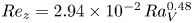$Re_z=2.94 \times 10^{-2}\,Ra_V^{0.48}$ ($\beta =0$), $Re_x=4.6 \times 10^{-3}\,Ra_V^{0.56}$ ($\beta =1.5^{\circ }$) and $Re_z=2.49 \times 10^{-2}vRa_V^{0.49}$ ($\beta =1.5^{\circ }$), respectively.

Another interpretation of the role of cell tilting in the formation of LSC suggests that the symmetry of the system is broken by the tilting of the cell, while there are two types of tilt: one is the tilt of the cell from the right, the other is the tilt of the cell from the left. When the cell is level, the buoyancy force is normal to the surface of the bottom plate, while when the cell is tilted from the right/left, the buoyancy force is no longer normal to the bottom plate: a component horizontal to the surface of the bottom plate (pointing to the right/left) emerges from the decomposition of the buoyancy force (as discussed in Zhang et al. Reference Zhang, Ding and Xia2021). This horizontal component of the buoyancy force induces horizontal component velocity in the right/left direction, thus facilitating the appearance of the LSC in the anticlockwise/clockwise direction. The one-to-one correspondence between the side of the tilt (right or left) and the direction of the LSC (anticlockwise or clockwise) implies that the causality is the following. The tilt of the cell breaks the symmetry, inducing horizontal buoyancy (the direction of the horizontal buoyancy depends on whether the cell is tilted from the right or the left side). Then this horizontal buoyancy induces horizontal velocity/motion,and after that, this horizontal velocity facilities the appearance of the LSC. In this sense, the horizontal velocity is a consequence of the symmetry breaking, but the horizontal velocity is the cause of the appearance of the LSC. It is worth mentioning that it was shown previously that the horizontal motion/velocity is crucial for the appearance of the LSC (Xi et al. Reference Xi, Lam and Xia2004).