


1. Introduction
The cavity is a typical configuration that is widely used in engineering applications. The high-speed flow past the open cavity will generate many complex vortices. The resulting intense flow will cause self-sustained pressure oscillations that damage the nearby components (Rossiter Reference Rossiter1964; Dix & Bauer Reference Dix and Bauer2000; Morton Reference Morton2007), and can also affect the fuel mixing and flame holding in the engine (Yeom, Seo & Sung Reference Yeom, Seo and Sung2013). Clear recognition of the flow structures underlying cavity flow oscillations will facilitate the development of effective flow control techniques.
The type of cavity flow is mainly related to two parameters. One is the length (L)-to-depth (D) ratio of the cavity, and the other is the Mach number of the free stream (Lawson & Barakos Reference Lawson and Barakos2011). At very low incoming velocity, three-dimensional instability modes of low Reynolds number open cavity flows are discussed by Meseguer-Garrido et al. (Reference Meseguer-Garrido, de Vicente, Valero and Theofilis2014), Citro et al. (Reference Citro, Giannetti, Brandt and Luchini2015) and Picella et al. (Reference Picella, Loiseau, Lusseyran, Robinet, Cherubini and Pastur2018). When the cavity is deep ( $L/D<6\sim 8$ for subsonic or $L/D <10$ for supersonic), the flow is regarded as ‘open’. The shear layer at the cavity mouth bridges the cavity. For shallow cavities ( $L/D >13$), the flow is considered to be ‘closed’. For this type, the shear layer expands over the cavity leading edge and impinges on the cavity floor (Stallings & Wilcox Reference Stallings and Wilcox1987; Plentovich, Stallings & Tracy Reference Plentovich, Stallings and Tracy1993). Between the ‘open’ and the ‘closed’ type is the transitional flow. The width (W) of the cavity also affects the characteristics of the cavity flow. The flow of the deep cavity is usually the ‘open’ type when $W/D$ is in the range of 1 to 8 (Plentovich et al. Reference Plentovich, Stallings and Tracy1993). Due to the rich physical phenomena and engineering applications, there is plenty of literature on the–topic of the ‘open’-type flow (Rowley & Williams Reference Rowley and Williams2006; Gloerfelt, Bogey & Bailly Reference Gloerfelt, Bogey and Bailly2007; Lawson & Barakos Reference Lawson and Barakos2011). In this type, the flow oscillations are driven by the mechanism of flow/acoustic resonance and form a self-sustained feedback loop (Rossiter Reference Rossiter1964). The frequencies of these resonances are well predicted by a semi-empirical formula proposed by Rossiter (Reference Rossiter1964), which is extended to the case of high Mach numbers by Heller & Bliss (Reference Heller and Bliss1975). While most research mainly focused on the spectral features of the pressure signals, less attention was paid to the detailed vortical structure characteristics in the cavity (Beresh, Wagner & Casper Reference Beresh, Wagner and Casper2016).
Through experimental measurements, a few papers considered the flow topology in a three-dimensional cavity. Crook, Lau & Kelso (Reference Crook, Lau and Kelso2013) conducted experiments on low-speed incompressible cavity flow in air and water. They provided a comprehensive description of the vortical structures in a cavity based on the velocity field obtained by particle image velocimetry. According to the study by Crook et al. (Reference Crook, Lau and Kelso2013), the front and rear, streamwise, small rear corner and recirculation vortices are symmetric about the cavity central plane, while the tornado-like vortex appears to be the primary indication of asymmetry within the cavity flow. The tornado-like vortex presents a stable focus in the velocity field of the bottom wall surface. The tornado-like vortex is so called because of the appearance of similarity to tornadoes generated under special meteorological conditions (Rotunno Reference Rotunno2013). A single tornado-like vortex is observed located near the cavity centreline at the front of the cavity, and the evidence of a second weak tornado-like vortex of opposite rotational direction can also be observed in the section not far from the bottom wall (Crook et al. Reference Crook, Lau and Kelso2013).
For high-speed three-dimensional cavity flow with sidewalls, velocimetry data are very rare due to the high requirements of experimental equipment and the difficulty of measurement (Beresh et al. Reference Beresh, Wagner and Casper2016). Different from the wall-free case, where the camera can be placed on the side to get the whole cross-sectional flow field directly, it is difficult to obtain velocity data near the front wall, back wall and the bottom of the cavity because of the large angle deviation from the cameras. The oil-flow visualization technique or numerical simulation is helpful to obtain the velocity field on the wall surface of the cavity. Atvars et al. (Reference Atvars, Knowles, Ritchie and Lawson2009) performed numerical and experimental studies on the cavity flow at Mach number 0.85. The flow visualization of the bottom wall surface shows that there are two tornado-like vortices upstream of the cavity. Dolling, Perng & Leu (Reference Dolling, Perng and Leu1997) carried out hypersonic experiments of cavity flow with Mach number 5 using the kerosene-diesel-lampblack oil-flow method. The flow patterns on the wall surface show that there is a pair of tornado-like vortices on the front floor. These two tornado vortices occupy almost 50 % of the cavity floor when a store is placed in the cavity. The fluorescence-oil-flow visualization technique uses light with a specific wavelength and energy to irradiate the oil pigment, which can better reveal the details of wall flow structures (Woodiga & Liu Reference Woodiga and Liu2009; Chen et al. Reference Chen, Zhu, Xu and Jiang2017). Using this visualization technique, Yang et al. (Reference Yang, Liu, Wang, Shi, Zhou and Zheng2018) studied the streamline pattern on the cavity surface for four different Mach numbers 0.6, 0.9, 1.5 and 2.0. A pair of stable foci that represents the tornado-like vortices can be observed in these four cases. In these high-speed three-dimensional cavity flows (Dolling et al. Reference Dolling, Perng and Leu1997; Atvars et al. Reference Atvars, Knowles, Ritchie and Lawson2009; Yang et al. Reference Yang, Liu, Wang, Shi, Zhou and Zheng2018), the rotational direction of the tornado-like vortices is opposite to that of the low-speed incompressible case. However, although the primary characteristics of the tornado-like vortices on the bottom wall surface are obtained, the time-averaged streamlines may mask the evolution characteristics of the tornado-like vortices. Moreover, a single cross-sectional plane of the streamline pattern near the bottom wall surface is insufficient to reveal the spatial structure of the whole vortex, leaving the structural properties of tornado-like vortices in high-speed cavity flows still unknown.
The research on the structure of the tornado-like vortex is to some extent driven by tornado phenomenology and climatology (Rotunno Reference Rotunno2013). Due to the measurement difficulty of the real tornado, the tornado-like vortex is produced by a special experimental facility in the laboratory to investigate its structure and movement (Rotunno Reference Rotunno2013; Refan & Hangan Reference Refan and Hangan2016, Reference Refan and Hangan2018; Ashrafi et al. Reference Ashrafi, Romanic, Kassab, Hangan and Ezami2021). The fluids converge towards the central axis along the bottom wall surface and turn upward, resulting in the generation of a strong axial flow, which is a typical swirling flow. The vortices in swirling flow have been studied extensively under the vortex breakdown phenomenon (Sarpkaya Reference Sarpkaya1971a,Reference Sarpkayab; Hall Reference Hall1972; Leibovich Reference Leibovich1978, Reference Leibovich1984; Lugt Reference Lugt1989). There are two major types of vortex breakdown, one is the spiral type (S-type), and another is called the bubble type (B-type) (Leibovich Reference Leibovich1978, Reference Leibovich1984). For the S-type, the vortex axis streamlines quickly deviate from the original direction with the development of the swirling flow. For the B-type, there is a conical core in the breakdown region, which is considered to be axisymmetric (Leibovich Reference Leibovich1984). The S-type and B-type can be observed simultaneously in some flows, e.g. on the lee sides of a delta wing (Lambourne & Bryer Reference Lambourne and Bryer1962). The theories that include the hydrodynamic instabilities, analogy to boundary layer separation (Hall Reference Hall1961, Reference Hall1972) and the concept of a critical state (Benjamin Reference Benjamin1962; Bossel Reference Bossel1969) were established to estimate the position of the vortex losing its stability (Lessen, Singh & Paillet Reference Lessen, Singh and Paillet1974; Nolan Reference Nolan2012), which lacks information on the detailed topology structures of the swirling vortex nevertheless.
To study the flow structure in the breakdown region, critical-point concepts have been applied in this area (Délery Reference Délery1994, Reference Délery2001), initially introduced by Legendre (Reference Legendre1956, Reference Legendre1977) for the original purpose of revealing the separation in three-dimensional flow. Perry & Chong (Reference Perry and Chong1987) provided a framework and methodology using the critical-point concepts to describe the flow patterns and gave a distribution of the critical points and their type. Chong, Perry & Cantwell (Reference Chong, Perry and Cantwell1990) further extend the theory to general three-dimensional flow fields. Based on the physical perspective of the vortex axis, Zhang (Reference Zhang1995) analysed the topological structure of an ideal steady vortex using the critical-point theory of ordinary differential equations. He gave a key parameter to determine the vortex structure in the cross-section perpendicular to the vortex axis and found an essential difference in the streamline pattern between the supersonic vortex and the subsonic vortex. The theory was extended to the unsteady state by Zhang, Zhang & Shu (Reference Zhang, Zhang and Shu2009) to study the topological structure of the unsteady vortex breakdown in the interaction between a normal shock wave and a longitudinal vortex. These authors found a quadru-helix structure in the tail of the vortex breakdown. Further, Zhang (Reference Zhang2018) found that there are tornado-like vortices in the separation surface of the three-dimensional flow over a prolate spheroid.
However, vast numerical simulation and experimental results indicate that the flow within the cavity with high-speed inflow is highly unsteady (Gloerfelt et al. Reference Gloerfelt, Bogey and Bailly2007; Lawson & Barakos Reference Lawson and Barakos2011). As a result, the tornado-like vortices in the cavity flow are different from the ideal spiral vortex and may have different spatial structures. The purpose of this paper is to study both the spatial structure and time evolution of tornado-like vortices in high-speed cavity flow. Based on the physical perspective of the vortex axis and the physical assumption of the swirling flow, the spatial structure of a tornado-like vortex can be revealed. We perform the numerical simulations of the cavity flow for Mach numbers 0.9 and 1.5, which are the typical Mach numbers in the range of high subsonic to supersonic speeds with important application backgrounds (Beresh et al. Reference Beresh, Wagner, Henfling, Spillers and Pruett2015a,Reference Beresh, Wagner, Pruett, Henfling and Spillersb). The geometry ratio of the cavity is  $L:W:D = 6:2:1$, which belongs to the open cavity flow (Stallings & Wilcox Reference Stallings and Wilcox1987; Plentovich et al. Reference Plentovich, Stallings and Tracy1993; Lawson & Barakos Reference Lawson and Barakos2011). We investigate the structural characteristics of the tornado-like vortices in the cavity using the critical point theory.
This paper is organized as follows. In § 2, we generalize the topological theory in the rectangular coordinate system to the curvilinear coordinate system. The sectional streamline pattern in the cross-section perpendicular to the vortex axis and the meridional plane, and the relations between the critical point in the meridional plane and the streamline pattern in the cross-sectional plane perpendicular to the vortex axis are analysed. In § 3, we present the numerical method and computational conditions for solving the Navier–Stokes equations in three-dimensional cavity flow and the validation of numerical results. In § 4, based on the topological analysis and numerical simulation, the evolution and the spatial of the tornado-like vortices in the cavity flow are analysed. Section 5 contains our conclusion.
2. Topological analysis of spiral vortex
2.1. In the cross-section perpendicular to the vortex axis
In cavity flow, the spiral feature of the tornado-like vortex is very complex. According to the study by Crook et al. (Reference Crook, Lau and Kelso2013), its spiral features vary along its axis. In this section, the topology method (Zhang Reference Zhang1995; Zhang et al. Reference Zhang, Zhang and Shu2009) is used to analyse the spiral characteristic of the tornado-like vortex in the cavity. In the analytical studies of Zhang (Reference Zhang1995) and Zhang et al. (Reference Zhang, Zhang and Shu2009), an effective formula is provided to determine the streamline pattern of a swirling flow on the cross-section perpendicular to the vortex axis. The formula is obtained based on the assumption that the vortex axis is a straight line. However, the vortex axis is usually in a curve shape in real flows. Here, we first generalize the topology theory to the case of the curvilinear vortex axis. The deduction is based on an orthogonal curvilinear coordinate system  $(q_1, q_2, q_3)$, as shown in figure 1. Here, $u_1$, $u_2$ and $u_3$ are the velocity components corresponding to the directions of $q_1$, $q_2$ and $q_3$, respectively. Without loss of generality, we set the vortex axis in the axis $q_1$ direction.

Figure 1. Schematic diagram of curvilinear coordinate system.
The continuity equation of the flow in this curvilinear coordinate system is
 \begin{equation} \frac{\partial \rho}{\partial t} + \frac{1}{H_1 H_2 H_3} \left( \frac{\partial(\rho H_2 H_3 u_1)}{\partial q_1} + \frac{\partial(\rho H_3 H_1 u_2)}{\partial q_2}+ \frac{\partial(\rho H_1 H_2 u_3)}{\partial q_3} \right) = 0, \end{equation}
where  $H_1$, $H_2$ and $H_3$ are the Lame coefficients, $\rho$ is the density of the fluids and $t$ represents the time. Their expressions are
 \begin{equation} H_i = \sqrt{\left( \frac{\partial x}{\partial q_i} \right)^2 + \left( \frac{\partial y}{\partial q_i} \right)^2 + \left( \frac{\partial z}{\partial q_i} \right)^2},\quad i=1,2,3, \end{equation}
where  $x$,
$x$,  $y$ and $z$ are the axes of the normal orthogonal coordinate system. The momentum equation in the direction of $q_1$ is
 \begin{align} \frac{\mathrm{D} u_{1}}{\mathrm{D} t}+\frac{u_{1} u_{2}}{H_{1} H_{2}} \frac{\partial H_{1}}{\partial q_{2}}+\frac{u_{1} u_{3}}{H_{1} H_{3}} \frac{\partial H_{1}}{\partial q_{3}}-\frac{u_{2}^{2}}{H_{1} H_{2}} \frac{\partial H_{2}}{\partial q_{1}}-\frac{u_{3}^{2}}{H_{3} H_{1}} \frac{\partial H_{3}}{\partial q_{1}} ={-}\frac{1}{H_{1} \rho}\frac{\partial p}{\partial q_{1}}+\frac{\tau_\mu}{Re}. \end{align}
Here,  $\mathrm {D}/\mathrm {D} t$ is the material derivative and $p$ is the pressure. The last term $\tau _\mu /Re$ is related to the viscosity, $\tau_\mu$ is a function of dynamic viscous coefficient $\mu$ and velocities, Re is the Reynolds number. For inviscid flow or high Reynolds number flow ( $Re\gg 1$), this term is infinitesimal and can be neglected.
Because the vortex axis is a streamline, the boundary condition on the vortex axis is
 \begin{equation} u_2(q_1) = u_3(q_1) = 0. \end{equation}
Along the vortex axis of  $q_1$, (2.3) can be simplified as:
 \begin{equation} \frac{\partial u_{1}}{\partial t} + \frac{u_1}{H_1} \frac{\partial u_{1}}{\partial q_1}={-}\frac{1}{H_{1} \rho}\frac{\partial p}{\partial q_{1}}. \end{equation}
The velocity in the near region of the vortex axis can be expressed by a Taylor expansion
 \begin{equation}
\left.\begin{gathered} u_1(q_1,q_2,q_3)= u_1^1 +
\frac{\partial u_1}{\partial q_1}q_1 + \frac{\partial
u_1}{\partial q_2}q_2 + \frac{\partial u_1}{\partial
q_3}q_3 + O(q_1^2,q_2^2,q_3^2), \\ u_2(q_2,q_3) =
\frac{\partial u_2}{\partial q_2}q_2 + \frac{\partial
u_2}{\partial q_3}q_3 + O(q_2^2,q_3^2),\\ u_3(q_2,q_3) =
\frac{\partial u_3}{\partial q_2}q_2 + \frac{\partial
u_3}{\partial q_3}q_3 + O(q_2^2,q_3^2).
\end{gathered}\right\}
\end{equation}
\begin{equation}
\left.\begin{gathered} u_1(q_1,q_2,q_3)= u_1^1 +
\frac{\partial u_1}{\partial q_1}q_1 + \frac{\partial
u_1}{\partial q_2}q_2 + \frac{\partial u_1}{\partial
q_3}q_3 + O(q_1^2,q_2^2,q_3^2), \\ u_2(q_2,q_3) =
\frac{\partial u_2}{\partial q_2}q_2 + \frac{\partial
u_2}{\partial q_3}q_3 + O(q_2^2,q_3^2),\\ u_3(q_2,q_3) =
\frac{\partial u_3}{\partial q_2}q_2 + \frac{\partial
u_3}{\partial q_3}q_3 + O(q_2^2,q_3^2).
\end{gathered}\right\}
\end{equation}
Here,  $u_1^1$ is velocity component along the axis $q_1$ at the origin of the coordinate system. The variables $u_2^1$, $u_3^1$, $\partial u_2 / \partial q_1$ and $\partial u_3 / \partial q_1$ vanish in (2.6) because $u_2$ and $u_3$ are constant and equal to zero along the axis of $q_1$ according to (2.4).
The streamlines of the vortex are defined by
 \begin{equation} \frac{\mathrm{d} \boldsymbol{X}}{\mathrm{d} t}=\boldsymbol{U}, \end{equation}
where  $\boldsymbol {X}=(q_1,q_2,q_3)$ is the space position, and $\boldsymbol {U}=(u_1,u_2,u_3)$ is the vector of the velocity. The local velocity field around a point $\boldsymbol {X}_0$ can be expressed to the first order as
 \begin{equation} \boldsymbol{U}(\boldsymbol{X}+\delta \boldsymbol{X})=\boldsymbol{U}(\boldsymbol{X})+ \boldsymbol{\mathsf{D}} \delta\boldsymbol{X}+O(\|\delta \boldsymbol{X}\|^2), \end{equation}
where  $\boldsymbol{\mathsf{D}}=\nabla \boldsymbol {U}$ is the velocity gradient tensor. According to the vortex definition proposed by Chong et al. (Reference Chong, Perry and Cantwell1990), matrix $\boldsymbol{\mathsf{D}}$ has complex eigenvalues in the vortex core region. Thus, for the swirling flow, matrix $\boldsymbol{\mathsf{D}}$ can be transformed into a canonical form matrix $\boldsymbol{\mathsf{A}}'$ (Chong et al. Reference Chong, Perry and Cantwell1990; Zhou et al. Reference Zhou, Adrian, Balachandar and Kendall1999)
 \begin{align}
\boldsymbol{\mathsf{D}}&=(\boldsymbol{v}_{r}, \boldsymbol{v}_{c r},
\boldsymbol{v}_{c i})\ {\cdot}\ \left(\begin{array}{@{}ccc@{}}
\lambda_{r} & & \\ & \lambda_{c r} & \lambda_{c i} \\ &
-\lambda_{c i} & \lambda_{c r}
\end{array}\right)\ {\cdot}\ (\boldsymbol{v}_{r},
\boldsymbol{v}_{c r}, \boldsymbol{v}_{c i})^{{-}1}
\nonumber\\ &= (\boldsymbol{v}_{r}, \boldsymbol{v}_{c r},
\boldsymbol{v}_{c i})\ {\cdot}\ \boldsymbol{\mathsf{A}}' \ {\cdot}\
(\boldsymbol{v}_{r}, \boldsymbol{v}_{c r},
\boldsymbol{v}_{c i})^{{-}1},
\end{align}
\begin{align}
\boldsymbol{\mathsf{D}}&=(\boldsymbol{v}_{r}, \boldsymbol{v}_{c r},
\boldsymbol{v}_{c i})\ {\cdot}\ \left(\begin{array}{@{}ccc@{}}
\lambda_{r} & & \\ & \lambda_{c r} & \lambda_{c i} \\ &
-\lambda_{c i} & \lambda_{c r}
\end{array}\right)\ {\cdot}\ (\boldsymbol{v}_{r},
\boldsymbol{v}_{c r}, \boldsymbol{v}_{c i})^{{-}1}
\nonumber\\ &= (\boldsymbol{v}_{r}, \boldsymbol{v}_{c r},
\boldsymbol{v}_{c i})\ {\cdot}\ \boldsymbol{\mathsf{A}}' \ {\cdot}\
(\boldsymbol{v}_{r}, \boldsymbol{v}_{c r},
\boldsymbol{v}_{c i})^{{-}1},
\end{align}
where  $\boldsymbol{\mathsf{A}}'$ has a real eigenvalue $\lambda _r$ and a conjugate pair of complex eigenvalues $\lambda _{cr}\pm \lambda _{ci}\ {\cdot }\ \mathrm {i}$. The corresponding eigenvectors of these three eigenvalues are $\boldsymbol {v}_r$, $\boldsymbol {v}_{cr}$ and $\boldsymbol {v}_{ci}$. As discussed by Zhou et al. (Reference Zhou, Adrian, Balachandar and Kendall1999), the local flow is either stretched or compressed along the axis $\boldsymbol {v}_r$. The particular sectional streamlines of interest lie in the cross-section spanned by the eigenvectors $\boldsymbol {v}_{cr}$ and $\boldsymbol {v}_{ci}$, on which the flow is swirling. As shown in figure 1, the vortex axis is denoted by the $q_1$-axis. Then, in the cross-section perpendicular to the vortex axis of $q_1$, the sectional streamline can be described by
 \begin{equation} \frac{\mathrm{d}q_3}{\mathrm{d}q_2} = \frac{u_3}{u_2}. \end{equation}
By substituting (2.6) into the above formula and neglecting the higher-order terms, we can get
 \begin{equation} \frac{\mathrm{d}q_3}{\mathrm{d}q_2} = \frac{u_3}{u_2} = \frac{\dfrac{\partial u_3}{\partial q_2}q_2 + \dfrac{\partial u_3}{\partial q_3}q_3}{\dfrac{\partial u_2}{\partial q_2}q_2 + \dfrac{\partial u_2}{\partial q_3}q_3}. \end{equation}
 According to the critical-point theory of ordinary differential equations (Jordan & Smith Reference Jordan and Smith1977), the sectional streamline pattern in the neighbourhood of the vortex axis is related to the discriminant of the eigenvalue equation of the rate-of-deformation tensor matrix  $\boldsymbol{\mathsf{F}}=\partial (u_2,u_3) / \partial (q_2, q_3)$ in the cross-sectional plane. The discriminant depends on the opposite of the trace and determinant of matrix $\boldsymbol{\mathsf{F}}$ as follows:
 \begin{equation} R={-}\left(\frac{\partial u_2}{\partial q_2} + \frac{\partial u_3}{\partial q_3}\right), \quad q=\frac{\partial u_2}{\partial q_2}\frac{\partial u_3}{\partial q_3} - \frac{\partial u_3}{\partial q_2}\frac{\partial u_2}{\partial q_3}, \end{equation}
where  $R$ and $q$ are the coefficients of the first and zero orders of the eigenvalue equation of matrix $\boldsymbol{\mathsf{F}}$. The critical points in a two-dimensional space include the focus, node and saddle. The classification of the critical points related to these two variables $R$ and $q$ is replotted following Perry & Chong (Reference Perry and Chong1987) and Délery (Reference Délery2001), as shown in figure 2. For a swirling flow, the streamline pattern in the cross-sectional plane perpendicular to the vortex axis is related to the region above the parabolic curve $q=R^2/4$, as shown in figure 2. In the first quadrant, the streamline pattern appears as a stable focus. In the second quadrant, the streamline pattern appears as an unstable focus. Therefore, the spiral direction is determined by the positive and negative signs of function
 \begin{equation} \lambda(q_1,t) = R ={-}\left(\frac{\partial u_2}{\partial q_2} + \frac{\partial u_3}{\partial q_3}\right). \end{equation}
The details can be found in Chong et al. (Reference Chong, Perry and Cantwell1990) and Zhang et al. (Reference Zhang, Zhang and Shu2009). If  $\lambda >0$, the sectional streamlines spiral inward in the cross-section perpendicular to the vortex axis. If $\lambda <0$, the sectional streamlines in this cross-section spiral outward. If $\lambda$ changes sign along the vortex axis, one more limit cycle may appear in the sectional streamline pattern (Jordan & Smith Reference Jordan and Smith1977; Zhang et al. Reference Zhang, Zhang and Shu2009). By substituting the continuity equation (2.1) and the boundary condition (2.4), the function $\lambda$ is
 \begin{equation} \lambda(q_1,t) = \frac{H_2}{\rho}\frac{\partial \rho}{\partial t}+ \frac{1}{\rho H_1 H_3} \frac{\partial (\rho H_2 H_3 u_1)}{\partial q_1} + \left(\frac{H_2}{H_3} - 1\right) \frac{\partial u_3}{\partial q_3}. \end{equation}
Figure 2. The classification of critical points.
For steady flow, the first term on the right side of (2.14) vanishes, and the function  $\lambda$ is
 \begin{equation} \lambda(q_1) = \frac{H_2}{ H_1} \frac{u_1}{\rho} \frac{\partial \rho}{\partial q_1} + \frac{H_2}{H_1} \frac{\partial u_1}{\partial q_1} + \frac{u_1}{H_1 H_3} \frac{\partial(H_2 H_3)}{\partial q_1} + \left(\frac{H_2}{H_3} - 1\right) \frac{\partial u_3}{\partial q_3}. \end{equation}
 If the flow is isentropic,  $\partial p/\partial \rho = a^2$. Here, $a$ is the local sound speed. By substituting the Euler equation (2.5), we can obtain the function $\lambda$ along the vortex axis of $q_1$
$q_1$
 \begin{equation} \lambda(q_1) = \frac{H_2}{ H_1} \frac{1}{\rho u_1} (M_1^2 - 1) \frac{\partial p}{\partial q_1} + \frac{u_1}{H_1 H_3} \frac{\partial(H_2 H_3)}{\partial q_1} + \left(\frac{H_2}{H_3} - 1\right) \frac{\partial u_3}{\partial q_3}, \end{equation}
where  $M_1$ is the local Mach number on the vortex axis.
If the vortex axis is a straight line, the orthogonal curvilinear coordinate system  $(q_1, q_2, q_3)$ degenerates into the normal orthogonal coordinate system $(x, y, z)$, then we have $H_1=H_2=H_3=1$. In this case, the function $\lambda (q_1)$ will degenerate into the form $1/(\rho u_1)(M_1^2 - 1)\partial p/\partial q_1$ (Zhang Reference Zhang1995; Zhang et al. Reference Zhang, Zhang and Shu2009), which shows that there is an essential difference between a subsonic vortex and a supersonic vortex.
2.2. In the meridional plane
In the meridional plane passing through the vortex axis of  $q_1$, without loss of generality, the $q_1-q_3$ plane is set as the meridional plane, and the sectional streamline can be expressed by
 \begin{equation} \frac{\mathrm{d}q_3}{\mathrm{d}q_1} = \frac{u_3}{u_1}. \end{equation}
When  $u_1^1=0$, the corresponding position is a critical point. In the vicinity of the critical point, by applying (2.6) and neglecting the higher-order terms, we can get
 \begin{equation} \frac{\mathrm{d}q_3}{\mathrm{d}q_1} = \frac{\dfrac{\partial u_3}{\partial q_3}q_3}{\dfrac{\partial u_1}{\partial q_1}q_1 + \dfrac{\partial u_1}{\partial q_3}q_3}. \end{equation}
Similarly, the sectional streamline pattern in the vicinity of the critical point depends on the following two variables:
 \begin{equation} R={-}\left(\frac{\partial u_1}{\partial q_1} + \frac{\partial u_3}{\partial q_3}\right), \quad q(q_1,t)=\frac{\partial u_1}{\partial q_1}\frac{\partial u_3}{\partial q_3}. \end{equation}
 Through simple derivation, we have  $R^2-4q=(\partial u_1 / \partial q_1 - \partial u_3 / \partial q_3)^2 \geq 0$. Thus, the streamline pattern in the meridional plane is related to the region below the parabolic curve $q = R^2/4$, as shown in figure 2. The critical point is a node or saddle, depending on the sign of $q(q_1,t)$. If $q(q_1,t)>0$, the critical point is a node. If $q(q_1,t)<0$, the critical point is a saddle. The possible streamline pattern is shown in figure 3 (Zhang Reference Zhang2005; Zhang et al. Reference Zhang, Zhang and Shu2009).

Figure 3. Schematic diagram of the streamline pattern in the meridional plane.
2.3. Relations of streamline pattern between the meridional and perpendicular planes
Now we analyse the relations between the critical point in the meridional plane and the streamline pattern in the cross-sectional plane perpendicular to the vortex axis. For the first type of saddle, as shown in figure 3(a), the axial velocity  $u_1$ is zero. The axial velocity changes from positive to negative when it passes through this type of saddle, and thus we have $\partial u_1 / \partial q_1 < 0$. Since $q=\partial u_1 / \partial q_1 \times \partial u_3 /\partial q_3<0$ holds at the saddle, it must have $\partial u_3 / \partial q_3>0$. Based on the symmetry of the ideal swirling flow as assumed at the beginning of this section, the meridional plane can also be set at the $q_1-q_2$ plane. Thus, we also have $\partial u_2/ \partial q_2>0$. Putting these into (2.13), we have $\lambda <0$. According to the discussion in § 2.1, the streamlines spiral outward in the cross-sectional plane perpendicular to the axis at this type of saddle.
For the second type of saddle, as shown in figure 3(b), the change of the velocity component  $u_1$ along the vortex axis is opposite to that of the first type. Similarly, based on $q=\partial u_1 / \partial q_1 \times \partial u_3 / \partial q_3<0$ and the symmetry, we can get $\partial u_3 / \partial q_3<0$ and $\partial u_2 / \partial q_2<0$. Putting these into (2.13), we have $\lambda >0$. Therefore, the streamlines spiral inward in the cross-sectional plane perpendicular to the axis at this type of saddle.
If the critical point is a node, as shown in figure 3(c),  $u_1$ changes from negative to positive as the axis passes through it, and thus we have $\partial u_1 / \partial q_1 > 0$. Since $q=\partial u_1 / \partial q_1 \times \partial u_3 / \partial q_3>0$ holds at the node, it must have $\partial u_3 / \partial q_3>0$. If the flow is steady, $\partial \rho / \partial t = 0$. The continuity equation (2.1) can be written as
 \begin{equation} \frac{\partial(\rho H_2 H_3 u_1)}{\partial q_1} + \frac{\partial(\rho H_3 H_1 u_2)}{\partial q_2}+ \frac{\partial(\rho H_1 H_2 u_3)}{\partial q_3} = 0. \end{equation}
At a critical point,  $u_1=0$, combined with the axial velocity condition in (2.4), the above equation can be simplified as
 \begin{equation} H_2 H_3 \frac{\partial u_1}{\partial q_1} + H_3 H_1\frac{\partial u_2}{\partial q_2}+ H_1 H_2 \frac{\partial u_3}{\partial q_3} = 0. \end{equation}
Combined with this equation, (2.13) can be written as
 \begin{equation} \lambda(q_1)= \frac{H_2}{H_1}\frac{\partial u_1}{\partial q_1} + \left(\frac{H_2}{H_3} - 1 \right)\frac{\partial u_3}{\partial q_3}. \end{equation}
As discussed above, the first term of the right-hand side of the above equation is positive.
To determine the sign of the function  $\lambda$, we now estimate the coefficient of the second term of the right-hand side in (2.22). Without loss of generality, the origin of the coordinate system is set at the critical point. Let $\theta _{2,Y}$ denote the angle between the curvilinear axis $q_2$ and perpendicular projection in the $X$–
$X$– $Z$ plane, as shown in figure 4. Similarly, we have the notation $\theta _{2,X}$, $\theta _{2,Z}$, $\theta _{3,X}$, $\theta _{3,Y}$, $\theta _{3,Z}$. For a small $\Delta q_2$, we have $\Delta y = \Delta q_2 \times \sin \theta _{2,Y}$. Thus, the partial derivative can be approximately calculated by $\partial y / \partial q_2 = \sin \theta _{2,Y}$. Similarly, we could calculate all the partial derivatives in (2.2). Putting all these results into (2.2), we can get
 \begin{equation} \frac{H_2}{H_3}-1 = \sqrt{\frac{\sin^2 \theta_{2,X}+\sin^2 \theta_{2,Y}+\sin^2 \theta_{2,Z}} {\sin^2 \theta_{3,X}+\sin^2 \theta_{3,Y}+\sin^2 \theta_{3,Z}}}-1. \end{equation}
If the curvature of the vortex axis is small, the variables  $\theta _{2,X}$, $\pi /2-\theta _{2,Y}$, $\theta _{2,Z}$, $\theta _{3,X}$, $\theta _{3,Y}$, $\pi /2-\theta _{3,Z}$ are small. Let $\epsilon$ denote the smallest of these variables. If we have $\epsilon \sim o(1)$, (2.23) can be expanded on $\epsilon$ by a Taylor expansion, to give
 \begin{equation} \frac{H_2}{H_3}-1 \sim O(\epsilon^2) \sim o(\epsilon) \ll 1. \end{equation}
That is, the coefficient of the second term of the right-hand side in (2.22) is smaller than  $\epsilon$. Thus, the sign of function $\lambda$ depends on the first term and is positive in this case. If the two coordinate systems coincide, (2.22) degenerates as $\lambda = \partial u_1 / \partial q_1 > 0$. Therefore, according to the discussion above, the streamlines spiral inward in the cross-sectional plane perpendicular to the axis at this type of node.

Figure 4. Schematic diagram of the two coordinate systems.
Now we analyse the relationship between the property of the function  $\lambda (q_1,t)$ and the B-type or S-type breakdown. For the S-type, the vortex axis streamlines quickly deviate from the original direction (Zhang Reference Zhang1995). For the B-type, there are two critical points in the streamline pattern of the meridional plane, as shown in figure 3(c). As a result, the property of the function $\lambda (q_1,t)$, especially the sign changes along the vortex axis, are different. Based on the discussion above in this section, a criterion of the function $\lambda (q_1,t)$ for the B-type or S-type breakdowns is as follows: in the initial and breakdown region of a swirling vortex, for the B-type, there is $q_1^1 < q_1^2 < q_1^3 < q_1^4$ ( $q_1^{1}$, $q_1^{2}$, $q_1^{3}$ and $q_1^{4}$ are four points along the vortex axis), such that $\lambda (q_1^1,t)>0$, $\lambda (q_1^2,t)<0$, $\lambda (q_1^3,t)>0$ and $\lambda (q_1^4,t)<0$, that is, the function $\lambda (q_1,t)$ has and only has three zero points and its initial value is greater than zero; for the S-type, there is $q_1^1 < q_1^2$, such that $\lambda (q_1^1,t)>0$, $\lambda (q_1^2,t)<0$, and for any $q_1^3 > q_1^2$, it has $\lambda (q_1^3,t)<0$, that is, the function $\lambda (q_1,t)$ has and only has one zero point and its initial value is greater than zero.
From (2.21), we can simply get another inference. Since  $\partial u_1 / \partial q_1 > 0$ and $\partial u_3 / \partial q_3 > 0$ hold at the node in the meridional plane of $q_1-q_3$, substituting these into (2.21), we have $\partial u_2 / \partial q_2 < 0$. This leads to $\tilde {q}=\partial u_1 / \partial q_1 \times \partial u_2 / \partial q_2 < 0$. Similar to the analysis in § 2.2, the critical-point type in the meridional plane of $q_1-q_2$ is a saddle. The corollary is, if the type of critical point in the meridional plane is a node, then, in another meridional plane perpendicular to this meridional plane, the critical point is a saddle. That is, the streamline pattern is non-axisymmetric about the vortex axis at this critical point. This inference is not strange, because if the streamline pattern is axisymmetric at the node, the ‘source’ of the fluids in all directions in the vicinity of the critical point is the critical point itself, which is contradictory with the fact that the fluids cannot spontaneously materialize.
3. Numerical simulation
3.1. Governing equations
The three-dimensional unsteady compressible Navier–Stokes equations without external forces are solved numerically. By introducing the tensor notations, the conservative form of the non-dimensional Navier–Stokes equations can be written as follows:
 $$\begin{gather} {\partial_t}\rho + {\partial_j}(\rho {u_j}) = 0, \end{gather}$$
 $$\begin{gather}{\partial_t}(\rho {u_j}) + {\partial_i}(\rho {u_i}{u_j} + p{\delta_{ij}}) = \frac{1}{Re}{\partial_i}{\sigma_{ij}}, \end{gather}$$
 $$\begin{gather}{\partial_t}E + {\partial_i}\left( {{u_i}(E + p)} \right) = \frac{1}{Re}{\partial_i}({\sigma _{ij}}{u_j} - \dot{q}_i), \end{gather}$$
where  $u_i = (u, v, w)$, $\rho$, $p$ and $E$ are the velocity components, the density, the pressure and the total energy, respectively. $\delta_{ij}$ is a Kronecker operator.
The total energy  $E$ is expressed by
 \begin{equation} E = \frac{p}{{\gamma - 1}} + \frac{1}{2}\rho {u_i}{u_i}. \end{equation}
Here,  $\sigma _{ij}$ is the viscous stress term, under the assumption of Newtonian fluid it can be written as
 \begin{equation} {\sigma_{ij}} = \mu ({u_{ij}} + {u_{ji}}) - \tfrac{2}{3}\mu \partial_k u_k \delta_{ij}. \end{equation}
Also,  $q$ is the heat flux ratio and is a function of the temperature $T_m$
$T_m$
 \begin{equation} \dot{q}_i ={-} \frac{1}{{( {\gamma - 1} ){Ma^2}}} \left(\frac{\mu_l}{Pr_l} + \frac{\mu_t}{Pr_t}\right){\partial_i}T_m, \end{equation}
where  $Pr_l=0.7$ and $Pr_t=0.9$ are the laminar and turbulent Prandtl numbers, respectively.
The dynamic viscous coefficient  $\mu = \mu _l + \mu _t$, where $\mu _l$ and $\mu _t$ are the laminar and turbulent dynamic viscous coefficient, respectively. The laminar dynamic viscous coefficient $\mu _l$ is calculated by Sutherland's formula
 \begin{equation} \mu_l = T_m^{3/2}\frac{{1 + C}}{{T_m + C}}, \quad C = \frac{{110.4\ {\rm K}}}{{T_\infty ^*}}. \end{equation}
The turbulent dynamic viscous coefficient  $\mu _t$ is calculated by the Spalart–Allmaras (SA) turbulence model (Spalart & Allmaras Reference Spalart and Allmaras1994) and delayed-detached-eddy simulation (DDES) method (Shur et al. Reference Shur, Spalart, Strelets and Travin2008).
The fluid is assumed to be an ideal gas, and thus satisfies
 \begin{equation} p = \frac{\rho T_m}{\gamma \,Ma^2}. \end{equation}
Finally, the Mach number  $Ma$ and the Reynolds number $Re$ are constants related to specific computational cases. The ratio of specific heat is set as $\gamma = 1.4$.
3.2. Numerical method and flow configuration
In this paper, the cavity size is set according to the experimental model designed by the High Speed Aerodynamics Research Institute of China Aerodynamics Research and Development Center (CARDC) (Yang et al. Reference Yang, Liu, Wang, Shi, Zhou and Zheng2018). The length, width and depth of the cavity are  $L=200$ mm, $W =66.67$ mm and $D=33.33$ mm, respectively ( $L:W:D=6:2:1$). A schematic diagram of the cavity configuration is shown in figure 5. The origin of the coordinate system is located at the corner of the leading edge of the cavity. The $X$-axis, $Y$-axis and $Z$-axis are the transverse, longitudinal and spanwise directions, respectively. The ranges of the computational domain are $-16D\leq x \leq 20D$, $-1D \leq y \leq 12D$ and $-3-D \leq z \leq 5D$. The wall is assumed to be adiabatic.

Figure 5. Schematic diagram of the cavity configuration.
All variables are non-dimensionalized by the reference density  $\rho _\infty$, the reference temperature $T_\infty =288.15$ K, the cavity depth $D$ and the sound speed $a_\infty$, respectively. Here, the subscript $\infty$ represents the flow parameters at infinity. Table 1 shows the computational parameters for the two cases.
Table 1. The computational parameters for different cases (Reynold number  $Re$ is based on the length of the cavity).

The governing equations are solved numerically using a finite volume solver with the SA-DDES method (Shur et al. Reference Shur, Spalart, Strelets and Travin2008). The spatial convective flux is interpolated by a third-order weighted essentially non-oscillatory (WENO) method (Zhang, Jiang & Shu Reference Zhang, Jiang and Shu2008). The implicit lower–upper symmetric Gauss–Seidel (LU-SGS) method (Jameson & Yoon Reference Jameson and Yoon1987) is adopted for time discretization.
3.3. Validation
We undertook a grid convergence analysis for the Mach number 0.9 case with three meshes. A Cartesian stretched grid that is dense near the wall and sparse in the far-field region is used, as shown in figure 6. To resolve the boundary layer and the shear layer, the minimum grid spacing of the coarse, middle and fine grids near the wall is set as  $2.0\times 10^{-4}D$ and $1.0\times 10^{-4}D$ and $5.0\times 10^{-5}D$, respectively. The non-dimensional wall distance (Pope Reference Pope2000) for each mesh is approximately $y^+\approx 5.2$, 2.8, 1.3, respectively. The vertical grids above the cavity mouth are adjusted to capture the development of the shear layer. The number of grids is increased in all three directions $X$,
$X$,  $Y$ and $Z$. The total numbers of grid points of each mesh are 8 million, 11 million and 28 million, respectively. Figure 7 shows the time-averaged density and pressure of the central plane on the cavity floor. There are few differences in the density and the pressure between the middle grid case and the fine grid case. Therefore, the numerical results are approximately grid independent. Hereafter, the middle grid is used to compute the cavity flow. For the Mach number 1.5 case, since the Reynolds number is greater than the Mach number 0.9 case, the minimum grid spacing near the solid wall is adjusted to $6.0\times 10^{-6}D$ ( $y^+\approx 0.2$) based on the middle mesh to ensure simulation accuracy. The number of grid points is approximately 17 million.

Figure 6. A part of grid on the spanwise central plane.

Figure 7. Time-averaged density and pressure of the central plane on the cavity floor, the solid line (—–) refers to the middle grid case, the dashed dot dot line (– $\ {\cdot \cdot}\ $–, red) refers to the coarse grid case, the dashed line (– –, green) refers to the fine grid case.
Figure 8 shows the overall sound pressure level (OASPL) of the numerical results at different locations of the central plane in the cavity and their comparison with the experimental results (Yang et al. Reference Yang, Liu, Wang, Shi, Zhou and Zheng2018). For Mach numbers 0.9 and 1.5, the maximum differences of the OASPL between the computation and experiment are 1.62 and 2.59 dB respectively, and the averaged errors of the OASPL for different locations in the cavity are 0.74 and 1.22 dB, respectively. The present computational results are in good agreement with the experimental results.

Figure 8. Comparison between the experiments (Yang et al. Reference Yang, Liu, Wang, Shi, Zhou and Zheng2018) and the present numerical results of the OASPL at different locations in the cavity; (a)  $Ma=0.9$ and (b) $Ma=1.5$.
Figure 9 shows the spectra of the pressure perturbation signals of the present numerical results and experimental results (Yang et al. Reference Yang, Liu, Wang, Shi, Zhou and Zheng2018) at the front and back walls of the cavity for the two cases. The spectra represent the intensity of different frequencies of the oscillations in the cavity and are converted from the power spectral density (PSD) as follows:
 \begin{equation} \mathrm{SPL} = 10 \log_{10} \frac{\mathrm{PSD}}{P^2_{ref}}, \end{equation}
where  $P_{ref}=2\times 10^{-5}$ Pa is the reference pressure that represents the hearing threshold value of sound of 1 kHz. The PSD is computed using the Yule–Walker autoregressive method (Brockwell & Davis Reference Brockwell and Davis1991). It can be noted that the frequencies of the most energetic peaks in the spectra agree well with the experimental results.

Figure 9. The spectra of the pressure perturbation signals at the front (suffix ‘-F’,  $(x,y,z)=(0,-0.88,1)$) and back (suffix ‘-B’, $(x,y,z)=(6,-0.88,1)$) walls of the cavity for the two cases. Experimental results (Yang et al. Reference Yang, Liu, Wang, Shi, Zhou and Zheng2018): dash-dot line (- $\ {\cdot}\ $- $\ {\cdot}\ $); the present numerical results: solid line (—–); (a) $Ma=0.9$ and (b) $Ma=1.5$.
Figure 10 contains the time-averaged streamlines on the wall of the cavity based on the numerical results and their comparison with the experimental photographs (Zhou et al. Reference Zhou, Yang, Wang, Liu and Shi2018). The experimental figures are plotted using the coloured fluorescence-oil-flow technique, which allows us to reveal the detailed topological flow structures on the wall surface (Woodiga & Liu Reference Woodiga and Liu2009; Chen et al. Reference Chen, Zhu, Xu and Jiang2017). All the walls of the cavity are unfolded like a box for convenient comparison. It can be noted that the flow characteristics of the numerical results, such as the separation lines, the reattached lines and critical points engraved on each solid wall by the vortices motion, are qualitatively consistent with the experimental results.

Figure 10. Comparison of numerical time-averaged streamlines of the solid wall of the cavity with the coloured fluorescence-oil-flow photograph: (a, b) show the numerical time-averaged streamlines with pressure coefficient contours; (c, d) show the experimental results (Zhou et al. Reference Zhou, Yang, Wang, Liu and Shi2018); (a)  $Ma=0.9$, (b) $Ma=1.5$, (c) $Ma=0.9$ and (d) $Ma=1.5$.
4. Evolution of tornado-like vortex
As shown in figures 10(a) and 10(b), there is a pair of stable foci upstream of the bottom of the cavity, and their rotational directions are opposite. The similar streamline patterns of the tornado-like vortices of the present two cases can also be observed in the hypersonic experiments conducted by Dolling et al. (Reference Dolling, Perng and Leu1997). In the low-speed incompressible experiments performed by Crook et al. (Reference Crook, Lau and Kelso2013), the rotation directions of tornado-like vortices are opposite to the present two cases, which may be caused by the different impingement strength between the shear layer and back wall, resulting in different strengths of the reverse flow along the bottom wall and sidewalls. Although there is a slight difference between the experimental results and the numerical results, as shown in figure 10, it can be observed in experiments that the focus pair of tornado-like vortices is asymmetric about the central plane. This asymmetrical feature can also be observed in the experimental result of Dolling et al. (Reference Dolling, Perng and Leu1997). In the low-speed incompressible flow (Crook et al. Reference Crook, Lau and Kelso2013), the asymmetrical feature of the tornado-like vortices is more obvious. In this section, we try to reveal the evolution and spatial structures of the tornado-like vortices.
4.1. The case  $Ma=0.9$

4.1.1. Movement of the vortices
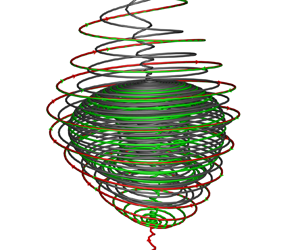
Figure 11 shows the instantaneous three-dimensional streamlines of the tornado-like vortices at different instants in two cycles of oscillation. For the present Mach number 0.9 case, the dominant mode is the second Rossiter mode (Rossiter Reference Rossiter1964) and its non-dimensional frequency is  $St_2=0.65$ (Yang et al. Reference Yang, Liu, Wang, Shi, Zhou and Zheng2018). It can be observed that the patterns of the two tornado-like vortices are changed at different instants. The wakes of the two vortices are affected by the intense flow near the cavity mouth. At $t=0$ in figure 11(a), the strength of the tornado-like vortex on the right side along the streamwise direction is strong. The fluids entrained by the left tornado-like vortex are drawn into the right tornado-like vortex. A similar structure can also be observed at $t=1.96T_2$ in figure 11( f). At $t=0.65T_2$ in figure 11(c) and $t=0.98T_2$ in figure 11(d), parts of the wakes of the two vortices converges together. At $t=1.31T_2$ in figure 11(e), the two vortices appear to be independent of each other. Figure 12 shows the side view of the tornado vortices and the vorticity magnitude contours in the plane $z=0.5$. With the shear layer impinging on the back wall, various vortices are generated in the cavity. The movement of the fluids is complex in the streamwise and spanwise directions. As a result, the tails of the tornado-like vortices change frequently. The state of tornado-like vortices breakdown is visible in figure 11. The S-type vortex breakdown appears, which is shown in figure 11(c).

Figure 11. For the case  $Ma=0.9$, the instantaneous three-dimensional streamlines of the tornado vortices at different instants. Here, $T_2$ is the cycle length of the dominant oscillation mode; (a) $t=0$, (b) $t=0.33T_2$, (c) $t=0.65T_2$, (d) $t=0.98T_2$, (e) $t=1.31T_2$ and ( f) $t=1.96T_2$.

Figure 12. For the case  $Ma=0.9$, the vorticity magnitude contours in the quarter-plane and the side view of the tornado vortices in figure 11 at different instants; (a) $t=0$, (b) $t=0.33T_2$, (c) $t=0.65T_2$, (d) $t=0.98T_2$, (e) $t=1.31T_2$ and ( f) $t=1.96T_2$.
In contrast to the vortex wakes, the locations of the two tornado-like vortices change slowly. Figure 13 shows the locations of the vortex cores near the bottom wall surface in the streamwise and spanwise directions at different instants. In figure 13(a), it can be noted that the two vortices move away slowly from each other in the streamwise direction. The left vortex moves upstream while the right vortex moves downstream. At  $t=1.96T_2$, the distance of the cores of two vortices in the streamwise direction is approximately $0.13-D$. In the spanwise direction, as shown in figure 13(b), the two vortices move slowly towards the right side, and the distance of the vortex core remains approximately constant. From $t=0$ to $t=1.96T_2$, the moving distances in the spanwise direction of the left and right vortices are $0.06D$ and $0.13-D$, respectively. Theoretically, the long-temporal features of the two tornado-like vortices should be symmetrical since the cavity and the inflow conditions are symmetric. The movement of the vortex should not be in only one direction. Thus, the result in figure 13 suggests that the moving period of the two tornado-like vortices is longer than that of the dominant oscillation mode of the cavity flow, that is, it presents the characteristics of low frequency. In the experiments conducted by Ashton et al. (Reference Ashton, Refan, Iungo and Hangan2019) and Karami et al. (Reference Karami, Hangan, Carassale and Peerhossaini2019), a tornado-like vortex was produced using a closed-loop wind facility, which exhibits a wandering phenomenon with random movement of the vortex core around the mean centre. Ashton et al. (Reference Ashton, Refan, Iungo and Hangan2019) showed that this random behaviour will cause an adverse effect on the estimation of the core radius and maximum tangential velocity. However, this wandering motion cannot be observed in the present case. The reason for this difference may be that the tornado-like vortex in the experiment of Ashton et al. (Reference Ashton, Refan, Iungo and Hangan2019) is directly generated by the inflow from the fans at the bottom of the experimental facility, while the tornado-like vortices in the present case are generated by the high-speed fluids impinging on the back wall.

Figure 13. For the case  $Ma=0.9$, the locations of the core of the two tornado-like vortices near the bottom wall ( $y=-0.999$) at different instants. (a) Streamwise direction and (b) spanwise direction.
The swirl ratio  $S=(r_0/2h)(v_{tan}/v_{rad})$ is an important parameter in the study of the tornado-like vortex (Church et al. Reference Church, Snow, Baker and Agee1979; Natarajan & Hangan Reference Natarajan and Hangan2012; Ashrafi et al. Reference Ashrafi, Romanic, Kassab, Hangan and Ezami2021). Here, $v_{tan}$ and $v_{rad}$ are tangential and radial velocities at $r_0$; $r_0$ and $h$ are the radius and depth of the convergence region. To estimate the swirl ratio by analogy with the formula $S$, the variable $h$ is set as the depth of the cavity $1D$ (in fact, $h<1D$, thus the following estimates will be smaller than the actual values). The variable $r_0$ is the distance of the local location to the vortex axis. The local swirl ratio of the right tornado-like vortex in figure 11( f) is shown in figure 14. It can be noted that the high swirl ratio ( $S>1$) appears in some regions. However, the local swirl ratio may not represent the global swirl ratio for the tornado-like vortices. In laboratory tornado experiments or corresponding numerical simulations, the tornado is produced in the centre of the experimental facility or computational domain (Natarajan & Hangan Reference Natarajan and Hangan2012; Ashrafi et al. Reference Ashrafi, Romanic, Kassab, Hangan and Ezami2021). Thus, the circular area can be regarded as the convergence region. But in the present case, the tornado-like vortices in the cavity are affected by the near wall and other surrounding flow structures. As a result, the convergence region is difficult to define exactly. How to accurately evaluate the swirl ratio of tornado-like vortices in this case still requires further study.

Figure 14. The sectional streamline pattern ( $y=-0.999$) and the local swirl ratio of the right tornado-like vortex in figure 11( f).
The shear layer is the original source of various flow structures in the cavity. The evolution characteristics of the shear layer can be used to classify the cavity flow types (Lawson & Barakos Reference Lawson and Barakos2011). The growth rate of the shear layer at the cavity mouth is usually measured by the vorticity thickness (Rowley, Colonius & Basu Reference Rowley, Colonius and Basu2002; Crook et al. Reference Crook, Lau and Kelso2013; Beresh et al. Reference Beresh, Wagner and Casper2016), which can characterize the instability features of the shear layer and is defined as
 \begin{equation} \delta_{\omega}(x)=\frac{U_{\infty}}{(\partial u(x)/ \partial y)_{max}}, \end{equation}
where  $U_\infty$ and $u$ are the velocity of the free stream and the streamwise velocity, respectively. The shear layer vorticity thickness along the streamwise direction in the central plane at different instants in one dominant oscillation cycle is shown in figure 15. It can be noted that, in the initial stage of the shear layer development, the growth of the shear layer presents two approximately linear segments. The vorticity thickness growth rates of each segment are approximately 0.19 and 0.08. The growth is fast in the first segment and then becomes flat, which is consistent with the results by Gloerfelt et al. (Reference Gloerfelt, Bogey and Bailly2007). In the first segment, the growth of the shear layer is attributed to the Kelvin–Helmholtz instability of the fluids. While in the second segment, the growth is determined only by the viscous spreading and entrainment of the surrounding fluid, resulting in a slower growth rate (Gloerfelt et al. Reference Gloerfelt, Bogey and Bailly2007). As the shear layer rolls up (see figure 12), its growth rate changes obviously. The vorticity thickness of the shear layer experiences a reduction process. The rising flow caused by the tornado-like vortices is located at approximately $1.8D$– $2.0D$ in the streamwise direction, as shown in figure 15. This region corresponds to the increase in the vorticity thickness of the shear layer. According to the study of Crook et al. (Reference Crook, Lau and Kelso2013), the tornado-like vortices entrain fluid from both the recirculating zone and the front vortex and extend upwards towards the shear layer, expelling the fluid at the top of the cavity near the shear layer. This means the tornado-like vortices are surrounded by other flow structures. Thus, the rising flow in this region also contains the upwash effects of other flow structures in the cavity.

Figure 15. For the case  $Ma=0.9$, the shear layer vorticity thickness along the streamwise direction in the central plane at different instants in one dominant oscillation cycle (the time interval from $t_1$ to $t_{16}=0.98T_2$ is uniform, and the grey rectangle represents the streamwise range of the tornado-like vortices).
4.1.2. Spatial structure of the right tornado-like vortex
To analyse the spatial structures of the tornado-like vortex, we plot the sectional streamlines for one of the tornado-like vortices, which is shown in figure 16 for the sectional streamline pattern of the right vortex in figure 11(b) at different  $X$–
$X$– $Z$ cross-sectional planes. Based on the discussion in § 2.1, the sign of $\lambda$ determines the streamline pattern in the cross-sectional plane perpendicular to the vortex axis. At the cross-section $y=-0.999$ that is near the bottom wall surface, $\lambda =1.94>0$, the sectional streamlines in the vicinity of the vortex core spiral inward, as shown in figure 16(a). At the cross-section $y=-0.95$, $\lambda =-0.27<0$, the sectional streamlines in the vicinity of the vortex core spiral outward, as shown in figure 16(b). From $y=-0.999$ to $y=-0.95$, $\lambda$ changes its sign from positive to negative. We can observe a limit cycle in the sectional streamline pattern of $y=-0.95$. The sectional streamlines spiral inward outside of the limit cycle, which is opposite to the sectional streamlines inside the limit cycle. At the cross-section $y=-0.89$, $\lambda =0.09>0$, the sectional streamlines spiral inward near the vortex core, as shown in figure 16(c). From $y=-0.95$ to $y=-0.89$, the sign of $\lambda$ changes from negative to positive, and one more limit cycle appears in the sectional streamlines. The spiral direction of the sectional streamlines is opposite successively at the three regions separated by the limit cycles. At the cross-sectional of $y=-0.78$, $y=-0.72$ and $y=-0.6$, $\lambda <0$, the sectional streamlines spiral outward and a new limit cycle appears, as shown in figures 16(d)–16( f). As the vortex rolls up, the flow gradually dispersed.

Figure 16. For the case  $Ma=0.9$, the sectional streamline pattern of the right tornado-like vortex in figure 11(b); (a) $y=-0.999$, $\lambda =1.94$, (b) $y=-0.95$, $\lambda =-0.27$, (c) $y=-0.89$, $\lambda =0.09$, (d) $y=-0.78$, $\lambda =-0.15$, (e) $y=-0.72$, $\lambda =-0.40$ and ( f) $y=-0.6$, $\lambda =-0.66$.
Figure 17 shows the time evolution of the sectional streamline pattern in figure 16(c). The position of the cross-section is the same as that in figure 16(c). From the viewpoint of the topology, figure 17(a–c) has the same structure. In this period, there are two limit cycles. The structural change of the streamline pattern from figure 17(a) to figure 17(c) represents the development of the tornado-like vortex. In this process, the outer limit cycle gradually shrinks inward and the inner limit cycle gradually expands outward. At  $t=0.52T_2$ in figure 17(d), there is no limit cycle, and the sectional streamlines spiral inward.

Figure 17. For the case  $Ma=0.9$, the sectional streamline pattern of the cross-sectional position in figure 16(c) ( $y=-0.89$, $t=0.33T_2$) at different instants; (a) $t=0$, $\lambda =0.02$, (b) $t=0.20T_2$, $\lambda =0.10$, (c) $t=0.46T_2$, $\lambda =0.12$ and (d) $t=0.52T_2$, $\lambda =0.13$.
According to the analysis in § 2.3, the multiple sign changes of the function  $\lambda$ are closely related to the critical point in the meridional plane. Figure 18 is the local sectional streamline pattern in the meridional plane of the right tornado-like vortex in figure 11(b). As discussed in §§ 2.2 and 2.3, the type of the critical point is determined by the sign of $q$, and there is a deterministic relation between the critical point in the meridional plane and the streamline pattern in the cross-sectional plane perpendicular to the vortex axis. For this tornado-like vortex, there are two critical points along the direction that the vortex rolls up. The saddle is located at $y=-0.95$ and $q=-0.08<0$, $\lambda =-0.27<0$. The streamline pattern in the cross-sectional plane perpendicular to the axis at this saddle is shown in figure 16(b). The node is located at $y=-0.89$ and $q=0.02>0$, $\lambda =0.09>0$. The streamline pattern in the cross-sectional plane perpendicular to the axis at this node is shown in figure 16(c). That is, the streamlines spiral outward and spiral inward in the cross-sectional plane perpendicular to the axis at this type of saddle and the node, respectively.

Figure 18. For the case  $Ma=0.9$, the local sectional streamline patterns of the right tornado-like vortex in figure 11(b) in the meridional plane $Z$–
$Z$– $Y$.
$Y$.
The above results are listed in table 2. The relations between the sign of the function  $\lambda$ and the spiral direction of the streamline pattern in the cross-sectional plane perpendicular to the vortex axis and the relations between the sign of the function $q$ and the type of the critical point in the meridional plane are exhibited clearly. The results also show the deterministic relation between the critical-point type in the meridional plane and the streamline pattern in the cross-sectional plane perpendicular to the vortex axis. In summary, if $\lambda >0$, the sectional streamlines spiral inward near the vortex core. If $\lambda <0$, the sectional streamlines spiral outward near the vortex core. If the sign of $\lambda$ changes from negative to positive or from positive to negative, a limit cycle appears. Once a critical point appears in the streamline pattern of the meridional plane, its type is the saddle when $q<0$ and node when $q<0$. Besides, we have $\lambda <0$ for the saddle and $\lambda >0$ for the node. This is also consistent with the analytical analysis in § 2. Meanwhile, it can be noted from table 2 that the sign of function $\lambda$ changes three times, which is consistent with the criterion for the property of the function $\lambda$ corresponding to the B-type breakdown proposed in § 2.3.
Table 2. For the case  $Ma=0.9$, the critical-point type in the meridional plane and the streamline spiral direction in the cross-section perpendicular to the vortex axis.

In figure 18, the sign of velocity along the vortex axis changes from positive to negative and then to positive. A reversal flow region appears between the saddle and the node, which indicates that the saddle is the onset point of vortex breakdown. The vortex axis passes through a saddle and an adjacent node. The breakdown type of this case is called the ‘bubble’ type or B-type because its sectional streamline pattern looks similar to a bubble (Leibovich Reference Leibovich1984; Zhang Reference Zhang2005). A similar vortex breakdown structure of the streamline pattern in the meridional plane can be observed in the Mach number 2 case of shock-induced vortex breakdown obtained by Zhang et al. (Reference Zhang, Zhang and Shu2009).
To analyse the structure of the ‘bubble’, we plot the three-dimensional streamlines with the sectional streamline pattern near the bottom wall and the section at  $y=-0.89$, as shown in figure 19(a). It can be noted that the fluids are rolled up from the bottom wall surface and then form the ‘bubble’ structure. Figure 19(b) shows the three-dimensional structure of the ‘bubble.’ The ‘bubble’ shape is visually similar to that of the experiment on the swirling flows in a diverging cylindrical tube conducted by Sarpkaya (Reference Sarpkaya1971a,Reference Sarpkayab). Figure 19(c) shows the locally zoomed region of the bottom of the ‘bubble.’ The fluids below this ‘bubble’ spiral upward and the fluids inside the ‘bubble’ spiral downward. The two parts of fluids spiral up together along the outside of the ‘bubble.’ The position where the upper and lower fluids combine is the critical point of the saddle, as shown in figure 18(a). As a result, figure 19(c) represents the three-dimensional structure of the saddle. Its structural characteristics are consistent with the schematic diagram in figure 3(a). Figure 19(d) shows the locally zoomed region of the top of the ‘bubble.’ It can be noted that the outer fluids spiral inward and upward. The inner fluids spiral inward and downward. The two parts of the fluids move in opposite directions in the vortex axis direction. The position where the outer and inner fluids combine is the critical point of the node, as shown in figure 18(b). Thus, figure 19(d) shows the three-dimensional structure of the node. Its structural characteristics are partly consistent with the schematic diagram in figure 3(c). The structure between the upper and lower critical points constitutes the core of the ‘bubble.’

Figure 19. For the case  $Ma=0.9$, the streamlines of the right tornado-like vortex in figure 11(b). (a) The sectional streamline pattern near the bottom wall surface and at cross-section $y=-0.89$ and the three-dimensional streamlines. (b) The flow visualization of the three-dimensional ‘bubble’ structure. (c) The locally zoomed region of the bottom of the ‘bubble’. (d) The locally zoomed region of the top of the ‘bubble.’
To further analyse the structure of the upper and lower critical points of the ‘bubble’, we obtain another meridional plane of  $X$–
$X$– $Y$ of the ‘bubble’ structure. This meridional plane is perpendicular to the meridional plane, as shown in figure 18. The result is shown in figure 20. Figure 20(a,b) shows the local region near the bottom and top of the ‘bubble’, respectively. At the critical point of the onset position of the ‘bubble’ structure, the type of the critical point at this meridional plane is still a saddle. However, at the critical point of the end of the core of the ‘bubble’ structure, the type of the critical point at this meridional plane is a saddle, which is consistent with the corollary in § 2.3.

Figure 20. For the case  $Ma=0.9$, the local sectional streamline patterns of the right tornado-like vortex in figure 11(b) in the meridional plane $X$–
$X$– $Y$. (a) The local region near the bottom of the ‘bubble’, (b) the local region near the top of the ‘bubble.’
In the experiment, the flow visualization of this structure is usually obtained using dyed fluid filaments. The flow visualization results show that the ‘bubble’ structure contains a conical core (Sarpkaya Reference Sarpkaya1971a,Reference Sarpkayab). The conical core of this type of vortex is considered to be axisymmetric based on experimental observation (Leibovich Reference Leibovich1984). In our theoretical corollary (see § 2.3) and numerical result, when a node appears in the streamline pattern of the meridional plane of this structure, the conical core is non-axisymmetric in the sense of topology.
4.1.3. Spatial structure of the left tornado-like vortex
The flow visualization of the left tornado-like vortex in figure 11(c) is shown in figure 21(a). It can be noted that the structure of this tornado-like vortex is different from that of the vortex with the ‘bubble’ structure mentioned before. There is no conical core in the vortex centre. After rolling up from the bottom wall surface of the cavity, the fluids gradually spiral away. Figure 21(b) shows the value of the function  $\lambda$ along the vortex axis. It can be observed that the sign of $\lambda$ changes only once. By contrast, the sign of function $\lambda$ along the vortex axis changes multiple times in the right tornado-like vortex with the ‘bubble’ structure, as shown in figure 19. This is consistent with the criterion for the property of the function $\lambda$ corresponding to the S-type breakdown proposed in § 2.3. The limit cycle corresponding to the sign changes of function $\lambda$ is displayed in the sectional streamline patterns in figure 21(a). The typical sectional streamline patterns corresponding to the function $\lambda$ are shown in figure 22. At the cross-section $y=-0.999$, $\lambda =5.01>0$, the sectional streamlines in the vicinity of the vortex core spiral inward. At the cross-sections $y=-0.94$, $y=-0.90$ and $y=-0.85$, the value of function $\lambda <0$, the sectional streamlines in the vicinity of the vortex core spiral outward. From $y=-0.999$ to $y=-0.94$, the sign of function $\lambda$ changes from positive to negative. A limit cycle can be observed in the sectional streamline pattern at $y=-0.94$, as shown in figure 22(b). This limit cycle gradually spreads out and extends in the sectional streamline pattern at $y=-0.90$, as shown in figure 22(c). This is also consistent with the analysis in § 2.1.

Figure 21. For the case  $Ma=0.9$, (a) the three sectional streamline patterns (near the bottom wall surface, $y =-0.94$, and $y=-0.90$) and the three-dimensional streamlines of the left tornado-like vortex in figure 11(c), (b) the value of function $\lambda$ along the vortex axis in figure (a).

Figure 22. For the case  $Ma=0.9$, the sectional streamline pattern of the left tornado-like vortex in figure 11(b); (a) $y=-0.999$, $\lambda =5.01$, (b) $y=-0.94$, $\lambda =-0.02$, (c) $y=-0.90$, $\lambda =-0.67$ and (d) ${y=-0.85}$, ${\lambda =-0.82}$.
Figure 23 shows the sectional streamline pattern of the left tornado-like vortex in figure 11. Because of the similarity of the streamline patterns for different instants, we only list two typical results. After the streamlines roll up from the bottom, no critical point appears in the cross-sectional streamline pattern. This characteristic of the sectional flow pattern is different from the tornado-like vortex with a conical core mentioned above. Figure 24(a) shows the overall view of the left tornado-like vortex in figure 11(c). It can be observed that, as the vortex spirals upward, the streamlines in the wakes region spread around, presenting the characteristic of the S-type breakdown. Figure 24(b) shows the curvature of the vortex axis. At the location near  $y=-0.54$, the curvature is suddenly increased and the extreme value appears. This region corresponds to the wakes spreading around.

Figure 23. For the case  $Ma=0.9$, the sectional streamline pattern of the left tornado-like vortex at different instants; (a) $t=0$, $x=1.92$ and (b) $t=0.65T_2$, $x=1.88$.

Figure 24. For the case  $Ma=0.9$, (a) the overall view of the left tornado-like vortex in figure 11(c), (b) the curvature of the vortex axis in (a).
4.2. The case $Ma=1.5$

4.2.1. Movement of the vortices
For the Mach number 1.5 case, the instantaneous three-dimensional streamlines of the tornado-like vortices at different instants in two cycles of oscillation are shown in figure 25. For the present case, the dominant mode is also the second Rossiter mode (Rossiter Reference Rossiter1964) and its non-dimensional frequency is  $St_2=0.60$ (Yang et al. Reference Yang, Liu, Wang, Shi, Zhou and Zheng2018). As can be seen in figure 25, the wakes of the tornado-like vortices of the present case are more complex than the Mach number 0.9 case. At $t=0$ in figure 25(a), the strength of the left tornado-like vortex is weaker than the right one. The location of the two vortices presents asymmetrical features in the spanwise direction. At $t=0.2T_2$ in figure 25(b), a new weak vortex is generated near the right tornado-like vortex. This weak vortex gradually evolved into a new tornado-like vortex. As can be observed in figure 25(c), at $t=0.6T_2$, the right tornado-like vortex interacts with the new vortex. The wakes of the right vortex are drawn into the new vortex. At $t=1.0T_2$ in figure 25(d), the strength of the old right tornado-like vortex gradually weakens. At $t=1.4T_2$ in figure 25(e), the old right tornado-like vortex gradually and finally disappears. At $t=2.0T_2$ in figure 25( f), the structures of the left tornado-like vortex are complex. While the fluids spiral upward from the bottom of the cavity to form this vortex, the external fluids are drawn from the top into the core of the vortex. We will further analyse the spatial structures of this vortex in the following.

Figure 25. For the case  $Ma=1.5$, the instantaneous three-dimensional streamlines of the tornado vortices at different instants. Here, $T_2$ is the cycle length of the dominant oscillation mode; (a) $t=0$, (b) $t=0.2T_2$, (c) $t=0.6T_2$, (d) $t=1.0T_2$, (e) $t=1.4T_2$ and ( f) $t=2.0T_2$.
Figure 26 shows the locations of the vortex cores near the bottom wall surface in streamwise and spanwise directions at different instants. It can be observed that, in the process of gradually weakening and disappearing, the old right tornado-like vortex tends to move towards the new one in both the streamwise and spanwise directions. At  $t=0.2T_2$, the distance of the cores of two vortices in the streamwise direction is approximately $0.15D$. From $t=0.2T_2$ to $t=2.0T_2$, the new right vortex moves upstream and the two vortices gradually approach in the streamwise direction, as shown in figure 26(a). In the spanwise direction, as shown in figure 26(b), the distance of the vortex core remains approximately constant, which is similar to the Mach number 0.9 case. During these two cycles of the dominant oscillations, the movement of the tornado-like vortices is mainly single directional rather than periodic, especially in the streamwise direction, which also suggests that the moving or change period of the two tornado-like vortices is longer than that of the dominant oscillation mode of the cavity flow. In the low-speed incompressible experiment conducted by Crook et al. (Reference Crook, Lau and Kelso2013), they observed that the role of the dominant vortex changes with time, and the relative strengths or positions of the two vortices are time dependent. Crook et al. (Reference Crook, Lau and Kelso2013) postulated that the switching of the relative positions of the tornado vortices appears on a long time scale and is of periodic or random behaviour. The change of positions of the two vortices at the present two Mach numbers also exhibits long time scale behaviour which is similar to the incompressible case.

Figure 26. For the case  $Ma=1.5$, the locations of the core of the two tornado-like vortices near the bottom wall ( $y=-0.999$) at different instants. (a) Streamwise direction and (b) spanwise direction.
4.2.2. Spatial structure of the tornado-like vortex
Figure 27 is the sectional streamline pattern of the left vortex in figure 25( f) at different  $X$–
$X$– $Z$ cross-sectional planes. At the cross-section $y=-0.999$, $\lambda =1.58$, the sectional streamlines in the vicinity of the vortex core spiral inward, as shown in figure 27(a). At the cross-sections $y=-0.95$ and $y=-0.87$, the values of $\lambda$ are $-$0.48 and $-$0.42, respectively, and the sectional streamlines in the vicinity of the vortex core spiral outward, as shown in figures 27(b) and 27(c). From $y=-0.999$ to $y=-0.95$, the sign of $\lambda$ changes from positive to negative. We can observe a limit cycle in the sectional streamline pattern of $y=-0.95$. At the cross-section $y=-0.67$, $\lambda =0.03>0$, the sectional streamlines spiral inward near the vortex core, as shown in figure 27(d). At the cross-sections $y=-0.65$ and $y=-0.59$, the values of $\lambda$ are $-0.04$ and $-0.51$, respectively, and the sectional streamlines in the vicinity of the vortex core spiral outward, as shown in figures 27(e) and 27( f). From $y=-0.8$ to $y=-0.65$, the sign of $\lambda$ changes from negative to positive and then to negative; a new limit cycle is added in the sectional streamline pattern with each change. As a result, we can observe one limit cycle in the streamline pattern of the cross-sectional plane at $y=-0.67$, and two limit cycles in the streamline pattern of the cross-sectional plane at $y=-0.65$. In particular, we see again the three-layer structure split by the limit cycles, as shown in figure 27(e). The above results are listed in table 3, which further validates the criterion for the B-type proposed in § 2.3. All these results are also consistent with the discussion in § 2.1.

Figure 27. For the case  $Ma=1.5$, the sectional streamline pattern of the left tornado-like vortex in figure 25( f); (a) $y=-0.999$, $\lambda =1.58$, (b) $y=-0.95$, $\lambda =-0.48$, (c) $y=-0.87$, $\lambda =-0.42$, (d) $y=-0.67$, $\lambda =0.03$, (e) $y=-0.65$, $\lambda =-0.04$ and ( f) $y=-0.59$, $\lambda =-0.51$.
Table 3. For the case  $Ma=1.5$, the critical-point type in the meridional plane and the streamline spiral direction in the cross-section perpendicular to the vortex axis.

Figure 28 shows the local sectional streamline patterns in the meridional plane of the left tornado-like vortex in figure 25. For this tornado-like vortex, there are three critical points along the direction that the vortex rolls up. The first saddle is located at  $y=-0.87$ with $q=-0.45<0$ and $\lambda =-0.63<0$. The node is located at $y=-0.67$ with $q=0.22>0$ and $\lambda =0.12>0$. The second saddle is located at $y=-0.59$ with $q=-0.20<0$ and $\lambda =-0.46<0$. The streamline patterns in the cross-sectional plane perpendicular to the axis at these three critical points are shown in figures 27(c), 27(d) and 27( f), respectively. The small difference in the $\lambda$ value is due to the slight difference in the positions of the point in the $X$–
$X$– $Y$ and $X$–
$X$– $Z$ planes. Similar to the Mach number 0.9 case, the streamlines spiral outward and spiral inward in the cross-sectional plane perpendicular to the axis at the saddle and the node, respectively. These results are also consistent with the discussion in § 2.2 and the analytical analysis in § 2.3.

Figure 28. For the case  $Ma=1.5$, the local sectional streamline patterns of the left tornado-like vortex in figure 25( f) in the meridional plane.
As shown in figure 28, the vortex axis passes through the saddle, the node and the saddle in turn, and thus forms two reversal flow regions. The sign of velocity along the vortex axis changes three times. The first reversal flow region is related to the vortex spirals from the bottom of the cavity. The first saddle is the onset point of vortex breakdown and its breakdown type is the B-type, which is similar to that of the Mach number 0.9 case. The second reversal flow region is related to the external fluids drawn from the top into the core of the vortex. The second saddle can be regarded as the onset point of reversal vortex breakdown. The structure of the vortex axis passes through a saddle and an adjacent node is consistent with the discussion in § 2.2.
5. Concluding remarks
In this paper, we generalized the topology theory of the unsteady vortex in a rectangular coordinate system to the curvilinear coordinate system. The relationship between the topology structures in the meridional plane and the sectional streamlines in the cross-section perpendicular to the vortex axis was analysed. We proved that the conical core of the B-type breakdown is non-axisymmetric in the sense of topology. A criterion for the B-type and the S-type based on the spatial structure characteristic of the two breakdown types was provided.
In the cross-section perpendicular to the vortex axis, the spiral direction of the sectional streamlines in the vicinity of the vortex core depends on the sign of the function  $\lambda (q_1,t)=H_2/\rho\ {\cdot }\ \partial \rho / \partial t + 1 / (\rho H_1 H_3)\ {\cdot }\ \partial (\rho H_2 H_3 u_1) / \partial q_1 + (H_2/H_3-1) \partial u_3 / \partial q_3$. If $\lambda (q_1,t)>0$, the sectional streamline spirals inward. If $\lambda (q_1,t)<0$, the sectional streamline spirals outward. If $\lambda (q_1,t)$ changes its sign along the vortex axis, one more limit cycle may appear in the cross-sectional plane streamline pattern. In the meridional plane, the critical point can be of two types, the node or the saddle, depending on the sign of the function $q(q_1,t)=\partial u_1 / \partial q_1\times \partial u_3 / \partial q_3$. If $q(q_1,t)>0$, the critical point is a node. If $q(q_1,t)<0$, the critical point is a saddle. The deterministic relation between the critical point in the meridional plane and the sectional streamlines in the cross-section perpendicular to the vortex axis has been analysed theoretically. If the critical point is a saddle and the velocity of the vortex axis passing through it changes from positive to negative, the streamlines spiral outward in the cross-section perpendicular to the axis at this point. If the critical point is a saddle and the velocity of the vortex axis passing through it changes from negative to positive, the streamlines spiral inward in the corresponding cross-section perpendicular to the axis. If the critical point is a node and the velocity of the vortex axis passing through it changes from negative to positive, the streamlines also spiral inward in the corresponding cross-section perpendicular to the axis. In the initial and breakdown region of a swirling vortex, for the B-type, the function $\lambda (q_1,t)$ has and only has three zero points and its initial value is greater than zero; for the S-type, the function $\lambda (q_1,t)$ has and only has one zero point and its initial value is greater than zero. We also provided a corollary that the streamline pattern is non-axisymmetric at the node.
The flow in a three-dimensional rectangular cavity with the ratio of  $L:W:D=6:2:1$ was simulated numerically for Mach numbers 0.9 and 1.5. The evolutions of the tornado-like vortices located upstream of the bottom of the cavity are analysed. The instantaneous three-dimensional streamlines of the tornado-like vortices indicate that the strength and the positions of the vortex present asymmetrical features about the central plane of the cavity. The wakes of the vortices are affected by the intense flow and are changed frequently at different instants. Both the B-type and the S-type vortex breakdowns are observed in the instantaneous structures of the tornado-like vortices. For the B-type, there is a conical core at the centre. The conical core is non-axisymmetric at the tail node point. For the S-type, the wakes of the vortex spread around and the curvature of the vortex axis will increase quickly. The locations of the core of the vortices on the bottom wall surface are traced. The results suggest that the moving or changing of positions of the tornado-like vortices exhibit longer time scale behaviour compared with the period of the dominant oscillation mode of the cavity flow.
The spatial structures of the typical tornado-like vortices of the numerical results are consistent with the analytical topological analysis. In the cross-section perpendicular to the vortex axis, the sign of the function  $\lambda (q_1,t)$ along the vortex axis changes several times for the vortex with the B-type breakdown, while the sign of the function $\lambda (q_1,t)$ along the vortex axis changes only once for the vortex with the S-type breakdown. When $\lambda (q_1,t)$ changes its sign, one more limit cycle will appear in the sectional streamline pattern. In particular, two limit cycles can be observed in the specific sectional streamline pattern of the cross-section perpendicular to the vortex axis when the function $\lambda$ contiguously changes its sign twice in relatively close positions. In the meridional plane along the vortex axis, the structure of the vortex axis passes through a saddle and an adjacent node can be observed in the streamline pattern. The value of $q$ satisfies $q<0$ and $q>0$ for the saddle and the node, respectively. In the case of the saddle, the sectional streamlines in the cross-section perpendicular to the axis spiral outward. In the case of the node, the sectional streamlines in the cross-section perpendicular to the axis spiral inward.
Acknowledgements
The authors are very grateful to Professor D.G. Yang and Dr F.Q. Zhou for providing the experimental results. The authors also thank the anonymous reviewers for greatly improving the quality of the manuscript.
Funding
This research is supported by the National Natural Science Foundation of China (grant no. 12102450, no. 11732016 and no. 12172374) and Sichuan Science and Technology Program (grant no. 2018JZ0076) and National Numerical Windtunnel project.
Declaration of interests
The authors report no conflict of interest.


