


1. Introduction
Viscoplastic material behaves as a ‘solid’ from a kinematic point of view when the applied stress is below a threshold value  $\hat {\tau }_y$, and flows like a viscous fluid for stresses higher than $\hat {\tau }_y$. The solid-like behaviour is associated with elasticity, whereby the continuum deforms when subjected to a given stress and there is a complete strain recovery when the forcing is removed. In general, the critical strain before yielding is small (Coussot Reference Coussot1999), and the elastic properties may be neglected reasonably when the stress is below $\hat {\tau }_{y}$.
In the present work, we follow this assumption. Many materials exhibit a yield stress (Bird, Daii & Yarusso Reference Bird, Daii and Yarusso1983), such as in drilling mud in the oil industry, and in cement, paints, cosmetics and pharmaceutical preparations, as well as a large variety of food products. Although many models have been proposed to describe the behaviour of such materials, e.g. the Herschel–Bulkley, Casson or Robertson–Stiff models (see Agwu et al. Reference Agwu, Akpabio, Ekpenyong, Inyang, Asuquo, Eyoh and Adeoye2021), the Bingham model is the most well known and simple. Furthermore, it contains all the ingredients of viscoplastic materials, namely a yield stress and a nonlinear variation of the effective viscosity with the shear rate. In this model, the material is considered to be rigid below a yield criterion described by the von Mises criterion, and is nonlinearly viscous above the yield criterion. The determination of these two regions is not a trivial task, especially in two- and three-dimensional flows. A review on yield stress fluids can be found in Balmforth, Frigaard & Ovarlez (Reference Balmforth, Frigaard and Ovarlez2014), Bonn et al. (Reference Bonn, Denn, Berthier, Divoux and Manneville2017) and Coussot (Reference Coussot2017). Although they are commonly used as industrial fluids, there are surprisingly few published works that focus on the stability of yield stress fluid flows.
In the present work, we consider the stability of circular Couette flow for a Bingham fluid. The first linear stability analysis was done by Graebel (Reference Graebel1961) using a narrow gap approximation. He found that the yield stress has a stabilizing effect. This problem was later reconsidered by Peng & Zhu (Reference Peng and Zhu2004) assuming axisymmetric disturbances. The most interesting feature of the results is the non-monotonicity of the critical inner cylinder Reynolds number  $Re_{1c}$ for wide gap co-rotating cylinders as the Bingham number is increased. It is the only study that we know of where a yield stress fluid is less stable than the corresponding Newtonian fluid flow. It is explained by Landry, Frigaard & Martinez (Reference Landry, Frigaard and Martinez2006) that in co-rotating cylinders (at small $B$), the decrease of the critical Reynolds number is due to an increase of strain rate of the basic flow, which amplifies the production term in the linear energy equation. The production term provides the only means by which energy is exchanged between the base flow and the perturbation. This linear analysis is completed with the transient growth characteristics of both axisymmetric and non-axisymmetric perturbations (Agbessi et al. Reference Agbessi, Alibenyahia, Nouar, Lemaitre and Choplin2015; Chen, Wan & Zhang Reference Chen, Wan and Zhang2015). It is shown in particular that the yield stress reduces strongly the transient growth.
A numerical simulation of axisymmetric Taylor–Couette flow of Bingham fluids was performed by Jeng & Zhu (Reference Jeng and Zhu2010), in the case of a wide gap with a radius ratio  $\eta =R_1/R_2 = 0.5$. To overcome the discontinuity in the Bingham model, in the transition from solid-like to liquid-like, Papanastasiou regularization (Papanastasiou Reference Papanastasiou1987) is used, which treats the whole material domain as a fluid of variable viscosity, and locally assigns a large but finite value of viscosity to the unyielded region. A review of popular regularization models has been carried out by Frigaard & Nouar (Reference Frigaard and Nouar2005).
When the outer cylinder is at rest, and for a fixed inner cylinder Reynolds number  $Re_1$ (not for a fixed relative distance to the onset of vortices, $\epsilon = (Re_1 - Re_{1c})/Re_{1c}$), Jeng & Zhu (Reference Jeng and Zhu2010) found that the intensity of the vortex flow is weaker than that obtained for a Newtonian fluid. For the co-rotation situation with fixed outer and inner Reynolds numbers, the authors found that the intensity of the vortex flow is initially strengthened with increasing the yield stress, and then weakened as the yield stress is raised further.
Experimental results are sparse. Using Carbopol solution as a model fluid, Naimi, Devienne & Lebouché (Reference Naimi, Devienne and Lebouché1990) observed axisymmetric Taylor vortices. It is indicated that the yield stress has a stabilizing effect. Actually, the focus of this study was on heat transfer rather than on hydrodynamic stability.
A natural sequel to the linear theory developed by Peng & Zhu (Reference Peng and Zhu2004) and Landry et al. (Reference Landry, Frigaard and Martinez2006) is to consider the stability of a circular Couette flow of a Bingham fluid with respect to a finite-amplitude perturbation. In this case, nonlinear effects can no longer be neglected, and the linear framework used previously becomes inapplicable. In yield stress fluids equations of motion, in addition to the quadratic nonlinearity of the inertial terms, we also have a nonlinearity in the rheological law. In the research of nonlinear phenomena, much attention has been devoted to the weakly nonlinear phase around criticality, as analytical modelling of the weak nonlinearity is possible. A multiple scale expansion method is generally applied for the study of weak nonlinearity. This mathematical tool is employed in the present work. Alternatively, one can use the amplitude expansion method surveyed by Herbert (Reference Herbert1983), or the centre manifold reduction (Fujimura Reference Fujimura1991). Fujimura (Reference Fujimura1989, Reference Fujimura1991) demonstrated that these theoretical tools are equivalent in the derivation of the Ginzburg–Landau equation that models the temporal evolution of the disturbance amplitude. This equation allows us to determine whether the nonlinearities saturate the linear instability, and at what value of the disturbance amplitude. For a Newtonian Taylor–Couette flow with fixed outer cylinder, the primary bifurcation is supercritical, i.e. the nonlinear inertial terms saturate the amplitude of the vortices. Using the amplitude expansion method, Davey (Reference Davey1962) investigated the structure of the supercritical Taylor vortex flow. It is shown that the distortion of the mean azimuthal velocity profile by the Reynolds stress plays a significant role in the saturation process. For a purely viscous shear-thinning fluid described, for example by the Carreau model, Topayev et al. (Reference Topayev, Nouar, Bernardin, Neveu and Bahrani2019) showed that the nonlinearity of the rheological model tends to accelerate the mean flow in the annular space due to the reduction of the viscous dissipation induced by the viscosity perturbation (see also Chekila et al. (Reference Chekila, Nouar, Plaut and Nemdili2011) for another configuration). This reduction in the viscous dissipation is modest and does not alter the supercritical nature of the primary bifurcation, i.e. the nonlinear inertial terms remain dominant. This is perhaps not surprising as at sufficiently high shear rate, the viscosity perturbation due to a shear rate disturbance is very weak. In the case of a Bingham fluid with the presence of a static layer attached to the outer cylinder, the reduction of the viscous dissipation can be more substantial due to the strong nonlinear increase of the viscosity near the yield surface. The role of nonlinear yield stress terms may become sufficiently important comparatively to the nonlinear inertial terms to change the nature of the bifurcation.
The objective is to investigate the first effects of nonlinear yield stress terms on the nature of the primary bifurcation, the intensity of vortex flow and the erosion of the static layer. An approach based on weakly nonlinear analysis with a multiple scales method is adopted. Very few people have carried out a weakly nonlinear analysis for these yield stress fluid models. To the best of our knowledge, there is only the work of Metivier et al. (Reference Metivier, Nouar and Brancher2010) dealing with plane Poiseuille–Rayleigh–Bénard flow of a Bingham fluid.
The results of this study could have applications in Couette rheometry, especially with a wide gap (Ovarlez et al. Reference Ovarlez, Rodts, Ragouilliaux, Coussot, Goyon and Colin2008). They can also be considered as a first step in the study of rotating filtration systems involving yield stress fluids (Martinand, Serre & Lueptow Reference Martinand, Serre and Lueptow2017).
This paper is organized as follows. In § 2, we formulate the physical problem, state the governing equations and define the dimensionless parameters. The velocity and viscosity profiles of the base state are discussed, and the disturbance equations are derived. Subsequently, the linearization of the disturbance equations and the eigenvalue problem derivation for the linear stability analysis are presented in § 3. In § 4, the weakly nonlinear scheme based on a multiple scales method is described in detail, as well as the method to derive the Ginzburg–Landau equation and to obtain the first Landau constant. We focus mainly on the situation where a static layer is attached to the outer wall. In § 5, we present and discuss the numerical results dealing with the influence of the Bingham number on the nature of primary bifurcation and the flow structure. Finally, in § 6, the relevant results of the present study are summarized.
2. Problem formulation
We consider the flow between two infinitely long concentric cylinders (see figure 1), with inner and outer radii  $\hat {R}_1$ and $\hat {R}_2$, that rotate independently with angular speeds $\hat {\varOmega }_1$ (inner) and $\hat {\varOmega }_2$ (outer). The scaled momentum and mass conservation equations are
 $$\begin{gather} \partial_t \boldsymbol{U} + Re_1\,(\boldsymbol{\nabla} \boldsymbol{U} )\boldsymbol{\cdot} \boldsymbol{U} =- \boldsymbol{\nabla} P + \boldsymbol{\nabla} \boldsymbol{\cdot} \boldsymbol{\tau}, \end{gather}$$
 $$\begin{gather}\boldsymbol{\nabla} \boldsymbol{\cdot} \boldsymbol{U} = 0, \end{gather}$$
where  $\boldsymbol {U}$ is the velocity, $P$ is the pressure, $\boldsymbol {\tau }$ is the deviatoric stress tensor, and $Re_1$ is the inner cylinder Reynolds number:
 \begin{equation} Re_1 = \frac{\hat{\rho} \hat{R}_1 \hat{\varOmega}_1 \hat{d}}{\hat{\mu}_p} . \end{equation}
Here,  $\hat {\rho }$ and $\hat {\mu }_p$ are the density and the plastic viscosity. The velocity vector is of the form $\boldsymbol {U} = U \boldsymbol {e}_r + V \boldsymbol {e}_{\theta } + W \boldsymbol {e}_z$, where $U, V, W$ are the velocity components, and $\boldsymbol {e}_r, \boldsymbol {e}_{\theta }, \boldsymbol {e}_z$ are unit vectors in the radial ( $r$), azimuthal ( $\theta$) and axial ( $z$) directions. Lengths are scaled with the annular gap $\hat {d}=\hat {R}_2-\hat {R}_1$. The velocities are scaled with $\hat {\varOmega }_1 \hat {R}_1$ (velocity of the inner cylinder). The time is scaled with the viscous diffusion time $\hat {\rho } \, \hat {d}^2 / \hat {\mu }_p$. The pressure and stresses are scaled with $\hat {\mu }_p \hat {R}_1 \hat {\varOmega }_1 / \hat {d}$. By convention, we take $\hat {\varOmega }_1 > 0$.

Figure 1. Geometry sketch and parameters of the Couette flow of a yield stress fluid with a plug zone represented by the dashed area. The yield surface radius  $\hat {R}_y$ is defined by (2.15).
Using the von Mises yield criterion, the dimensionless constitutive equations for Bingham fluids are
 $$\begin{gather} \tau_{ij} = \left(1 + \frac{B}{\dot{\gamma}} \right) \dot{\gamma}_{ij} \quad \iff \quad \tau > B, \end{gather}$$
 $$\begin{gather}\dot{\gamma} = 0 \quad \iff\quad \tau \leq B, \end{gather}$$
where  $\dot {\gamma } = \sqrt {\dot {\gamma }_{ij} \dot {\gamma }_{ij} /2 }$ and $\tau = \sqrt {\tau _{ij} \tau _{ij} /2 }$ are the second invariant of the strain rate $\dot {\boldsymbol {\gamma }}$ and deviatoric stress $\boldsymbol {\tau }$ tensors, respectively. The components of $\dot {\boldsymbol {\gamma }}$ are $\dot {\gamma }_{ij} = U_{ij} + U_{ji}$. The Bingham number $B$ is defined as
 \begin{equation} B = \frac{\hat{\tau}_y \hat{d}}{\hat{\mu}_p \hat{R}_1 \hat{\varOmega}_1} , \end{equation}
which represents the ratio of the yield stress  $\hat {\tau }_y$ to a nominal viscous stress $\hat {\mu }_p \hat {R}_1 \hat {\varOmega }_1 / \hat {d}$. In the regions where the yield stress is not exceeded, the rate of strain tensor is identically zero (i.e. no local deformation occurs) and the stress tensor is undetermined. The fluid within these regions is constrained to move as a rigid body and hereafter will be referred to as the ‘plug zone’. In contact with a quiescent wall, the plug zone remains static.
Two further dimensionless parameters will be used: the outer Reynolds number  $Re_2$ and the radius ratio $\eta$,
 \begin{equation} Re_2 = \frac{\hat{\rho} \hat{R}_2 \hat{\varOmega}_2 \hat{d}}{\hat{\mu}_p}, \quad \eta = \frac{\hat{R}_1}{\hat{R}_2} . \end{equation}
Remark Peng & Zhu (Reference Peng and Zhu2004) used the Hedström number (Hedström Reference Hedström1952; Hanks Reference Hanks1967)  $He=\hat {\rho } \hat {d}^2 \hat {\tau }_y / \hat {\mu }_p^2 = B \, Re_1$ rather than the Bingham number. It can be interpreted as the ratio of the yield stress $\hat {\tau }_y$ to a viscous stress $\hat {\mu }_p \hat {v}_d / \hat {d}$, where $\hat {v}_d$ is the viscous diffusion velocity scale. Following Landry et al. (Reference Landry, Frigaard and Martinez2006), the choice of $B$ rather than $He$ in the present work is driven by two considerations. First, as will be shown in the next subsection, the basic Couette flows depends solely on $B$,
$B$,  $\eta$ and $Re_2/Re_1$. Second, in using $He$, large values of $He$ may correspond to modest values of $B$, leading to relatively small changes in the Couette flow. Finally, the use of either $He$ or $B$ can be considered as simply a matter of choice.
2.1. Basic flow
The base Couette flow velocity  $\boldsymbol {U}_b = (0, V_b(r), 0)$ is derived from
 $$\begin{gather} 0 = \frac{1}{r^2}\,\frac{{\rm d}}{{\rm d}r} \left(r^2 \tau_{r \theta} \right), \quad r \in \left[\frac{\eta}{1 - \eta}, \frac{1}{1 - \eta} \right], \end{gather}$$
 $$\begin{gather}\tau_{r \theta} = \left[1 + \frac{B}{\left|\dot{\gamma}_{r \theta}\right|} \right]\dot{\gamma}_{r \theta} \quad \iff \quad \left|\tau_{r\theta}\right| > B, \end{gather}$$
 $$\begin{gather}\left|\dot{\gamma}_{r \theta}\right| = 0 \quad \iff \quad \left|\tau_{r\theta}\right| \leq B , \end{gather}$$
 $$\begin{gather}\dot{\gamma}_{r \theta} = \frac{{\rm d} V_b}{{\rm d} r} - \frac{V_b}{r} , \end{gather}$$
with boundary conditions
 $$\begin{gather} V_b = 1 \quad \text{at} \ r = R_1 = \frac{\eta}{1 - \eta} , \end{gather}$$
 $$\begin{gather}V_b = \frac{Re_2}{Re_1}\quad \text{at} \ r = R_2 = \frac{1}{1 - \eta} . \end{gather}$$
The basic flow equations are determined fully by the set of parameters  $B$,
$B$,  $\eta$ and $Re_2/Re_1$.
From (2.8), we have
 \begin{equation} \tau_{r \theta} = \frac{\tau_i \eta^2}{r^2 (1 - \eta)^2}, \quad \text{where} \ \tau_i = \tau_{r \theta} (r = R_1). \end{equation}
Therefore,  $\tau _{r \theta }$ does not change sign in the annulus, and $|\tau _{r \theta } |$ decreases with $r$. Consequently, if there is an unyielded plug zone in the annulus, then it must be bounded inside by a yield surface, say at $r = R_y$, and must extend to the outer wall. The position of $R_y$ is defined by $|\tau _{r \theta }| = B$:
 \begin{equation} R_y = \frac{\eta}{1 - \eta}\,\sqrt{\frac{|\tau_i|}{B}} . \end{equation}
The base solutions are of three types: (i) the inner and outer cylinders rotate with the same angular velocity, the fluid is fully unyielded in the annular gap; (ii) there may be a layer of unyielded fluid attached to the outer wall; (iii) the fluid may be fully yielded through the annular gap. The regions where the three solutions may be found can be visualized in the plane  $(Re_1, Re_2)$. Fully unyielded flows are found along the line
 \begin{equation} Re_1 = \eta\,Re_2 . \end{equation}
Partially yielded flows are found in the domains bounded by the above line and the lines
 \begin{equation} \frac{Re_2}{Re_1} = \frac{1}{\eta} \pm B\, f(\eta) , \end{equation}
where  $f(\eta )$ is defined by (Landry et al. Reference Landry, Frigaard and Martinez2006)
 \begin{equation} f(\eta) = \frac{1 + \eta}{2 \eta ^2} - \frac{\ln(1/\eta)}{1 - \eta} . \end{equation}
As an example, figure 2 shows the domains where the three solutions hold in the plane  $(Re_2, Re_1)$ in the case of a narrow gap $\eta = 0.883$ and a wide gap $\eta = 0.4$. The Bingham number is fixed at $B = 5$. In domains of the plane $(Re_2, Re_1)$ where the fluid is fully yielded or partially yielded, the velocity profile $V_b(r)$ is given by
 \begin{align} V_b (r) =\left\{ \begin{array}{@{}ll} \displaystyle \dfrac{Re_2}{Re_1}\,\dfrac{r}{R_2} + \dfrac{\tau_i R_1^2}{2}\,r \left[\dfrac{1}{R_0^2} - \dfrac{1}{r^2} \right] + B r \ln \left(\dfrac{R_0}{r} \right) {\rm sgn}(\tau_i), & R_1 \leq r \leq R_0 ,\\ \displaystyle \dfrac{Re_2}{Re_1}\,\dfrac{r}{R_2}, & R_0 \leq r \leq R_2 , \end{array} \right. \end{align}
where  $R_0 = \min (R_y, R_2)$. An illustration of basic velocity profiles $V_b(r)$ at different values of $B$ in the case of co-rotating ( $Re_1 = 1000$, $Re_2 = 100$) and counter-rotating ( $Re_1 = 1000$, $Re_2 = -100$) cylinders for a narrow gap and a wide gap is given by figure 3. The position $R_y$ of the yield surface is indicated by a vertical dashed line. In the static layer ( $R_y \le r \le R_2$), $V_b$ varies linearly with $r$. The nonlinear variation of the effective viscosity $\mu = 1+ B/\dot {\gamma }$ in the yielded zone is shown in figure 4. According to the Bingham model, $\mu$ increases from the inner wall and tends to infinity near the yield surface. The degree of nonlinearity of the rheological behaviour becomes stronger with increasing $B$.
$B$.

Figure 2. Flow regimes in the plane  $( Re_2, Re_1 )$ at $B = 5$: (a) narrow gap $\eta = 0.883$, and (b) wide gap $\eta = 0.4$.

Figure 3. Basic velocity profiles  $V_b(r)$. Case of co-rotating cylinders with $Re_2=100$ and $Re_1 = 1000$: (a) $\eta = 0.883$, and (b) $\eta = 0.4$. Case of counter-rotating cylinders with $Re_2 = -100$ and $Re_1 = 1000$: (c) $\eta = 0.883$, and (d) $\eta = 0.4$. Curves are (1) $B = 0$, (2) $B = 1$, (3) $B = 5$, and (4) $B = 10$.

Figure 4. Basic viscosity profiles  $\mu _b(r)$. Case of co-rotating cylinders with $Re_2=100$ and $Re_1 = 1000$: (a) $\eta = 0.883$, and (b) $\eta = 0.4$. Case of counter-rotating cylinders with $Re_2 = -100$ and $Re_1 = 1000$: (c) $\eta = 0.883$, and (d) $\eta = 0.4$. Curves are (1) $B = 0$, (2) $B = 1$, (3) $B = 5$, and (4) $B = 10$.
Remarks
(i) It can be shown straightforwardly that there is a similarity mapping that maps the basic solution II onto a basic solution III with an outer radius equal to the yield surface radius. Mapping of the basic solution II consists simply on rescaling the length, by substituting $r = \tilde {r} (R_0 - R_1 )$ with ${\tilde {\eta }}/({1 - \tilde {\eta }}) \leq \tilde {r} \leq {1}/({1 - \tilde {\eta }})$, where $\tilde {\eta } = R_1/R_0$ (Landry et al. Reference Landry, Frigaard and Martinez2006). This leads to the scalings $\tilde {B} = B (R_0 - R_1)$, $\tilde {\tau }_i = \tau _i (R_0 - R_1)$ and ${\widetilde {Re}_2}/{\widetilde {Re}_1} = ({Re_2}/{Re_1})(({1 - \tilde {\eta }})/{R_2})$.
(ii) The terms ‘narrow gap’ and ‘wide gap’ are, of course, related to the radius ratio (Chandrasekhar Reference Chandrasekhar1958, Reference Chandrasekhar2013; Donnelly Reference Donnelly1958; Razzak, Khoo & Lua Reference Razzak, Khoo and Lua2019). In the narrow gap problems, the annular gap is much smaller than the mean radius and usually indicates that the radius ratio is
$\eta > 0.5$. For the wide gap problems, $\eta \leq 0.5$. From a physical point of view, the critical Reynolds number $Re_c$ at which Taylor vortices appear increases with increase in radius ratio in narrow gap problems, while the opposite behaviour is observed for wide gap problems.


2.2. Perturbation equations
A perturbation of a small amplitude  $(\boldsymbol {u}, p)$ is imposed on the basic flow $(\boldsymbol {U}_b, P_b)$. The perturbed flow is then given by
 \begin{equation} (\boldsymbol{U}_b + \boldsymbol{u}, P_b + p ) = (u, V_b + v, w, P_b + p ). \end{equation}
The perturbation equations in the yielded parts of the flow are derived straightforwardly:
 $$\begin{gather} \boldsymbol{\nabla}\boldsymbol{\cdot} \boldsymbol{u} = 0 , \end{gather}$$
 $$\begin{gather}\frac{\partial \boldsymbol{u}}{\partial t} = \boldsymbol{L}(\boldsymbol{u}, p) + \boldsymbol{N} (\boldsymbol{u}) . \end{gather}$$
The operator  $\boldsymbol {L}(\boldsymbol {u},p)$ denotes the linear part of the perturbation equations, which consists of four parts:
 \begin{equation} \boldsymbol{L}(\boldsymbol{u},p) = Re_1\,\boldsymbol{LI}(\boldsymbol{u}) - \boldsymbol{\nabla} p + \boldsymbol{LV}(\boldsymbol{u}) + B\, \boldsymbol{LY}(\boldsymbol{u}) , \end{equation}
describing inertial, pressure, viscous and yield stress effects. The inertial, pressure and viscous operators are identical to those for a Newtonian fluid:
 $$\begin{gather} \boldsymbol{LI}(\boldsymbol{u}) =- \left[(\boldsymbol{U}_b \boldsymbol{\cdot} \boldsymbol{\nabla}) \boldsymbol{u} + (\boldsymbol{u}\boldsymbol{\cdot}\boldsymbol{\nabla}) \boldsymbol{U}_b\right] , \end{gather}$$
 $$\begin{gather}\boldsymbol{LV}(\boldsymbol{u}) = \boldsymbol{\nabla}\boldsymbol{\cdot} \dot{\boldsymbol{\gamma}}. \end{gather}$$
The yield stress term is addressed below along with the nonlinear parts. The terms in  $\boldsymbol {N}$ are significant for nonlinear perturbations. This includes the contribution from the inertial terms and from perturbations of the shear stress tensor, where only the yield stress contributions are nonlinear. This can be written as
 \begin{equation} \boldsymbol{N}(\boldsymbol{u}) = Re_1\,\boldsymbol{NI} (\boldsymbol{u}) + B\, \boldsymbol{NY}(\boldsymbol{u}) , \end{equation}
where the inertial operator  $\boldsymbol {NI} (\boldsymbol {u})$ reads
 \begin{equation} \boldsymbol{NI}(\boldsymbol{u}) =- (\boldsymbol{u} \boldsymbol{\cdot} \boldsymbol{\nabla} ) \boldsymbol{u} . \end{equation}
2.3. Yield stress terms
The components of the shear stress tensor can be written as
 \begin{equation} \tau_{ij} = \dot{\gamma}_{ij} + B M_{ij} . \end{equation}
In a part of the fluid where the yield stress is not exceeded, the  $\tau _{ij}$ are indeterminate. Conversely, in a part of the fluid where the yield stress is exceeded, the $M_{ij}$ are given by
 \begin{equation} M_{ij} = \frac{\dot{\gamma}_{ij}}{\dot{\gamma}}. \end{equation}
The contributions to the yield stress in the perturbation equations all come from the expressions  $M_{ij}(\boldsymbol {U}_b + \boldsymbol {u}) - M_{ij} (\boldsymbol {U}_b)$, which, for small finite $\boldsymbol {u}$, can be found by expanding about the base flow in a Taylor series:
 \begin{equation} M_{ij}(\boldsymbol{U}_b + \boldsymbol{u}) - M_{ij} (\boldsymbol{U}_b) = m_{1,ij}(\boldsymbol{u}) + m_{2,ij}(\boldsymbol{u}, \boldsymbol{u}) + m_{3,ij} (\boldsymbol{u}, \boldsymbol{u}, \boldsymbol{u} )+\cdots.\end{equation}
The terms in  $m_{k,ij}$ contain products of $k$ components of $\boldsymbol {u}$. For $k = 1,2,3$, the general expressions of $m_{k,ij}$ are provided in § 1 of the supplementary material available at https://doi.org/10.1017/jfm.2023.874. For the specific base flow that we have, where only $\dot {\gamma }_{r \theta } (\boldsymbol {U}_b) = \dot {\gamma }_{\theta r} (\boldsymbol {U}_b)\ne 0$, some simplifications are made:
 $$\begin{gather} m_{1,ij} = 0, \quad ij = r \theta, \theta r, \end{gather}$$
 $$\begin{gather}m_{1,ij} = \frac{\dot{\gamma}_{ij}(\boldsymbol{u})}{\dot{\gamma}(\boldsymbol{U}_b)},\quad ij \ne r \theta, \theta r, \end{gather}$$
 $$\begin{gather}m_{2,ij}= \frac{{\rm sgn}(\dot{\gamma}_{r\theta} (\boldsymbol{U})_b)}{2 \dot{\gamma}^2(\boldsymbol{U}_b)} \left[\dot{\gamma}^2_{r \theta} (\boldsymbol{u}) - \dot{\gamma}^2(\boldsymbol{u}) \right], \quad ij = r\theta, \theta r, \end{gather}$$
 $$\begin{gather}m_{2,ij} =-\frac{{\rm sgn} (\dot{\gamma}_{r \theta} (\boldsymbol{U}_b) )}{ \dot{\gamma}^2(\boldsymbol{U}_b)}\,\dot{\gamma}_{ij} (\boldsymbol{u})\,\dot{\gamma}_{r \theta} (\boldsymbol{u}),\quad ij \ne r \theta, \theta r, \end{gather}$$
 $$\begin{gather}m_{3,ij} = \frac{\dot{\gamma}_{r \theta} (\boldsymbol{u})}{\left[\dot{\gamma}(\boldsymbol{U}_b)\right]^3} \left[\dot{\gamma}^2(\boldsymbol{u}) - \dot{\gamma}^2_{r\theta} (\boldsymbol{u}) \right], \quad ij = r\theta, \theta r, \end{gather}$$
 $$\begin{gather}m_{3,ij} = \frac{1}{2 \left[\dot{\gamma}(\boldsymbol{U}_b)\right]^3} \left[\frac{3}{2}\, \dot{\gamma}^2_{r\theta} (\boldsymbol{u}) - \dot{\gamma}^2(\boldsymbol{u})\right]\dot{\gamma}_{ij}(\boldsymbol{u}),\quad ij \neq r\theta, \theta r . \end{gather}$$
In terms of  $m_{k, ij}$, $k = 1,2,3$, we may now define the linear ( $k=1$) and nonlinear ( $k=2,3$) Bingham perturbation terms as
 \begin{equation} \boldsymbol{LY} = \boldsymbol{\nabla} \boldsymbol{\cdot} \boldsymbol{m_1} \quad \text{and} \quad \boldsymbol{NY_{k}} = \boldsymbol{\nabla} \boldsymbol{\cdot} \boldsymbol{m_k}. \end{equation}
3. Linear stability analysis
The basic flow is supposed to be perturbed by an infinitesimal disturbance. The linearized perturbation equations can be written formally as
 $$\begin{gather} \boldsymbol{\nabla} \boldsymbol{\cdot} \boldsymbol{u} = 0 , \end{gather}$$
 $$\begin{gather}\frac{\partial \boldsymbol{u}}{\partial t} =- \boldsymbol{\nabla} p + Re_1\, \boldsymbol{LI}(\boldsymbol{u}) + \boldsymbol{LV}(\boldsymbol{u}) + B\, \boldsymbol{LY}(\boldsymbol{u}) . \end{gather}$$
3.1. Boundary conditions
If the fluid is fully yielded in all the annular space (case III in figure 2), then the no-slip conditions at both walls are imposed:
 $$\begin{gather} \boldsymbol{u} = 0\quad \text{at} \ r = R_1, \end{gather}$$
 $$\begin{gather}\boldsymbol{u} = 0\quad \text{at} \ r = R_2. \end{gather}$$
 If the fluid is partially yielded (case II of the base solutions), then in the region where the yield stress is exceeded, the components of the deviatoric stress tensor are assumed linearly perturbed and  $M_{ij}(\boldsymbol {U}_b + \boldsymbol {u}) - M_{ij}(\boldsymbol {U}_b) = m_{1,ij} (\boldsymbol {u})$. Therefore, it can be assumed that the yield surface will be also linearly perturbed from its initial position $R_y$:
 \begin{equation} r = R_y + h ,\quad \text{with} \ h\ll R_2 - R_y. \end{equation}
In other words, it is assumed that the plug zone is able to withstand an infinitesimal perturbation without breaking up. The continuity of the velocity components at the yield surface  $R_y + h$ gives
 \begin{equation} (\boldsymbol{U}_b + \boldsymbol{u}) \left([R_y + h ]^-, z, t \right)= (\boldsymbol{U}_b + \boldsymbol{u}) \left([R_y + h ]^+, z, t\right) , \end{equation}
where the superscripts  $\pm$ indicate that the limit is taken from each side of the yield surface. Since $\boldsymbol {u} = 0$ uniformly in the plug zone, the linearization of the boundary conditions at the yielded side reads
 \begin{equation} \boldsymbol{u} = 0 \quad \text{at} \ r = R_y . \end{equation}
Additional conditions arise from the von Mises yield criterion and the continuity of stress (i.e. traction) through the fluid domain, which demand that  $\dot {\gamma }(\boldsymbol {U}_b + \boldsymbol {u} )=0$ at the perturbed yield surface (Frigaard, Howison & Sobey Reference Frigaard, Howison and Sobey1994; Frigaard & Nouar Reference Frigaard and Nouar2003; Landry et al. Reference Landry, Frigaard and Martinez2006; Nouar et al. Reference Nouar, Kabouya, Dusek and Mamou2007). This results in
 $$\begin{gather} \dot{\gamma}_{rr}(\boldsymbol{u}) = \dot{\gamma}_{\theta \theta}(\boldsymbol{u}) = \dot{\gamma}_{zz}(\boldsymbol{u}) = 0 \quad \text{at} \ r = R_y , \end{gather}$$
 $$\begin{gather}\dot{\gamma}_{rz}(\boldsymbol{u}) = \dot{\gamma}_{\theta z}(\boldsymbol{u}) = 0 \quad \text{at}\ r = R_y , \end{gather}$$
 $$\begin{gather}\dot{\gamma}_{r \theta}(\boldsymbol{u}) = \frac{2h B \, {\rm sgn}(\tau_i)}{R_y} \quad \text{at}\ r = R_y . \end{gather}$$
These conditions are not strictly boundary conditions. Instead, (3.8) and (3.9) are compatibility conditions. Indeed, each  $\dot {\gamma }_{ij} (\boldsymbol {u})$ in (3.8) and (3.9) also appears in the Bingham terms (2.32) divided by $\dot {\gamma }(\boldsymbol {U}_b)$. With these conditions satisfied, all the terms $m_{1,ij}$ in (2.32) remain bounded, and the linear problem is thus well defined. Equation (3.10) is not required for compatibility, since $m_{1, r \theta } = 0$ (see (2.31)). Instead, it defines the perturbation of the yield surface $h$. Using the normal-mode ansatz of the perturbation, it can be shown straightforwardly that $\dot {\gamma }_{r\theta } (\boldsymbol {u}) = \partial v / \partial r$ at $r=R_y$. In other words, the yield surface perturbation depends only on the azimuthal component of the velocity disturbance. The strength of Taylor vortices is $\sqrt {u^2 + w^2} = O((r - R_y )^2)$ as $r \to R_y^-$. Indeed, the compatibility conditions (3.8) and (3.9) reduce to $\partial u/ \partial r = \partial w / \partial r = 0$ at $r=R_y$.
Finally, note that there is no kinematic condition since the yield surface is not a material surface or interface.
3.2. Summary of subsequent analysis
In a classical way, the disturbance components of velocity as well as the pressure and the yield surface disturbances are put into normal mode form. An eigenvalue problem is then derived whose numerical solution allows us to obtain the critical values of Reynolds number  $Re_{1c}$, axial wavenumber $k_c$ and azimuthal wavenumber $m_c$ at the onset of the instability as a function of Bingham number and external Reynolds number. In particular, we have determined the ranges of $B$ and $Re_2$ for which the instability is axisymmetric. A detailed analysis is given in § 2 of the supplementary material.
Finally, note that for the case I basic flow, the finite plug that fills the annulus cannot be perturbed by an infinitesimal perturbation. Therefore, in this case there is no linear stability problem.
4. Weakly nonlinear analysis
From here on, we consider only axisymmetric disturbances. In this case, the continuity equation simplifies and is satisfied via introduction of a function  $\phi$ such that
 \begin{equation} u =- \frac{\partial \phi}{\partial z} \quad \text{and} \quad w = \frac{1}{r}\, \frac{\partial}{\partial r} (r \phi ). \end{equation}
The pressure is eliminated by cross-differentiating the radial and axial momentum equations. Finally, the perturbation equations are written in terms of  $\boldsymbol {f} = (\phi, v )^{\rm T}$ as
 \begin{equation} \boldsymbol{C}\,\frac{\partial \boldsymbol{f}}{\partial t} = \boldsymbol{L} \boldsymbol{f} + \boldsymbol{N}(\boldsymbol{f}) , \end{equation}
where again  $\boldsymbol {L}$ and $\boldsymbol {N}$ denote linear and nonlinear operators, respectively. They are split into inertial, viscous and yield stress parts as
 $$\begin{gather} \boldsymbol{L} = Re_1\,\boldsymbol{LI} + \boldsymbol{LV} + B\, \boldsymbol{LY} , \end{gather}$$
 $$\begin{gather}\boldsymbol{N} = Re_1\,\boldsymbol{NI} + B \, \boldsymbol{NY} . \end{gather}$$
4.1. Multiple scales method
As the Reynolds number is increased above the onset  $Re_{1c}$, the growth rate of the perturbation is positive for any wavenumber $k$ within a band $\sqrt {\epsilon }$ around the critical wavenumber, where $\epsilon = (Re_1 - Re_{1c})/Re_{1c}$ is the distance from the onset. Taylor expansion of the dispersion curve near its maximum shows that $s \propto \epsilon$ and $(k - k_c) \propto \sqrt {\epsilon }$. For $\epsilon > 0$, the solution of the nonlinear problem can be described by a sum of unstable modes of the form $\exp ( s t / \tau _0)\exp ({\rm i} k_c z) \exp ({\rm i} \sqrt {\epsilon } z / \xi _0)$, where $\tau _0$ is the characteristic time for the instability to grow, and $\xi _0$ is the coherence length, i.e. a characteristic length scale that governs the spatial modulation of the solution. In a similar vein, Manneville & Czarny (Reference Manneville and Czarny2009) interpret $\xi _0$ as a measure of how easily the unstable mode can accommodate modulations. For small $\epsilon$, we can separate the dynamics into fast eigenmodes and slow modulation of the form $\exp ( s \epsilon / \tau _0)$ and $\exp ({\rm i} \sqrt {\epsilon } z / \xi _0)$. We denote $\delta = \sqrt {\epsilon }$. The multiple scales approach is used to obtain the amplitude equation, which describes the slow temporal and spatial variation of the variables. The slow scales
 \begin{equation} Z = \delta z \quad \text{and} \quad T = \delta^2 t \end{equation}
are treated as independent of the fast scales  $z$ and $t$. The derivatives with respect to the new variables are
 \begin{equation} \frac{\partial}{\partial t} \rightarrow \frac{\partial}{\partial t} + \delta^2\,\frac{\partial }{\partial T} , \quad \frac{\partial}{\partial z} \rightarrow \frac{\partial}{\partial z} + \delta\, \frac{\partial }{\partial Z} . \end{equation}
The fast spatial variables vary on the order of a typical wavelength. The slow variables describe the temporal and spatial modulations of these fast variables. Furthermore, as the marginal mode is stationary, we have
 \begin{equation} \frac{\partial}{\partial t} \rightarrow \delta^2\,\frac{\partial }{\partial T} . \end{equation}
In the neighbourhood of the critical conditions, corresponding to the onset of convection, the solution is expanded in powers of  $\delta$:
 $$\begin{gather} \boldsymbol{f} = \delta \boldsymbol{f}_{1} + \delta^2 \boldsymbol{f}_{2} + \delta^3 \boldsymbol{f}_{3} + O(\delta^4) , \end{gather}$$
 $$\begin{gather}Re_1 = Re_{1c} + \delta^2\,Re_1^{(2)} + O(\delta^4) . \end{gather}$$
The Reynolds number is increased by increasing the rotation rate of the inner cylinder. Therefore, the Bingham number will be perturbed as
 \begin{equation} B + \delta^2 B^{(2)} = B - \delta^2\,\frac{B}{Re_{1c}}\,Re_1^{(2)} + O(\delta^4), \end{equation}
where  $B$ is the Bingham number that is used in the determination of the critical conditions. Actually, in (4.10), we have written $B = He/Re_1$, where $He$ is the Hedström number. In the case II, where the fluid is partially yielded, the yield surface at $r = R_y$ is disturbed to
 \begin{equation} r = R_y + \delta h_{1} + \delta^2 \tilde{h}_{2} + \delta^3 h_{3} + O(\delta^4) . \end{equation}
It is worth noting that the second-order perturbation term above  $\tilde {h}_2$ includes the change in the Bingham number due to the change in $Re$ from $Re_c$ to $Re_c + \delta ^2\,Re^{(2)}$, as the angular rotation of the inner cylinder is increased. This second-order change in the Reynolds number leads effectively to a change in the dimensionless yield stress, which in turn shifts the position of the yield surface:
 \begin{equation} \tilde{h}_2 = h_2 - \frac{B}{Re_{1c}}\,Re_1^{(2)} \left(\frac{{\rm d} R_y}{{\rm d} B}\right)_c . \end{equation}
Since there are temporal and spatial derivatives  $\partial / \partial t$ and $\partial / \partial z$ in operators $\boldsymbol {\mathcal {C}}$, $\boldsymbol {L}$ and $\boldsymbol {N}$ as introduced in (4.2)–(4.4), these operators also need to be expanded as series in $\delta$:
 $$\begin{gather} \boldsymbol{C} = \boldsymbol{C}_{0} + \delta\,\boldsymbol{C}_{1} + O(\delta^2) , \end{gather}$$
 $$\begin{gather}\boldsymbol{LI} = \boldsymbol{LI}_{0} + \delta\,\boldsymbol{LI}_{1} + \delta^2\,\boldsymbol{LI}_{2} + O (\delta^3 ) , \end{gather}$$
 $$\begin{gather}\boldsymbol{NI} = \delta^2\,\boldsymbol{NI}_2 + \delta^3\,\boldsymbol{NI}_3 + O(\delta^4) , \end{gather}$$
 $$\begin{gather}\boldsymbol{NY} = \delta^2\,\boldsymbol{NY}_2 + \delta^3\,\boldsymbol{NY}_3 + O(\delta^4) . \end{gather}$$
Formally, Taylor expansions of  $\boldsymbol {LV}$ and $\boldsymbol {LY}$ are similar to that of the inertial linear operator $\boldsymbol {LI}$. The explicit expressions of $\boldsymbol {C}$, $\boldsymbol {LI}$, $\boldsymbol {LV}$, $\boldsymbol {LY}$, $\boldsymbol {NI}$ and their subscales are given in § 3 of the supplementary material.
4.2. Derivation of the Ginzburg–Landau equation
We substitute (4.6a,b), (4.7) and (4.13)–(4.16) into (4.2) and collect the terms at the same order of  $\delta$. In the following, the first three orders in $\delta$ are developed, and the Ginzburg–Landau equation is derived by applying the solvability condition to the equation written at order $\delta ^3$.
For axisymmetric perturbations, the linear stability analysis suggests an exchange of stability as we traverse  $Re_{1c}$. Thus in the classical way, we look for periodic solutions of the form
 $$\begin{gather} \boldsymbol{f} = \delta \left[A \boldsymbol{f}_1^{(1)} E^1 + {\rm c.c.}\right] + {\delta}^2 \left[|A|^2 \boldsymbol{f}_2^{(0)} E^0 + A^2 \boldsymbol{f}_2^{(2)} E^2 + {\rm c.c.}\right] \nonumber\\ {}+ \delta^3 \left[|A|^2 A \boldsymbol{f}_3^{(1)} E^1 + A^3 \boldsymbol{f}_3^{(3)} E^3 + {\rm c.c.} \right] + \cdots, \end{gather}$$
where the subscript refers to the order in  $\delta$, and the superscript to the corresponding Fourier mode, with
 \begin{equation} \boldsymbol{f}_j^{(i)}= \left[F_{ij}, V_{ij}\right] \quad \text{and} \quad E^{n} = {\rm e}^{{\rm i} n k_c z} . \end{equation}
In (4.17), the amplitude  $A = A(Z, T)$ of the perturbation depends on slow variables. Furthermore, we have assumed that the amplitudes of the higher-frequency spatial modes, which require interactions between lower-frequency modes, will scale accordingly. Similarly, the perturbation $h$ of the yield surface is assumed to be of the form
 $$\begin{gather} h = \delta \left[A H_{11} E^1 + {\rm c.c.} \right] + {\delta}^2 \left[|A|^2 \bar{H}_{02} E^0 + A^2 H_{22} E^2 + {\rm c.c.}\right] \nonumber\\ +\,\delta^3 \left[|A|^2 A H_{13} E^1 + A^3 H_{33} E^3 + {\rm c.c.} \right] + \cdots. \end{gather}$$
As far as the boundary conditions are concerned, in case III of the base solution (fluid fully yielded), the no-slip condition is used at the inner and outer walls. In case II of the base solution (fluid partially yielded), the conditions of continuity of velocity and stress at the disturbed yield surface are considered. They are described in detail in § 4 of the supplementary material.
Finally, gathering powers of  $E$ at each order in $\delta$, we derive the following hierarchical structure.
4.2.1. Solution at order $\delta$

At the first order, we recover the linear problem
 \begin{equation} \boldsymbol{L}_{0}\kern1.5pt\boldsymbol{f}^{(1)}_1 = 0 . \end{equation}
In case III of the base solutions (fully yielded) the no-slip conditions at the walls give
 \begin{equation} F_{11} = DF_{11} = V_{11} = 0 \quad \text{at} \ r = R_1, R_2 . \end{equation}
In case II of the base solutions (partially yielded), the boundary conditions at the inner wall are identical to those in case III. At the yield surface, combining the continuity of velocity and yield conditions leads to
 $$\begin{gather} F_{11} = DF_{11} = D^2F_{11} = 0 \quad \text{at} \ r = R_y , \end{gather}$$
 $$\begin{gather}V_{11} = 0\quad \text{at} \ r = R_y , \end{gather}$$
 $$\begin{gather}DV_{11} =- H_{11} D^2 V_b \quad \text{at} \ r = R_y . \end{gather}$$
Any multiple of an eigenfunction is also a solution of the linear problem (4.20), and in order to define a reference solution,  $F_{11}$ and $V_{11}$ can be normalized such that
 \begin{equation} \max (V_{11}) = 1 , \end{equation}
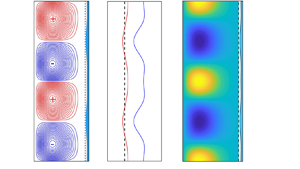
which fixes the amplitude of the perturbation. Computations indicate that the eigenfunction  $F_{11}$ is pure imaginary while $V_{11}$ is real. As an example, figure 5 shows the structure of the critical eigenfunctions obtained for a wide gap, $\eta = 0.4$. The main features are as follows. For small values of $0 \le B \le 0.88$, we have the case III basic solution: fully yielded fluid filling the annular gap. In this range of $B$, the maximum of $V_{11}$ and $F_{11}$ is shifted towards the inner wall, with a significant decrease of the maximum of $F_{11}$. As $B$ increases, the critical eigenfunctions are non-zero only in a progressively smaller yielded layer of width $(R_y - R_1)$.

Figure 5. Eigenfunctions (a)  ${\rm Im}(F_{11})$ and (b) $V_{11}$ associated with the critical mode at $\eta = 0.4$ for different values of $B$: 0, 0.2, 0.4, 0.6, 0.8, 1, 2, 3, 4, 5, 10.
As for the basic flow, it can be shown that every case II stability problem maps to a case II–III stability problem. This procedure is quite common in linear stability problems of viscoplastic fluid (Landry et al. Reference Landry, Frigaard and Martinez2006; Nouar et al. Reference Nouar, Kabouya, Dusek and Mamou2007). Indeed, if we rescale the radial distance as for the basic flow and use the definitions  $\tilde {k} = k (R_0 - R_1 )$, $\tilde {s} =s (R_0 - R_1)^2$, $\widetilde {Re}_1 = Re_1\,(R_0 - R_1)$ and $\widetilde {Re}_2 = Re_2\,R_0 (1 - \eta ) (R_0 - R_1 )$, then we recover an identical eigenvalue problem. The mapping was made possible because the boundary conditions are homogeneous (Landry et al. Reference Landry, Frigaard and Martinez2006).
In figure 6(a) we have represented the yield surface perturbations by the linear mode  $H_{11} E^1$, along the reduced axial position $z/\lambda _z$, where $\lambda _z = 2 {\rm \pi}/k_c$ is the axial wavelength. The case II of the base flow is considered with different values of the Bingham number. The minimum of ${\rm Re}(H_{11} E^1)$ corresponds to the jet impingement near the yield surface, and the maximum to the radial flow from the outer to the inner cylinder. It can also be noticed in figure 6(b) that $H_{11}$ decreases significantly with increasing Bingham number.

Figure 6. (a) Perturbation of the yield surface associated with the critical mode at  $\eta = 0.4$ for three different values of the Bingham number: (1) $B = 1$, (2) $B = 5$ and (3) $B = 10$. (b) Variation of $H_{11}$ as a function of $B$ for three different values of the radius ratio: (1) $\eta = 0.4$, (2) $\eta = 0.6$ and (3) $\eta = 0.8$. Vertical dashed lines indicate the value of $B$ from which a static layer appears on the outer cylinder.
4.2.2. Linear adjoint mode
The adjoint mode is required to obtain the Ginzburg–Landau equation. Its definition is given as
 \begin{equation} \left\langle\, \boldsymbol{f}_{ad}, \boldsymbol{L} \boldsymbol{f}_1\right\rangle = \left\langle \boldsymbol{L}_{ad}\kern1.5pt\boldsymbol{f}_{ad}, \boldsymbol{f}_1 \right\rangle , \end{equation}
where  $\boldsymbol {f}_{ad} = [F_{ad}, V_{ad} ]^{\rm T}$ is the adjoint eigenfunction, $\boldsymbol {L}$ is the linear stability operator, and $\boldsymbol {L}_{ad} = Re_1\, \boldsymbol {LI}_{ad} + \boldsymbol {LV}_{ad} + B \, \boldsymbol {LY}_{ad}$ is the corresponding adjoint operator. In this definition, the inner product is given as
 \begin{equation} \left\langle\, \boldsymbol{f}, \boldsymbol{g} \right\rangle = \int_{R_1}^{R_0} \boldsymbol{f}^* \boldsymbol{\cdot} \boldsymbol{g} \, r \,{\rm d} r , \end{equation}
where  $\boldsymbol {f}^*$ is the complex conjugate of $\boldsymbol {f}$. We find that $\boldsymbol {C}_{(\ell )}, \boldsymbol {LV}_{(\ell )}$ and $\boldsymbol {LY}_{(\ell )}$ ( $\ell = 0, 1, 2$) are real and self-adjoint, whereas $\boldsymbol {LI}_{(\ell )}$ is not self-adjoint. We have
 \begin{equation} \boldsymbol{LI}_{ad} = \begin{pmatrix} 0 & - {\rm i} k_c D_* V_b \\ 2 {\rm i} k_c V_b/r & 0\\ \end{pmatrix}. \end{equation}
The linear adjoint problem
 \begin{equation} \boldsymbol{L}_{ad}\left(\boldsymbol{f}_{ad} \right) = 0 \end{equation}
is subject to appropriate boundary conditions, matching those of the linear problem, i.e. (4.21), (4.22) and (4.23). As the adjoint is linear and can be scaled arbitrarily, we normalize the adjoint eigenfunctions so that the maximum of the adjoint azimuthal velocity is  $\max (V_{ad})=1$.
4.2.3. Solution at order $\delta ^2$: quadratic modes

At order  $\delta ^2$, the solution has two components. The first component, proportional to $|A|^2 E^0$, arises from the nonlinear interaction of the fundamental mode with its complex conjugate, and the second one, proportional to $A^2 E^2$, arises from the nonlinear interaction of the fundamental mode with itself.
First, consider mode  $0$, factor $|A|^2 E^0$.
This harmonic is a correction at the second order of the base flow. It is obtained by solving the system of equations
 \begin{equation} \boldsymbol{L}_{0}\,\boldsymbol{f}^{(0)}_2=-Re_{1c} \left[\boldsymbol{NI}\left(\boldsymbol{f}^{(1)}_1 |\,\boldsymbol{f}^{(-1)}_{1} \right) \right]_{|A|^2 E^0} - B \left[\boldsymbol{NY} \left(\boldsymbol{f}^{(1)}_1 |\,\boldsymbol{f}^{(-1)}_{1} \right)\right]_{|A|^2 E^0}, \end{equation}
where  $\boldsymbol {f}^{(-1)}_{1} = \boldsymbol {f}_1^{(1)*}$ is the complex conjugate of $\boldsymbol {f}^{(1)}_1$. As previously, the boundary conditions are of two types.
In case II of the base solutions, the no-slip condition at the walls gives
 \begin{equation} F_{02} = DF_{02} = V_{02} = 0 \quad \text{at} \ r = R_1, R_2 . \end{equation}
In case III of the base solutions, the boundary conditions and yield conditions at the yield surface lead to
 $$\begin{gather} F_{02} = DF_{02} = 0 \quad \text{at} \ {r = R_y} , \end{gather}$$
 $$\begin{gather} D^2 F_{02} =- \left[H_{11} D^3 F_{11}^* + H_{11}^* D^3 F_{11} \right] \quad \text{at} \ {r = R_y} , \end{gather}$$
 $$\begin{gather}V_{02} = H_{11} H_{11}^* D^2 V_b \quad \text{at} \ {r = R_y}. \end{gather}$$
As for the linear eigenfunction, the nonlinear corrections are computed numerically. The results show, as expected, that  $F_{02} = 0$, i.e. there is no radial or axial mean flow. The correction at the second order of the azimuthal velocity profile of the base state is illustrated by the profiles of $V_{02}$ represented in figure 7 for different values of $B$. Near the inner cylinder, $V_{02} < 0$, i.e. the azimuthal velocity is reduced, and near the outer cylinder or near the yield surface, $V_{02} > 0$, i.e. the azimuthal velocity is increased. Actually, the profiles of $V_{02}$ can be related to the outward and inward radial flows. The radial outward flow carries fluid particles with high azimuthal momentum from the inner cylinder, increasing the azimuthal velocity near the outer cylinder. The radial inward flow carries fluid particles with low azimuthal momentum from the outer cylinder, decreasing the azimuthal velocity near the inner cylinder. For a wide gap and in the case of a Newtonian fluid, the deficit of the azimuthal velocity is higher than the surplus. With increasing Bingham number, the opposite result is observed. Furthermore, the fluid is yielded in a smaller domain of width $(R_y - R_1)$. Cancelling artificially the nonlinear yield stress terms in (4.30) allows us to highlight the contribution of the nonlinear inertial terms (figure 8a) and vice versa, to highlight the contribution of the nonlinear yield stress terms (figure 8b) on the modification of the basic flow. The interaction of the fundamental mode with its complex conjugate through nonlinear yield stress terms accelerates the fluid in the whole yielded fluid domain. A positive correction of the basic azimuthal flow leads to a destabilizing effect and therefore may be considered as a precursor to the emergence of a subcritical bifurcation.

Figure 7. Wide gap geometry with  $\eta = 0.4$. Modification of the base flow at the second order in $\delta$ for $B = 0, 0.2, 0.4, 0.6, 0.8, 1, 2, 3, 4, 5, 10$.

Figure 8. Wide gap geometry with  $\eta = 0.4$. Modification of the base flow at the second order in $\delta$. (a) Contribution of the nonlinear inertia terms for $B = 0, 0.2, 0.4, 0.6, 0.8, 1, 2, 3, 4, 5, 10$. (b) Contribution of the nonlinear viscous terms for the same values of $B$.
$B$.
The perturbation of the yield surface by the mode  $\tilde {H}_{02} E^0$ is obtained from the yield condition and is given by
 \begin{equation} \tilde{H}_{02} D^2 V_b =- DV_{02} - \left[H_{11} D^2 V_{11}^* + H_{11}^* D^2 V_{11}\right] - H_{11} H_{11}^* D^3 V_b \quad \text{at} \ r = R_y , \end{equation}
with  $\bar {H}_{02} = H_{02} + \bar {H}_0$. The first term arises from the interaction of the fundamental mode with its complex conjugate, and the second term arises from the variation of the Bingham number as the Reynolds number is increased. The variation of $\tilde {H}_{02}$ with the Bingham number is shown in figure 9. Positive values of $\tilde {H}_{02}$ mean that the width of the plug zone is reduced. The reduction is weaker with increasing $B$. Nevertheless, one can highlight the high values of $\tilde {H}_{02}$ compared with $H_{11}$. This result shows that in the presence of a static layer, the nonlinear terms become significant quickly.

Figure 9. Modification at the second order in  $\delta$ of the width of the static layer as a function of the Bingham number: (1) $\eta = 0.4$, (2) $\eta = 0.6$ and (3) $\eta = 0.8$. Vertical dashed lines indicate the value of $B$ from which a static layer appears on the outer cylinder.
Now consider the mode 2 factor of  $A^2 E^2$.
The first harmonic mode is a solution of the system of equations
 \begin{equation} \boldsymbol{L}_{0}\,\boldsymbol{f}^{(2)}_2 =- Re_{1c} \left[\boldsymbol{NI} \left(\boldsymbol{f}_1^{(1)} |\,\boldsymbol{f}_1^{(1)} \right)\right]_{A^2 E^2} - B \left[\boldsymbol{NY} \left(\boldsymbol{f}_1^{(1)} |\,\boldsymbol{f}_1^{(1)} \right)\right]_{A^2 E^2} , \end{equation}
with the appropriate boundary conditions.
In case III of the base solutions, the no-slip condition at the walls gives
 \begin{equation} F_{22} = DF_{22} = V_{22} = 0 \quad \text{at} \ r = R_1, R_2 . \end{equation}
In case II of the base solutions, the boundary conditions and yield conditions at the yield surface lead to
 $$\begin{gather} F_{22} = DF_{22} = 0 \quad \text{at} \ r = R_y , \end{gather}$$
 $$\begin{gather}D^2F_{22} =- H_{11} D^3 F_{11}\quad \text{at} \ r = R_y , \end{gather}$$
 $$\begin{gather}V_{22} = \tfrac{1}{2}H_{11}^2 D^2 V_b \quad \text{at} \ r = R_y . \end{gather}$$
The influence of Bingham number  $B$ on the profiles ${\rm Im}(F_{22}(r))$ and $V_{22}(r)$ is shown in figure 10. The maximum of these profiles increases over a short range of $B$, where the fluid is fully yielded, and then decreases with increasing $B$, probably as a consequence of the reduction of energy exchange between the fundamental and its harmonic via the nonlinear yield stress terms.

Figure 10. Correction of the linear mode at the second order in  $\delta$ at critical conditions at $\eta = 0.4$ and for different values of $B$:
$B$:  $0, 0.2,0.6, 0.8, 1, 2, 3, 4, 5, 10$; (a) ${\rm Im}(F_{22}(r))$, and (b) $V_{22}(r)$.
The perturbation of the yield surface by the mode  $H_{22} A^2 E^2$ is obtained from yield conditions and is given by
 \begin{equation} H_{22} D^2 V_b =- DV_{22} - H_{11} D^2 V_{11} - \frac{H_{11}^2}{2}\,D^3 V_b \quad \text{at} \ r = R_y . \end{equation}
It is represented in figure 11 as a function of  $B$. One notices that: (i) $H_{22}$ decreases with increasing width of the static layer; and (ii) $H_{22}$ is one order of magnitude larger than $H_{11}$.
Remark As for the linear problem, there is a similarity mapping that maps  $V_{02}$, $F_{22}$ and $V_{22}$, obtained in the case where the fluid in the annular space is partially yielded, onto solutions $\tilde {V}_{02}$, $\tilde {F}_{22}=F_{22}/(R_0 - R_1)$ and $\tilde {V}_{22}$, obtained for an outer cylinder of radius equal to the yield surface radius.

Figure 11. (a) Yield surface perturbation of mode 2 for  $\eta = 0.4$ and three different values of $B$: (1) $B = 1$, (2) $B = 5$ and (3) $B = 10$. (b) Amplitude $H_{22}$ of the second harmonic of the yield surface perturbation as a function of the Bingham number: (1) $\eta = 0.4$, (2) $\eta = 0.6$ and (3) $\eta = 0.8$.
4.2.4. Solution at order $\delta ^3$: the Ginzburg–Landau equation

At order  $\delta ^3$, the solution has two components. The first, proportional to $|A|^2 A E^{1}$, represents the feedback at order $\delta ^3$ on the fundamental mode through the nonlinear interactions of the fundamental with the second harmonic, and with the modification of the basic state. The second component is the second harmonic.
The first component,  $\boldsymbol {f}^{(3)}_1 = [F_{13}, V_{13}]^{\rm T}$, satisfies the non-homogeneous equation
 \begin{align} |A|^2 A \boldsymbol{L}_{0}\,\boldsymbol{f}^{(1)}_3& = \boldsymbol{C}_{0}\,\frac{\partial A}{\partial T}\,\boldsymbol{f}^{(1)}_1 - Re^{(2)}\,A \left(\boldsymbol{LI}_{0} - \frac{B}{Re_c}\, \boldsymbol{LY}_{0} \right) \boldsymbol{f}^{(1)}_1 - A \, \boldsymbol{L}_{2}\, \boldsymbol{f}^{(1)}_1\nonumber\\ &\quad - Re_{1c}\,|A|^2 A \left[\boldsymbol{NI}\left(\boldsymbol{f}^{(1)}_1 |\,\boldsymbol{f}_2^{(0)} \right) + \boldsymbol{NI}\left(\boldsymbol{f}^{(-1)}_{1} |\,\boldsymbol{f}_2^{(2)} \right) \right] \nonumber\\ &\quad - B\, |A|^2 A \left[\boldsymbol{NY}\left(\boldsymbol{f}^{(1)}_1 |\,\boldsymbol{f}_2^{(0)} \right) + \boldsymbol{NY}\left(\boldsymbol{f}^{(-1)}_{1} |\,\boldsymbol{f}_2^{(2)} \right) \right] \nonumber\\ &\quad - B\,|A|^2 A\,\boldsymbol{NY} \left(\boldsymbol{f}_{1}^{(1)},\boldsymbol{f}_{1}^{(1)}|\,\boldsymbol{f}_{1}^{(-1)} \right) . \end{align}
Concerning the boundary conditions, for case III of the base solutions, we have
 $$\begin{gather} F_{13} = DF_{13} = 0 \quad \text{at} \ r = R_1, R_2 , \end{gather}$$
 $$\begin{gather}V_{13} =0\quad \text{at} \ r = R_1, R_2 . \end{gather}$$
For case II of the base solutions, the boundary conditions combined with the yield conditions at the yield surface are
 $$\begin{gather} F_{13} = 0 , \end{gather}$$
 $$\begin{gather}DF_{13} = H_{11} H_{11}^* D^3F_{11} + \frac{H_{11}^2}{2}\,D^3 F_{11}^* , \end{gather}$$
 $$\begin{gather}D^2F_{13} =- H_{11} H_{11}^* D^4 F_{11} - H_{11}^* D^3 F_{22} - \bar{H}_{02} D^3 F_{11} - H_{22} D^3 F_{11}^* \nonumber\\ {}\qquad \qquad - \frac{H_{11}^2}{2}\,D^4 F_{11}^* - \frac{H_{11}}{R_0} \left[H_{11}D^3 F_{11}^* + H_{11}^* D^3 F_{11} \right], \end{gather}$$
 $$\begin{gather}V_{13} = H_{11} H_{11}^* D^2 V_{11} + \frac{H_{11}^2}{2}\,D^2 V_{11}^* + H_{11}^2 H_{11}^* D^3 V_b \nonumber\\ {}+ \left(H_{11}^* H_{22} + H_{11} \bar{H}_{02} \right) D^2 V_b . \end{gather}$$
The condition on  $DV_{13}$ defines $H_{13}$, but is lengthy and omitted for brevity.
The amplitude equation is found in the usual way, as a solvability condition on the third-order problem. In the case where the annular space is fully yielded, the boundary conditions for  $\boldsymbol {f}_1^{(3)}$ are homogeneous. The solvability condition leads to
 \begin{align} 0&= \left\langle\, \boldsymbol{f}_{ad}, \boldsymbol{C}_{0}\,\boldsymbol{f}^{(1)}_1 \right\rangle \frac{\partial A}{\partial T}\nonumber\\ &\quad - Re^{(2)} \left\langle\, \boldsymbol{f}_{ad}, \left(\boldsymbol{LI}_{0} - \frac{B}{Re_{1c}}\, \boldsymbol{LY}_{0} \right) \boldsymbol{f}^{(1)}_1 \right\rangle A - \left\langle\, \boldsymbol{f}_{ad}, \boldsymbol{L}_{2}\, \boldsymbol{f}^{(1)}_1 \right\rangle A \nonumber\\ &\quad - Re_{1c} \left\langle\, \boldsymbol{f}_{ad}, \boldsymbol{NI} \left(\boldsymbol{f}^{(0)}_2|\,\boldsymbol{f}^{(1)}_1\right)\right\rangle |A|^2 A - Re_{1c} \left\langle\, \boldsymbol{f}_{ad}, \boldsymbol{NI} \left(\boldsymbol{f}^{(2)}_2|\,\boldsymbol{f}^{(-1)}_{1}\right)\right\rangle |A|^2 A \nonumber\\ &\quad - B \left\langle\, \boldsymbol{f}_{ad}, \boldsymbol{NY} \left(\boldsymbol{f}^{(0)}_2|\,\boldsymbol{f}^{(1)}_1\right)\right\rangle |A|^2 A - B \left\langle\, \boldsymbol{f}_{ad}, \boldsymbol{NY} \left(\boldsymbol{f}^{(2)}_2|\,\boldsymbol{f}^{(-1)}_{1}\right)\right\rangle |A|^2 A \nonumber\\ &\quad - B \left\langle\, \boldsymbol{f}_{ad}, \boldsymbol{NY} \left((\boldsymbol{f}^{(1)}_1,\boldsymbol{f}^{(1)}_1) |\,\boldsymbol{f}^{(-1)}_{1}\right)\right\rangle |A|^2 A . \end{align}
Using the departure from the linear threshold
 \begin{equation} \epsilon = \frac{Re_1 - Re_{1c}}{Re_{1c}} = \delta^2\,\frac{Re^{(2)}}{Re_{1c}}, \end{equation}
and after returning to the fast variables
 \begin{equation} \delta A(Z,T) = A'(z,t),\quad \frac{\partial}{\partial Z} = \frac{1}{\delta}\,\frac{\partial}{\partial z}\quad \text{and}\quad \frac{\partial}{\partial T} = \frac{1}{\delta^2}\,\frac{\partial}{\partial t}, \end{equation}
the following Ginzburg–Landau equation is derived:
 \begin{equation} \frac{\partial A}{\partial T} = \frac{\epsilon}{\tau_0}\,A + \frac{\xi_0^2}{\tau_0}\,\frac{\partial^2 A}{\partial z^2} + g_1\,|A|^2 A. \end{equation}
In (4.52), we have dropped the prime in  $A'$ and we expect no confusion to the reader. In this equation, $\tau _0$ is the characteristic time for the instability to grow,
 \begin{equation} \displaystyle \tau_0^{-1} = Re_{1c}\,\frac{\left\langle\, \boldsymbol{f}_{ad}, \left(\boldsymbol{LI}_0 - \displaystyle \dfrac{B}{Re_{1c}}\,\boldsymbol{LY}_0 \right) \boldsymbol{f}_1^{(1)}\right\rangle}{\left\langle\, \boldsymbol{f}_{ad}, \boldsymbol{C}_0\, \boldsymbol{f}_1^{(1)} \right\rangle}, \end{equation} $\xi _0$ is the coherence length,
 \begin{equation} \xi_0^2 = \frac{1}{Re_{1c}}\,\displaystyle \frac{\left\langle\, \boldsymbol{f}_{ad}, \boldsymbol{L}_2 \boldsymbol{f}_1^{(1)}\right\rangle}{\left\langle\, \boldsymbol{f}_{ad}, \left(\boldsymbol{LI}_0 - \displaystyle \dfrac{B}{Re_{1c}}\,\boldsymbol{LY}_0 \right) \boldsymbol{f}_1^{(1)} \right\rangle}, \end{equation}
and  $g_1$ is the first Landau coefficient,
 \begin{align} g_1 &= Re_{1c}\,\frac{\left\langle\, \boldsymbol{f}_{ad}, \boldsymbol{NI} \left(\boldsymbol{f}^{(0)}_2|\,\boldsymbol{f}^{(1)}_1\right)\right\rangle}{\left\langle\, \boldsymbol{f}_{ad}, \boldsymbol{C}_{0}\,\boldsymbol{f}^{(1)}_1 \right\rangle} + Re_{1c}\, \frac{\left\langle\, \boldsymbol{f}_{ad}, \boldsymbol{NI} \left(\boldsymbol{f}^{(2)}_2|\,\boldsymbol{f}^{(-1)}_{1}\right)\right\rangle}{\left\langle\, \boldsymbol{f}_{ad}, \boldsymbol{C}_{0}\,\boldsymbol{f}^{(1)}_1 \right\rangle}\nonumber\\ &\quad+ B\,\frac{\left\langle\, \boldsymbol{f}_{ad},\boldsymbol{NY} \left(\boldsymbol{f}^{(0)}_2|\,\boldsymbol{f}^{(1)}_1\right)\right\rangle}{\left\langle\, \boldsymbol{f}_{ad}, \boldsymbol{C}_{0}\,\boldsymbol{f}^{(1)}_1 \right\rangle} + B\, \frac{\left\langle\, \boldsymbol{f}_{ad}, \boldsymbol{NY} \left(\boldsymbol{f}^{(2)}_2|\,\boldsymbol{f}^{(-1)}_{1}\right)\right\rangle}{\left\langle\, \boldsymbol{f}_{ad}, \boldsymbol{C}_{0}\,\boldsymbol{f}^{(1)}_1 \right\rangle} \nonumber\\ &\quad + B\,\frac{\left\langle\, \boldsymbol{f}_{ad}, \boldsymbol{NY} \left((\boldsymbol{f}^{(1)}_1,\boldsymbol{f}^{(1)}_1) |\,\boldsymbol{f}^{(-1)}_{1}\right)\right\rangle}{\left\langle\, \boldsymbol{f}_{ad}, \boldsymbol{C}_{0}\,\boldsymbol{f}^{(1)}_1 \right\rangle}. \end{align}
 The integrals are evaluated numerically by means of the Clenshaw and Curtis method (Trefethen Reference Trefethen2000). At critical conditions, and assuming that the amplitude does not vary with the axial position,  $\boldsymbol {f}_1^{(3)} = \boldsymbol {f}_{1H}^{(3)}$ satisfies an equation of the form
 \begin{equation} \boldsymbol{L}_0\, \boldsymbol{f}_{1H}^{(3)} = g_{1H} \boldsymbol{C}_0\, \boldsymbol{f}_1^{(1)} - Re_{1C}\,\boldsymbol{NI} - B\,\boldsymbol{NY}. \end{equation}
In the case where there is a static layer on the outer wall, the boundary conditions at the yield surface (defined in (4.46)–(4.48)) are inhomogeneous. In order to derive the solvability condition, we decompose, as in Sen & Venkateswarlu (Reference Sen and Venkateswarlu1983) and Bouteraa et al. (Reference Bouteraa, Nouar, Plaut, Métivier and Kalck2015),  $\boldsymbol {f}_1^{(3)}$ into homogeneous ( $\boldsymbol {f}^{(3)}_{1H}$) and inhomogeneous ( $\boldsymbol {f}^{(3)}_{1NH}$) parts:
 \begin{equation} \boldsymbol{f}_1^{(3)} = \boldsymbol{f}^{(3)}_{1H} + \boldsymbol{f}^{(3)}_{1NH}, \end{equation}
where  $\boldsymbol {f}^{(3)}_{1NH}$ is a correction term that accounts for the non-homogeneity of the boundary conditions. Furthermore, at critical conditions, $\boldsymbol {f}_1^{(3)}$ satisfies an equation that can be written as
 \begin{equation} \boldsymbol{L}_0\, \boldsymbol{f}_{1}^{(3)} = g_{1} \boldsymbol{C}_0\, \boldsymbol{f}_1^{(1)} - Re_{1C}\,\boldsymbol{NI} - B\,\boldsymbol{NY}. \end{equation}
Substituting (4.57) into (4.58), we obtain
 \begin{equation} \boldsymbol{L}_0\, \boldsymbol{f}_{1H}^{(3)} = g_{1} \boldsymbol{C}_0\, \boldsymbol{f}_1^{(1)} - Re_{1C}\,\boldsymbol{NI} - B\,\boldsymbol{NY} - \boldsymbol{L}_0\, \boldsymbol{f}_{1H}^{(3)}. \end{equation}
By applying the solvability condition to (4.59), we get
 \begin{equation} g_1 = g_{1H} + \frac{\left\langle\, \boldsymbol{f}_{ad}, \boldsymbol{L}_0\, \boldsymbol{f}_{1NH}^{(3)} \right\rangle}{\left\langle\, \boldsymbol{f}_{ad}, \boldsymbol{C}_{0}\,\boldsymbol{f}^{(1)}_1 \right\rangle} . \end{equation}
The technique of solution adopted is to iterate a few times between (4.57) and (4.60). At the start,  $\boldsymbol {f}_{1NH}^{(3)}$ is assumed to be identically zero in (4.60). A first approximation of $g_1$ is then obtained: $g_1^{(1)} = g_{1H}$. This is put into (4.58), which is solved at the critical conditions, with non-homogeneous boundary conditions, to obtain a first approximation of $\boldsymbol {f}_1^{(3)}$. Using (4.57), a first approximation of $\boldsymbol {f}_{1NH}^{(3)}$ is deduced. Then $\boldsymbol {f}_{1NH}^{(3)}$ is put into (4.60). This process is repeated until it converges to a desired level of accuracy. Note that (4.58) is solved with an additional condition
 \begin{equation} \boldsymbol{f}_{1}^{(3)} = 0 \quad \text{at} \ r = r_{max}, \end{equation}
where  $r_{max}$ is the radial position at which $V_{11}(r_{max})=1$. This normalization was suggested by Herbert (Reference Herbert1980, Reference Herbert1983), Sen & Venkateswarlu (Reference Sen and Venkateswarlu1983) and Generalis & Fujimura (Reference Generalis and Fujimura2009). Without this normalization, $\boldsymbol {f}_{1}^{(3)}$ is defined up to an arbitrary multiple of the solution $\boldsymbol {f}_{1}^{(1)}$. A validation of the procedure used is provided in § 5 of the supplementary material.
5. Results and discussion
5.1. Characteristic time of instability growth and coherence length
The variation of the characteristic time  $\tau _0$, for the instability to grow, as a function of the Bingham number is shown in figure 12(a). As can be observed, $\tau _0$ decreases with increasing $B$ in particular when there is a static layer attached to the outer cylinder, i.e. for $B>0.88$ at $\eta =0.4$, and for $B > 8.5$ at $\eta = 0.883$. This result shows that the onset of Taylor vortex flow is faster with increasing $B$, and even more in the presence of a plug zone on the outer cylinder. To account for the reduction of the annular space in the presence of a static layer on the outer cylinder, $\tau _0$ and $B$ can be rescaled as $\tilde {B}= B (R_y - R_1)$ and $\tilde {\tau }_0 = \tau _0 / (R_y - R_1) ^2$. In the representation of $\tilde {\tau }_0$ as a function of $\tilde {B}$, the slope of the curve is reduced substantially.

Figure 12. Variations of (a) the characteristic time of instability and (b) the coherence length as functions of the Bingham number for narrow and wide gaps: (1)  $\eta = 0.883$, (2) $\eta = 0.4$.
Similarly, the coherence length, which can be related to the curvature of the marginal stability curve, decreases with increasing  $B$ as shown in figure 12(b). This means that the marginal stability curve flattens with increasing $B$. The strong decrease of $\xi _0$ with increasing $B$, for $B > 0.88$ at $\eta = 0.4$, accounts for the reduction of the width of the annular space where the fluid is yielded. This can be taken into account by using the rescaled parameter $\tilde {B}$ and $\tilde {\xi }_0 = \xi _0/(R_y - R_1)^2$.
5.2. Transition from supercritical to subcritical bifurcation
In figures 13(a,b), we have represented the variation of the first Landau constant  $g_1$ as a function of the Bingham number for different values of the radius ratio $\eta$, with $Re_2 = 0$. The sign of $g_1$ determines whether we are dealing with a supercritical or a subcritical bifurcation. The following characteristics are noticed.
(i) For a given radius ratio and at
$B=0$ (Newtonian fluid), $g_1$ is negative and the bifurcation is supercritical. With increasing $B$, $g_1$ decreases, reaches a minimum, then increases rapidly until a particular value of $B$ where the convexity of $g_1(B)$ changes abruptly. Actually, at this particular value of $B$, a static layer appears on the outer wall.(ii) From
$\eta \ge \eta _{\ell }$, with $\eta _{\ell } = 0.89$ in the present case (thick curve in figure 13a), $g_1$ is negative and the bifurcation is supercritical for the whole range of values of $B$ considered.(iii) For
$\eta < \eta _{\ell }$, $g_1$ is positive and the bifurcation is subcritical for a range of Bingham numbers whose extent is all the larger as the annular gap is wide. This is illustrated by figure 13(c) where we have represented in the plane $(\eta, B)$ the boundaries of the subcritical bifurcation domain. Outside this domain, the bifurcation is supercritical.(iv) The numerical results show that at the upper boundary of the subcritical bifurcation domain (numbered (3) in figure 13c), the inner to the yield surface radius ratio is
$R_1/R_y \approx \eta _{\ell }$. In other words, when $R_1/R_y > \eta _{\ell }$, the bifurcation is supercritical.(v) At the lower boundary of the subcritical bifurcation domain (numbered (1) in figure 13c),
$R_1/R_y = 0.6$. Hence for $\eta < 0.6$, subcritical bifurcation occurs only in presence of a static layer on the outer wall.(vi) The minimum value of
$B$ at which the primary bifurcation is subcritical is $B=1.8$, obtained for $\eta = 0.6$.


Figure 13. Variation of the first Landau constant as a function of the Bingham number for different values of the radius ratios: (a) from  $\eta = 0.92$ until $\eta = 0.81$ by step $0.01$, and then $\eta = 0.79, 0.77, 0.75, 0.73, 0.7, 0.66, 0.6$; (b) $\eta = 0.6, 0.5, 0.4$. (c) Boundaries of the subcritical domain in the plane ( $\eta, B$): (1) and (2) are the lower boundaries, and (3) is the upper boundary.
To shed more light on the mechanism of supercritical/subcritical instability, the first Landau constant is decomposed as
 \begin{equation} \displaystyle g_1 = g_{1I} + g_{1Y} + g_{1 NH}, \end{equation}
where  $g_{1I}$ is the contribution of nonlinear inertial terms (terms where $Re_{1c}$ is a factor in (4.55)), $g_{1Y}$ is the contribution of nonlinear yield stress terms (terms where $B$ is a factor in (4.55)), and $g_{1NH}$ is the contribution of non-homogeneous boundary conditions. In figure 14, we have represented the contribution of nonlinear inertial terms and nonlinear yield stress terms to the first Landau constant for different values of $\eta$. One can notice the following.
(i) The value of
$g_{1I}$ is negative, and $g_{1Y}$ is positive, i.e. the nonlinear inertial terms promote a supercritical bifurcation leading to saturation of the stationary instability at finite amplitude, whereas the nonlinear yield stress terms promote a subcritical bifurcation. The position of the curve $-g_{1I}$ relative to $g_{1Y}$ accounts for the nature of the primary bifurcation described in figure 13(a). For $\eta \ge \eta _{\ell } = 0.89$ (figures 14a,b), $(-g_{1I}) > g_{1Y}$ and the bifurcation is supercritical. For $\eta < \eta _{\ell }$ (figures 14c,d), $(-g_{1I}) > g_{1Y}$ for a range of $B$ close to zero and for large values of $B$. For intermediate values of $B$, i.e. between the two crossings of the curves $-g_{1I}(B)$ and $g_{1Y}(B)$ (figure 14c), the bifurcation is subcritical.(ii) The values of
$(-g_{1I})$ and $g_{1Y}$ increase with $B$ but differently depending on whether the annular space is fully or partially yielded.(iii) The abrupt change in the convexity of
$g_1(B)$ observed in figures 13(a,b) arises from the change in the curvature of $g_{1Y}(B)$ when a static layer appears on the outer cylinder.(iv) As for the non-homogeneous boundary conditions, the obtained values of
$g_{1NH}$ show that they promote a subcritical bifurcation. However, their contribution remains very weak, almost $10^{-3}$ smaller than ($-g_{1I}$), as is shown in figure 7 of the supplementary material. Therefore, $g_{1NH}$ does not play a significant role in the transition from supercritical to subcritical bifurcation.


Figure 14. Contributions of nonlinear inertial terms  $g_{1I}$ and nonlinear yield stress terms $g_{1Y}$ on the first Landau constant as a function of $B$ for (a) $\eta = 0.92$, (b) $\eta = 0.89$, (c) $\eta = 0.88$, and (d) $\eta = 0.6$.
Obviously, the increase of  $-g_{1I}$ with increasing $B$ has to be due to changes with $B$, in either $Re_{1c}$ or in the factor term of $Re_{1c}$ in (4.55). This last term contains quadratic products of the eigenfunctions and their derivatives that are non-zero in a progressively smaller yielded fluid domain. The numerical results show that more than $99\,\%$ of the variation of $g_{1I}$ arises from the variation of $Re_{1c}$ as $B$ increases. Furthermore, it is observed that $-g_{1I}$ can be fitted by an affine function of $Re_{1c}$, with different coefficients, in partially and fully yielded domains. The factor term of $Re_{1c}$ in (4.55) varies mainly with $\eta$.
Regarding the variation of  $g_{1Y}$ with $B$, where $g_{1Y}$ can be written formally as $g_{1Y}=B \langle \boldsymbol {f}_{ad}, \boldsymbol {NY}\rangle / \langle \boldsymbol {f}_{ad}, \mathcal {C}_0 \boldsymbol {f}^{(1)} \rangle$, two situations must be distinguished, depending on whether the annular space is fully or partially yielded.
The first situation, where the annular space is fully yielded, is as we have a purely viscous shear-thinning fluid. The numerical results show that the increase of  $g_{1Y}$ with increasing $B$ can be fitted by a cubic polynomial. The nonlinear yield stress term $\boldsymbol {NY}$ derived from $mk_{ij}$ expressions (2.31)–(2.36) contains products of eigenfunctions and their derivatives divided by $\dot {\gamma }^{k}(\boldsymbol {U}_b)$ ( $k=1,2,3$). It is precisely these terms, i.e. $1/\dot {\gamma }^{k}(\boldsymbol {U}_b)$, that are responsible for the strong increase in $g_{1Y}$ with increasing $B$. Indeed, at the outer wall and at critical conditions, $\dot {\gamma }(\boldsymbol {U}_b)|_{R_2}$ decreases linearly with increasing $B$, and tends to zero as $B$ approaches $B_{s\ell }$, the value of $B$ at which a static layer appears at the outer wall, i.e. $\dot {\gamma }(\boldsymbol {U}_b)|_{R_2} \propto (B_{s \ell } - B)$. Therefore, $1/\dot {\gamma }(\boldsymbol {U}_b)|_{R_2}$ increases sharply, allowing the nonlinear yield stress term to become dominant as $B \to B_{s\ell }$.
In the second situation, where the annular space is partially yielded,  $g_{1Y}$ increases linearly with $B$. The quantity $\langle \boldsymbol {f}_{ad}, \boldsymbol {NY}\rangle / \langle \boldsymbol {f}_{ad}, \mathcal {C}_0 \boldsymbol {f}^{(1)} \rangle$ remains almost constant as $B$ increases. Here, the characteristics of the flow just after yielding, where $\dot {\gamma }(\boldsymbol {U}_b) \to 0$, play the dominant role. Recall that the compatibility conditions (equations (4.8)–(4.13) of the supplementary material) ensure that the limit of $\boldsymbol {NY}$ is finite when $\dot {\gamma }(\boldsymbol {U}_b)$ tends to zero.
Remarks
(i) A detailed study of the contribution of the different terms that intervene in the
$g_{1I}$ and $g_{1Y}$ expressions (4.55) is provided in § 5 of the supplementary material. The data show that the feedback of the mean flow correction plays an important role.(ii) For counter-rotating and co-rotating cylinders, variations of the first Landau constant
$g_1$, the contribution of nonlinear inertial terms $g_{1I}$ and that of nonlinear yield stress terms $g_{1Y}$ as a function of the Bingham number, are qualitatively similar to those obtained for a fixed outer cylinder. They are described in §§ A.1 and A.2.


5.3. Stationary amplitudes
A steady solution of (4.52) is
 \begin{equation} A = A_0 {\rm e}^{{\rm i} q z}, \quad \text{with} \ A_0 = \left|{\frac{\epsilon - \xi_0^2 q^2}{\tau_0 (-g_1)}}\right|^{1/2} \ \text{and} \ q = k-k_c . \end{equation}
 Figure 15 shows the bifurcation diagram obtained in the case where  $k = k_c$, i.e. $q=0$, at different Bingham numbers. For a wide gap, $\eta = 0.4$, near the critical conditions, the stable stationary equilibrium amplitude in the supercritical regime is shown in continuous line. At low values of $B$ (
$B$ ( $B\leq 0.5$), the nonlinearities dominated by the nonlinear inertial terms are stabilizing. The nonlinear effects associated with the viscosity perturbation, i.e. $NY$ terms, start to become significant from $B = 0.5$ (minimum of $g1(B)$), leading to a strong increase of the amplitude as $B$ increases. This effect becomes more pronounced from a Bingham number $B = 0.88$ at which a static layer appears on the outer cylinder, with a strong decrease of $\tau _0$ with increasing $B$. When the bifurcation is subcritical, the threshold amplitude, which limits the basin of attraction of the circular Couette flow, shown in dashed line, decreases with increasing $B$, i.e. the basic flow becomes more sensitive to finite-amplitude perturbations. However, this variation cannot continue. Indeed, when the width of the yielded zone is sufficiently narrow, $R_1/R_y \ge \eta _{\ell }$ ( $\eta _{\ell } = 0.89$ when the outer cylinder is fixed), the bifurcation again becomes supercritical. For a narrow gap, here $\eta = 0.883$, similar effects are observed in overall (see figure 15b), except that the nonlinear terms $NY$ start to become significant from $B = 4$, with a significant increase in amplitude as $B$ increases. The appearance of a static layer at the outer cylinder occurs in the subcritical domain, and the return to a supercritical bifurcation takes place at $B = 9$.

Figure 15. Stationary amplitude as a function of the distance  $\epsilon$ to criticality. (a) Wide gap, $\eta = 0.4$: (1) $B = 0$, (2) $B = 0.5$, (3) $B = 0.8$, (4) $B = 1$, (5) $B = 2$, (6) $B = 3$, (7) $B = 6$, (8) $B = 8$, (9) $B = 10$. (b) Narrow gap, $\eta = 0.883$: (1) $B = 0$, (2) $B = 1$, (3) $B = 5$, (4) $B = 7$, (5) $B = 8$, (6) $B = 12$.
5.4. Flow structure
One has to note that the numerical values of the Landau constant, and hence the values of the amplitude, depend on the normalization condition used for the eigenfunctions in the linear theory. However, physical quantities such as velocity components, kinetic energy or torque are independent of the normalization. In figure 16, we have represented the profiles of the radial velocity component
 \begin{equation} u=- \left({\rm i} k_c A F_{11} E^1 + 2 {\rm i} k_c A^2 F_{22}^* E^2 + {\rm c.c.}\right) + O(A^3) \end{equation}
at  $z=0$, $\epsilon = 0.01$, in a wide gap and a narrow gap, and for different Bingham numbers. These profiles represent the outward radial flow between the inner and outer cylinders, near the onset of the Taylor vortex flow regime. For values of $B$ small enough comparatively to that for which a plug zone appears on the outer cylinder, the increase of $|g_{1I}|$ with $B$ is much more significant than that of $g_{1Y}$ with $B$ (figure 14), and overall, $|g_{1}|$ increases (figure 13), leading to a decrease in the perturbation amplitude (5.2) and therefore to that of the radial velocity as $B$ increases; see curves (1) and (2) in figure 16(a), and curves (1), (2) and (3) in figure 16(b). However, as $B$ approaches the value associated with the appearance of the plug zone, the increase in $g_{1Y}$ with $B$ (parabolic) becomes significant, and overall, the value of $|g_1|$ begins to decrease, resulting in an increase in amplitude, and thus an increase in the radial velocity; see curves (3) and (4) in figure 16(a), and curves (4) and (5) in figure 16(b).

Figure 16. Radial velocity component  $u$ across the gap at $z = 0$, $\epsilon = 0.01$, $Re_2 = 0$ and for different Bingham numbers. (a) Wide gap, $\eta = 0.4$: (1) $B = 0$, (2) $B = 0.5$, (3) $B = 0.8$, (4) $B = 1$. (b) Narrow gap, $\eta = 0.883$: (1) $B = 0$, (2) $B = 1$, (3) $B = 5$, (4) $B = 7$, (5) $B = 7.2$.
The evolutions of the axial velocity profiles as functions of  $B$ follow the same trends as those described for $u$. They are therefore not shown.
Outward and inward radial flows carry high azimuthal momentum fluxes from near the inner to the outer cylinder, and low momentum fluxes from near the outer to the inner cylinder, respectively. These result in the formation of positive and negative azimuthal streaks. They are determined by the azimuthal velocity expression
 \begin{equation} v = A V_{11} + A^2 V_{22} + |A|^2 V_{02} + {\rm c.c.} + O(A^3). \end{equation}
Again, at low values of  $B$, the nonlinear inertial terms are dominant and have a stabilizing effect. Once, the nonlinear yield stress terms become significant, the intensity of the azimuthal streaks increases strongly with $B$, and even more in the presence of a static layer, as shown in figure 17.

Figure 17. Azimuthal velocity component  $v$ across the gap at $z=0$, $\epsilon = 0.01$, $Re_2 = 0$ and for different Bingham numbers. (a) Wide gap, $\eta = 0.4$: (1) $B = 0$, (2) $B = 0.5$, (3) $B = 1$, (4) $B = 1.4$. (b) Narrow gap, $\eta = 0.883$: (1) $B = 0$, (2) $B = 1$, (3) $B = 5$, (4) $B = 7$, (5) $B = 7.2$.
The change in the flow structure when departing from the critical conditions modifies the second invariant  $\dot {\gamma }$ of the strain rate tensor $\dot {\boldsymbol {\gamma }}$ and thus the effective viscosity.
In figure 18, we show the contours of the stream function  $\psi = r \phi$ at $\epsilon = 0.5 \times 10^{-2}$ (figure 18a), which will serve as a guide for the description of the results, and the contours of $\dot {\gamma }$ at $\epsilon = 0$ (figure 18b) and at $\epsilon = 0.5 \times 10^{-2}$ (figure 18c). The case of a wide gap, $\eta = 0.5$, is considered with stationary outer cylinder and $B = 1$ (fluid partially yielded). At the onset of Taylor vortices ( $\epsilon = 0$), $\dot {\gamma } = \dot {\gamma }_b(r)$ decreases monotonically from the inner wall to the yield surface represented by a dashed line. At $\epsilon = 0.5 \times 10^{-2}$, in the outward radial flow region, i.e. at approximately $z / \lambda _z =1$, we have $\dot {\gamma } < \dot {\gamma }_b$ near the inner wall, $\dot {\gamma } = \dot {\gamma }_b$ around the centre of the vortices, and $\dot {\gamma } > \dot {\gamma }_b$ at further radial positions. Opposite behaviours are observed in the inward radial flow region, i.e. at approximately $z/ \lambda _z =0.5$ and $1.5$.

Figure 18. Wide gap,  $\eta = 0.4$, with $B=1$ and stationary outer cylinder. (a) Contours of the stream function $\psi = r \phi$ at $\epsilon = 0.5\times 10^{-2}$: $+$ indicates clockwise rotation, $-$ indicates anticlockwise rotation. The dashed line indicates the position of the yield surface at critical conditions. (b) Contours of the second invariant $\dot {\gamma }$ of the strain rate tensor $\dot {\boldsymbol {\gamma }}$ at the onset of Taylor vortices, $\epsilon = 0$. (c) Contours of $\dot {\gamma }$ at $\epsilon = 0.5 \times 10^{-2}$.
Actually, an analysis of the different  $\dot {\gamma }_{ij}(\boldsymbol {U}_b + \boldsymbol {u})$ shows that $\dot {\gamma }$ is dominated by $|\dot {\gamma }_{r \theta } (\boldsymbol {U}_b + \boldsymbol {u})|$. In the outward radial flow region, $\dot {\gamma }_{r \theta } (\boldsymbol {u})$ is positive and maximum at the inner wall ( $\dot {\gamma } < \dot {\gamma }_b$); it decreases and vanishes around the centre of the Taylor vortices ( $\dot {\gamma } = \dot {\gamma }_b$), and then becomes negative ( $\dot {\gamma } > \dot {\gamma }_b$). Of course, in the regions where $\dot {\gamma } > \dot {\gamma }_b$, we have $\mu < \mu _b$ and vice versa.
5.5. Perturbation of the yield surface
For a sufficiently large Bingham number, a static layer forms and adheres to the outer cylinder. Near the onset of the Taylor vortex flow regime, the disturbed yield surface is given by
 \begin{equation} r = R_y + A H_{11} E^1 + {\rm c.c.} + \left|A\right|^2 \tilde{H}_{02} + A^2 H_{22} E^2 + {\rm c.c.} + O(A^3) . \end{equation}
In figure 19, we have represented contours of the stream function (figure 19a), the deformation of the yield surface (figure 19b), and contours of the azimuthal component of the velocity disturbance (figure 19c). The radius ratio is  $\eta = 0.4$, the Bingham number is $B = 1$, and the outer cylinder is stationary. In figure 19(b) a zoom is made on the modification of the yield surface. At critical conditions, the yield surface is represented in a dashed line, and its modification near the onset of vortices in continuous lines. On average, over one wavelength and at second order in amplitude, the thickness of the static layer is reduced by $|A|^2 \tilde {H}_{02}$. This reduction is due on the one hand to the increase in $Re_1$, i.e. an increase of the speed of the inner cylinder, and on the other hand to the interaction of the fundamental mode with its complex conjugate. The numerical results show that less than $7\,\%$ of the reduction in the static layer thickness is due to the increase in $Re_1$, and the remainder is due to the interaction of the fundamental mode with its complex conjugate. More precisely, it is observed that the erosion of the static layer arises mainly from the nonlinear yield stress terms. Indeed, if these nonlinear terms are cancelled artificially, then the erosion will be reduced substantially, as illustrated by curves (1) and (2) in figure 19(b).

Figure 19. Wide gap,  $\eta = 0.4$, with stationary outer cylinder, $B = 1$ and $\epsilon = 0.5\times 10^{-2}$. (a) Contours of the stream function. The dashed line indicates the position of the yield surface at critical conditions. (b) Zoom on the modification of the yield surface: (1) nonlinear yield stress terms are cancelled artificially; (2) nonlinear yield stress terms are taken into account. (c) Contours of azimuthal velocity perturbations: blue indicates negative azimuthal streaks; yellow indicates positive azimuthal streaks.
Around the average radius of the yield surface  $R_y +|A|^2 \tilde {H}_{02}$, a disturbance of small amplitude occurs due to the fundamental mode $A H_{11} E^1 + {\rm c.c.}$ and to the second harmonic (interaction of the fundamental with itself) $A^2 H_{22} E^2 + {\rm c.c.}$. This disturbance of the yield surface shows a ‘hump’ in the region where there is an inward radial flow with a negative azimuthal streak (blue contours in figure 19c) and a ‘trough’ in the region where there is an outward radial flow with a positive azimuthal streak (yellow contours). However, this disturbance around the average radius is quite weak comparatively to the reduction of the width of the plug layer.
Qualitatively similar results are obtained for a higher Bingham number, as shown in figure 20 for  $B = 1.4$. However, for the same relative distance to the onset of Taylor vortices, the erosion of the static layer is less pronounced for a larger static layer width.

Figure 20. Wide gap,  $\eta = 0.4$, with stationary outer cylinder, $B=1.4$ and $\epsilon = 0.5\times 10^{-2}$. (a) Contours of the stream function. (b) Zoom on the modification of the yield surface: (1) nonlinear yield stress terms are cancelled artificially; (2) nonlinear yield stress terms are taken into account. (c) Contours of azimuthal velocity perturbations: blue indicates negative azimuthal streaks; yellow indicates positive azimuthal streaks.
6. Conclusion
The present work focuses on the first principles in understanding the influence of the yield stress on the stability of a circular Couette flow with respect to a finite-amplitude perturbation. A weakly nonlinear analysis based on the multiple scales method is used as a first approach to take into account nonlinear effects. A Bingham model is used as a typical model of yield stress fluids. A detailed mathematical analysis is provided in the case where the base flow has a plug zone attached to the outer cylinder. The Ginzburg–Landau equation is derived, and the cubic Landau coefficient is determined for a wide range of Bingham numbers and different radius ratios. The character of the primary bifurcation results from the competition between nonlinear inertia terms that favour a supercritical bifurcation, and nonlinear yield stress terms that favour a subcritical bifurcation. The nonlinear inertia terms are dominant either in the case where the Bingham number is close to zero or in the case where the annular space is sufficiently narrow, i.e. the radius ratio is greater than a limit value  $\eta _{\ell }$, or equivalently, when the yielded fluid domain is sufficiently narrow, $R_1/R_y > \eta _{\ell }$. However, when $\eta < \eta _{\ell }$, the nonlinear yield stress terms become dominant and the bifurcation becomes subcritical for a range of $B$, the extent of which depends on $Re_2$ and $\eta$. To our knowledge, such variations in the nature of the primary bifurcation with $B$ and $\eta$ were not observed previously in the literature. Concerning the flow structure in the supercritical regime, it is shown that at low values of $B$, i.e. when the nonlinear inertial terms are dominant, the strength of the vortices decreases slightly with increasing $B$. However, once the nonlinear yield stress terms that account for the viscosity perturbation start to become significant, the strength of the vortices increases strongly with increasing $B$. This effect is more pronounced in the presence of a static layer.
Our analysis provides information about the first stages in the evolution of the yield surface when departing from the critical conditions. It is shown that the static layer is reduced due to the increase in the velocity of the inner cylinder and the interaction of the fundamental mode with its complex conjugate involving nonlinear yield stress terms. The contribution of the second effect is much greater than that of the first one. Furthermore, the yield surface is sinusoidally disturbed by the fundamental mode and the second harmonic.
The obvious next step of our analysis is to use a direct numerical simulation to study more deeply the subcritical regime by determining the stable branch and the critical Reynolds number at the onset of vortices. Another point of interest concerns the flow structure and the evolution of the static layer in a strongly nonlinear supercritical regime. Finally, it is worth pointing out the lack of experimental results in the literature.
Supplementary material
Supplementary material is available at https://doi.org/10.1017/jfm.2023.874.
Funding
This research is funded by the Science Committee of the Ministry of Science and Higher Education of the Republic of Kazakhstan (grant no. AP14972680).
Declaration of interests
The authors report no conflict of interest.
Author contributions
All authors contributed equally to analysing data and reaching conclusions, and in writing the paper.
Appendix A. Nature of the primary bifurcation
A.1. Counter-rotation of the outer cylinder
We have plotted in figures 21(a,b) the variation of  $g_1$ as a function of $B$ at $Re_2 = -50$, for different radius ratios. Here, the limit radius ratio, from which the bifurcation remains supercritical, is $\eta _{\ell } = 0.86$. Note in figure 21(c) that the domain of subcriticality is reduced compared to the case where the outer cylinder is fixed. It shrinks further with increasing $|Re_2|$, as depicted in figure 21(d), where we have represented $g_1$ as a function of $B$ at $\eta = 0.7$ for $Re_2 = 0$, $-50$ and $-100$.

Figure 21. Counter-rotation of the outer cylinder. Variation of the first Landau constant as a function of the Bingham number for different values of the radius ratios at  $Re_2 = -50$: (a) from $\eta = 0.9$ until $\eta = 0.75$ by step $0.01$, and then $\eta = 0.73$. (b) $\eta = 0.7, 0.6, 0.5, 0.4$. (c) Boundaries of the subcritical domain in the plane ( $\eta, B)$: (1) and (2) are the lower boundaries, and (3) is the upper boundary. The thin dash-dotted lines are the boundaries of the subcritical domain in the case where the outer cylinder is fixed. (d) Influence of the outer Reynolds number on the first Landau constant for $\eta = 0.7$.
A.2. Co-rotation of the outer cylinder
The variation of  $g_1$ as a function of $B$ at $Re_2 = 100$ is displayed in figure 22(a) for different radius ratios. Probably the most interesting points that can be noted are as follows. (i) Unlike the previous cases, where $|g_{1I}|$ increases monotonically with $B$, in the co-rotating case, the variation of $|g_{1I}|$ versus $B$ is non-monotonic, as shown in figure 23. This is a consequence of the non-monotonic variation of $Re_{1c}$ with $B$ (Peng & Zhu Reference Peng and Zhu2004; Landry et al. Reference Landry, Frigaard and Martinez2006). (ii) The numerical results show that the domain of subcritical bifurcation increases with increasing $Re_2$, as illustrated by figures 22(c) and 23(b). The radius ratio limit $\eta _{\ell }$, above which the primary bifurcation remains supercritical, increases slightly with $Re_2$. All the results obtained for the variation of $\eta _{\ell }$ as a function of $Re_2$, (in co- and counter-rotation) are summarised in figure 8 of the supplementary material.

Figure 22. Co-rotation of the outer cylinder. Variation of the first Landau constant as a function of the Bingham number for different values of the radius ratios at  $Re_2 = 100$: (a) from $\eta = 0.92$ until $\eta = 0.74$ by step $0.02$, and then $\eta = 0.7$ and $0.66$; (b) $\eta = 0.66, 0.6, 0.5, 0.4$. The inset graphs in (a,b) show the evolution of $g_1$ at low values of $B$. (c) Boundaries of the subcritical domain in the plane $(\eta, B)$. The thin dash-dotted lines are the boundaries of the subcritical domain when the outer cylinder is fixed.

Figure 23. Co-rotation of the outer cylinder. (a) Variation of  $g_{1I}$ (contribution of nonlinear inertial terms) as a function of the Bingham number at $\eta = 0.6$ and different values of the outer Reynolds number: (1) $Re_2 = 0$, (2) $Re_2 = 50$, (3) $Re_2 = 100$, (4) $Re_2 = 150$, (5) $Re_2 = 150$, (6) $Re_2 = 300$. (b) Variation of $g_{1}$ as a function of the Bingham number at $\eta = 0.7$ and different values of the outer Reynolds number: $Re_2 = 0, 100$ and $300$.


