


1. Introduction
Historically, two-dimensional standing free-surface water waves have primarily been studied in the absence of surface tension. Notable works include, for example, those by Rayleigh (Reference Rayleigh1915), Penney & Price (Reference Penney and Price1952), Schwartz & Whitney (Reference Schwartz and Whitney1981), Mercer & Roberts (Reference Mercer and Roberts1992), Iooss, Plotnikov & Toland (Reference Iooss, Plotnikov and Toland2005) and Wilkening (Reference Wilkening2011). As nonlinearity increases, the waves develop high curvature at the wave crest and thus the effect of surface tension is expected to become important. An example solution is shown in figure 1(a). Of particular interest are standing waves that contain small-scale ripples, primarily driven by the effect of surface tension (parasitic ripples), approximately superimposed on a gravity standing wave (figure 1b). The computation and analysis of such nonlinear gravity-capillary standing waves is known to be challenging, and the pioneering work of Schultz et al. (Reference Schultz, Vanden-Broeck, Jiang and Perlin1998) is one of the few numerical attempts combining both gravity and capillary effects (cf. reviews by Schwartz & Fenton (Reference Schwartz and Fenton1982), Dias & Kharif (Reference Dias and Kharif1999), Perlin & Shultz (Reference Perlin and Shultz2000) and references therein).

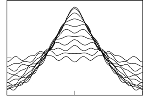
Figure 1. Two numerical solutions of (2.1) are shown at energy  $\mathscr {E}=0.4$. The free boundary, $y=\zeta (x)$, is shown for 11 values of time between $t=0$ and $t=0.25$, at which the maximal amplitude is reached. In (a), we have a gravity standing wave with $B=0$ and $F=0.3931$. In (b), we have a gravity-capillary standing wave with $B=0.003330$ and $F=0.4213$. These solutions were computed with $200$ spatial and $500$ temporal gridpoints, and here B and F are the Bond and Froude numbers defined in (2.2a,b).
For the related case of steadily travelling gravity-capillary waves (Stokes waves), it is known (e.g. Schwartz & Vanden-Broeck Reference Schwartz and Vanden-Broeck1979; Champneys, Vanden-Broeck & Lord Reference Champneys, Vanden-Broeck and Lord2002) that a small capillary effect results in a non-trivial bifurcation structure. Recently, it was demonstrated that as surface tension tends to zero, a continuum of solutions exists that exhibits highly oscillatory parasitic ripples (Shelton, Milewski & Trinh Reference Shelton, Milewski and Trinh2021; Shelton & Trinh Reference Shelton and Trinh2022). Thus, we might expect that time-dependent standing waves also exhibit this phenomena. However, we remark that oscillatory capillary ripples were not obviously present in the numerical standing-wave investigations of Schultz et al. (Reference Schultz, Vanden-Broeck, Jiang and Perlin1998), and this observation motivates the present study.
The purpose of this work is to show that these parasitic capillary ripples are, in fact, present in the time-dependent formulation of a standing gravity-capillary wave. An example solution containing these is shown in figure 1(b). Our results suggest that these features were not captured by Schultz et al. (Reference Schultz, Vanden-Broeck, Jiang and Perlin1998) due to their clustering of gridpoints about the wave crest, which resulted in an insufficient number across the rest of the spatial domain to resolve capillary ripples. We observe ripples that are highly oscillatory in space and time, and both respective frequencies are inversely proportional to the small surface tension parameter. When an amplitude condition (the wave energy) is fixed, a complicated bifurcation structure is seen to emerge. The branches of solutions are characterised by the wavenumber of the parasitic ripples, and along each branch, solutions transition from containing small-amplitude capillary ripples (such as that in figure 1b) to these ripples dominating the solution profile. This latter type is the nonlinear standing-wave analogue of the resonances found by Wilton (Reference Wilton1915) (cf. Appendix A). Given the already remarkable complexity of the pure gravity-driven standing waves (Wilkening Reference Wilkening2011), our results indicate that the inclusion of even a small amount of surface tension enhances the already rich dynamical structure of steep standing waves.
2. Mathematical formulation
We consider the time-dependent free-surface flow of a two-dimensional, inviscid, irrotational and incompressible fluid of infinite depth. Standing-wave solutions are sought, such that the free surface,  $\hat {\zeta }(\hat {x},\hat {t})$, and velocity potential, $\hat {\phi }(\hat {x},\hat {y},\hat {t})$ have temporal period $T$. We non-dimensionalise length scales by the wavelength $\lambda$, time by the physical interval $T$, and the velocity potential $\hat {\phi }$ by $\lambda ^2/T$. The non-dimensional governing equations then given by
 $$\begin{gather} \phi_{xx}+\phi_{yy}=0 \quad \text{for} \ y \leqslant \zeta, \end{gather}$$
 $$\begin{gather}\zeta_t=\phi_{y}-\zeta_{x}\phi_{x} \quad \text{at} \ y=\zeta, \end{gather}$$
 $$\begin{gather}F^2\phi_t+\frac{F^2}{2}(\phi^{2}_{x}+\phi^{2}_{y})+y-B\frac{\zeta_{xx}}{(1+\zeta_x^2)^{{3}/{2}}}=0 \quad \text{at}\ y=\zeta, \end{gather}$$
 $$\begin{gather}\phi_{x} \to 0 \quad \text{and} \quad \phi_{y} \to 0 \quad \text{as}\ y \to -\infty, \end{gather}$$
where the non-dimensional constants in Bernoulli's equation (2.1c),
 \begin{equation} F=\frac{\sqrt{\lambda}}{T\sqrt{g}} \quad \text{and} \quad B=\frac{\sigma}{\rho g \lambda^2}, \end{equation}
are the Froude and (inverse)-Bond numbers, respectively. The Froude number characterises the balance between inertia and gravity, and the Bond number characterises the balance between gravity and surface tension. Here,  $g$ is the gravitational constant, $\rho$ is the fluid density, $\sigma$ is the coefficient of surface tension, and $T$ and $\lambda$ are constants introduced from our choice of non-dimensionalisation. Note that if we instead had a wave speed $c=\lambda /T$ associated with steadily travelling waves, then our expression for the Froude number, $F$, in (2.2a) would be $F=c/\sqrt {g \lambda }$.
Furthermore, we enforce periodicity of the solutions in both time and space by enforcing
 $$\begin{gather} \boldsymbol{\nabla} \phi \left(x -1/2, y,t\right) = \boldsymbol{\nabla} \phi\left(x + 1/2, y,t\right), \quad \zeta\left(x - 1/2,t\right) = \zeta\left(x+1/2,t\right), \end{gather}$$
 $$\begin{gather}\boldsymbol{\nabla} \phi \left(x, y,0\right) = \boldsymbol{\nabla} \phi\left(x, y,1\right), \quad \zeta\left(x,0\right) = \zeta\left(x,1\right). \end{gather}$$
This results in a system with the two unknown constants,  $F$ and $B$. One of these will be fixed, and the other determined as an eigenvalue of the system through the imposition of an amplitude condition.
2.1. The time-dependent conformal mapping
The difficulty in computing numerical solutions to system (2.1) is that Bernoulli's equation (2.1c) holds along the unknown free surface,  $y=\zeta (x,t)$, which is also a function of time. In the study of steady flows, a well-established method is to invert the dependency of $\phi (x,y)$ and $\psi (x,y)$ to $x(\phi,\psi )$ and $y(\phi,\psi )$, for which the free surface, $\psi =0$, is parametrised by the velocity potential, $\phi$. However, in time-dependent flows, the constant value of the streamfunction, $\psi$, on the free surface will vary in time. To rectify this issue, we employ the time-dependent conformal mapping developed by Dyachenko, Zakharov & Kuznetsov (Reference Dyachenko, Zakharov and Kuznetsov1996) and Choi & Camassa (Reference Choi and Camassa1999), which maps the physical fluid domain $-\infty < y \leqslant \zeta (x,t)$ to the lower-half $(\xi,\eta )$-plane. Under this mapping, the free surface $y=\zeta (x,t)$ maps to the line $\eta =0$, for which the free-surface dynamics may be parametrised by $\xi$ and $t$. The following formulation closely follows that presented by Milewski, Vanden-Broeck & Wang (Reference Milewski, Vanden-Broeck and Wang2010).
We express the governing equations under the conformal mapping  $x=x(\xi,\eta,t)$ and $y=y(\xi,\eta,t)$. The free-surface variables, $Y$ and $\varPhi$, are defined by evaluating $y=\zeta (x,t)$ and $\phi (x,y,t)$ on $\eta =0$, yielding
 \begin{equation} Y(\xi,t)=\zeta(x(\xi,0,t),t) \quad \text{and} \quad \varPhi(\xi,t)=\phi(x(\xi,0,t),y(\xi,0,t),t). \end{equation}
Differentiation of (2.4a,b) with respect to  $\xi$ and $t$ yields equations that may be solved to obtain expressions for $\zeta _t$, $\phi _x$, $\phi _y$, $\zeta _x$ and $\zeta _{xx}$ in terms of these free-surface variables. Substitution of these resultant equations into the kinematic and dynamics boundary conditions (2.1b) and (2.1c) yields the following two time-evolution equations:
 $$\begin{gather} Y_t=Y_{\xi}\mathscr{H}\left[ \frac{\varPsi_{\xi}}{J}\right] - X_{\xi} \left( \frac{\varPsi_{\xi}}{J}\right), \end{gather}$$
 $$\begin{gather}\varPhi_t=\frac{1}{2}\left(\frac{\varPsi_{\xi}^2-\varPhi_{\xi}^2}{J}\right)+\varPhi_{\xi}\mathscr{H}\left[ \frac{\varPsi_{\xi}}{J}\right] -\frac{Y}{F^2}+\frac{B}{F^2}\frac{(X_{\xi}Y_{\xi\xi}-Y_{\xi}X_{\xi\xi})}{J^{3/2}}. \end{gather}$$
Here, we have defined the Jacobian of the mapping as  $J=X_{\xi }^2+Y_{\xi }^2$, and $\mathscr {H}$ is the periodic Hilbert transform defined later in (2.6). Additionally, expressions for $X(\xi,t)$ and $\varPsi (\xi,t)$ are known from the harmonic relations
 \begin{equation} X_{\xi}=1-\mathscr{H}[Y_{\xi}] \quad \text{and} \quad \varPsi_{\xi}=\mathscr{H}[\varPhi_{\xi}]. \end{equation}
The spatial and temporal periodicity conditions from (2.3) require that
 $$\begin{gather} \varPhi \left(\xi -1/2,t\right) = \varPhi\left(\xi + 1/2,t\right), \quad Y\left(\xi - 1/2,t\right) = Y\left(\xi+1/2,t\right), \end{gather}$$
 $$\begin{gather}\varPhi \left(\xi,0\right) = \varPhi\left(\xi,1\right), \quad Y\left(x,0\right) = Y\left(x,1\right), \end{gather}$$
and the amplitude condition is taken to be the energy
 \begin{equation} \mathscr{E}= \frac{1}{E_{hw}}\int_{{-}1/2}^{1/2} \Bigg[ \underbrace{\frac{F^2}{2} \varPsi\varPhi_{\xi}}_{\text{kinetic}}+\underbrace{\vphantom{\frac{1}{2}}B(J^{1/2}-X_{\xi})}_{\text{capillary}}+ \underbrace{\frac{1}{2} Y^2X_{\xi}}_{\text{gravitational}} \Bigg]{\rm d}{\xi}. \end{equation}
In the energy expression (2.5g), the three components are the kinetic energy, capillary potential energy and gravitational potential energy. We have also normalised with respect to  $E_{hw} = 0.00184$; this value is an approximation for the energy of the highest travelling Stokes wave, to three significant figures. We computed this value numerically in the present formulation with 4096 spatial gridpoints. It may also be found from table 2 of Longuet-Higgins (Reference Longuet-Higgins1975) which lists values of the kinetic and gravitational energies for different amplitudes, the sum of which is a factor of $4 {\rm \pi}^2$ larger than our current value. The Hilbert transform, required in the evaluation of (2.5a)–(2.5d) is given by
 \begin{equation} \mathscr{H}[Y](\xi) = \int_{-\infty}^{\infty} \frac{Y(\phi)}{\phi - \xi}\operatorname{d\!}{}{\phi} = \int_{{-}1/2}^{1/2} Y(\phi)\cot[{\rm \pi}(\phi - \xi)]\operatorname{d\!}{}{\phi}. \end{equation}
 System (2.5) consists of the two coupled time-evolution integro-differential equations for  $Y(\xi,t)$ and $\varPhi (\xi,t)$. Typically, we fix the Bond number, $B$, and the amplitude specified via the energy $\mathscr {E}$ in (2.5g). The unknown Froude number, $F$, is then determined as an eigenvalue. Occasionally, in order to numerically continue along solution branches, $\mathscr {E}$ and $F$ are fixed and $B$ is treated as the eigenvalue. Note that the energy (2.5g) is a conserved quantity (cf. (1.4) from Zakharov Reference Zakharov1968), and thus it may be evaluated at any point in time, unlike other ‘amplitude’ norms such as the wave crest-to-trough distance, or individual Fourier coefficients.
2.2. The numerical method
Rather than numerically compute solutions throughout the entire time interval  $0 \leqslant t \leqslant 1$, we use the symmetry remarked upon by Mercer & Roberts (Reference Mercer and Roberts1992) which requires only $0 \leqslant t \leqslant 1/4$. Provided that at $t=0$ the free surface, $Y$, is even and $\varPhi _{\xi }$ is odd about $\xi =0$ and at $t=1/4$ the fluid is at rest with $\varPhi _{\xi }=0$, at $t=1$ the solution will have returned to its initial state. These conditions are given formally by
 \begin{equation} Y(\xi,0)=Y(-\xi,0), \quad \varPhi_{\xi}(\xi,0)={-}\varPhi_{\xi}(-\xi,0), \quad \varPhi_{\xi}(\xi,1/4)=0. \end{equation}
We employ a shooting method to solve system (2.5) subject to conditions (2.7), in which we begin with an initial guess for the solutions  $Y$ and $\varPhi$ at $t=0$. This is evolved to $t=1/4$, at which point we seek to minimise each of conditions (2.7) and (2.5g) with Newton iteration. A detailed overview of this method is now provided.
(i) Initial guess. An initial guess for $Y(\xi,0)$, $\varPhi (\xi,0)$, and the eigenvalue (one of $B$ or $F$), is taken either from linear theory (Appendix A) or a previously computed solution. In discretising the spatial domain $\xi$ with $N$ grid points, such that $\xi _i=-1/2+i/N$ for $i=0, \ldots, N-1$, we define the solutions evaluated at each of these collocation points by $Y_i(t)=Y(\xi _i,t)$ and $\varPhi _i(t)=\varPhi (\xi _i,t)$. At $t=0$, $Y_i(0)$, $\varPhi _i(0)$ and the unknown eigenvalue yields a total of $2N+1$ unknowns.
(ii) Time evolution. We discretise the time interval
$t \in [0,1/4]$ into $M+1$ points, which yields $t_j=j/(4M)$ for $j=0,\ldots,M$. The fourth-order Runge–Kutta method is used to advance the solution from $t_j$ to $t_{j+1}$. With knowledge of $Y_i(t_j)$ and $\varPhi _i(t_j)$, the conjugate functions $X_i(t_j)$ and $\varPsi _i(t_j)$ are calculated from the harmonic relations (2.5c) and (2.5d). We use the Fourier transform to evaluate the derivatives and Hilbert transforms in (2.5a) and (2.5b). For instance, since the Fourier symbols for differentiation and the Hilbert transform are $2 {\rm \pi}\mathrm {i} k$ and $\mathrm {i}\ {\cdot }\ \text {sgn}(k)$, we have $Y_{\xi }=\mathscr {F}^{-1}[2 {\rm \pi}\mathrm {i} k \mathscr {F}[Y]]$ and $\mathscr {H}[Y]=\mathscr {F}^{-1}[\mathrm {i} {\cdot } \text {sgn}(k) \mathscr {F}[Y]]$, where $\mathscr {F}$ denotes the Fourier transform and k is the wavenumber. The fast Fourier transform algorithm is utilised to efficiently evaluate these identities. This allows for the calculation of the solutions $X_i(t_{j+1})$ and $\varPhi _i(t_{j+1})$ at the next time step. We de-alias by setting the highest $N/2$ Fourier modes to zero after nonlinearities are computed.(iii) Function to minimise. The previous step may be repeated until
$Y_i(1/4)$ and $\varPhi _i(1/4)$ are known. We then employ Newton iteration and the Levenberg–Marquardt algorithm on this system to minimise (2.5g) and (2.7) such that the square of the $l^2$-norm of the residual is below $10^{-10}$. This has been implemented in MATLAB with the inbuilt function fsolve. The even/odd conditions at $t=0$, (2.7a) and (2.7b), are evaluated in Fourier space where we require $\text {Im}[\mathscr {F}[Y]]=0$, and $\text {Re}[\mathscr {F}[\varPhi _{\xi }]]=0$.The symmetry condition (2.7a) on
$Y(\xi,0)$ gives $N/2$ equations; antisymmetry (2.7b) on $\varPhi _{\xi }(\xi,0)$ gives $N/2+1$ equations; the stationarity condition (2.7c), $\varPhi _{\xi }(\xi,1/4)=0$, gives $N$ equations; and the amplitude constraint (2.5g) gives $1$ equation. This formulation produces an overdetermined system with $2N+2$ equations and $2N+1$ unknowns.


For specified values of  $\mathscr {E}$ and $B$ for instance, this procedure yields a solution given by $Y(\xi,t)$, $\varPhi (\xi,t)$, and the eigenvalue $F$. In the sections that follow, we will plot $Y(X)$ by first calculating $X(\xi,t)=\xi -\mathscr {H}[Y]$.
3. Numerical results
3.1. Relationship to the study by Schultz et al. (Reference Schultz, Vanden-Broeck, Jiang and Perlin1998)
Numerical solutions of the standing gravity-capillary waves were calculated by Schultz et al. (Reference Schultz, Vanden-Broeck, Jiang and Perlin1998). They focused on large-amplitude solutions, and included capillary effects in order to compare with experimental wave profiles. However, their numerical solutions did not contain the parasitic ripples that we display in this section (see e.g. their figure 5). This is both because of the low number of spatial gridpoints they used (typically  $32$), as well as the clustering of such points near the wave crest to resolve the high curvature region.
Indeed Schultz et al. (Reference Schultz, Vanden-Broeck, Jiang and Perlin1998) were aware of this numerical limitation, as they had observed the formation of capillary ripples in the experimental profiles. They believed that these ripples were associated with resonances at certain values of the surface tension, and on p. 270 they commented that:
The ripple generation is related to the existence of multiple solutions of gravity-capillary waves at certain critical inverse Bond numbers [  $\ldots$]. The present calculation does not attempt to capture the solutions with these ripples $\ldots$ by using a small number of nodes to exclude the resonant superharmonics.
Here, we demonstrate that, while there are indeed solutions associated with resonances where the oscillatory ripples dominate the solution profile, the parasitic ripples are present throughout all solutions. Furthermore, the amplitude of non-resonant ripples increases with energy. Thus, the underresolved solutions determined by Schultz et al. (Reference Schultz, Vanden-Broeck, Jiang and Perlin1998) missed these ripples.
3.2. Structure of gravity-capillary standing waves
The numerical method described in § 2.2 is now implemented. We begin with a linear solution from Appendix A, which is used as a guess for our nonlinear solver when the energy is small. The energy is then increased over successive runs of Newton iteration, using a previously calculated numerical solution as an initial guess, until we reach a value of  $\mathscr {E}=0.4$. Numerical continuation is then used to explore the local branch structure at $\mathscr {E}=0.4$.
Figure 2 displays the resultant  $(B,F)$-bifurcation diagram from our investigations. Multiple branches are found, which appear to become self-similar as $B$ decreases. These standing-wave solutions, such as (a,b) from figure 3, are observed to contain small-amplitude parasitic capillary ripples, which are highly oscillatory in both space and time. These two solutions have $200$ gridpoints for $\xi \in [-1/2,1/2]$, $250$ in time for $t \in [0,1/4]$, and take approximately $5$ min on a desktop computer to be calculated. Each branch may be classified from the spatial wavenumber of the oscillatory ripples. This value differs by one between adjacent branches, increases as $B \to 0$, and may be confirmed to be of $O(1/B)$. The temporal wavenumber of the ripples also increases as $B \to 0$. This is shown in figure 4, in which the free surface at $x=-1/2$ is shown for $t \in [0,1/2]$ for solutions with different Bond numbers. The temporal wavenumber also differs by one between adjacent branches. Further, the amplitude of the ripples decreases as $B \to 0$, and the results in figure 5 suggest that this amplitude is exponentially small under this limit. It is interesting to note the similarity between the amplitudes shown in figure 5 and those in figure 5 of the exponential-asymptotic study by Shelton & Trinh (Reference Shelton and Trinh2023) for steadily travelling gravity-capillary waves.

Figure 2. The numerical bifurcation diagram of solutions is shown in the  $(B,F)$-plane for fixed energy, $\mathscr {E}=0.4$. Solutions (a–d) are displayed in figure 3 at $t=1/4$.

Figure 3. The free surface,  $y=\eta (x,t)$, is shown for 11 values of time in the interval $t \in [0,1/4]$ for the four solutions labelled in the bifurcation diagram of figure 2. Each profile has energy $\mathscr {E}=0.4$, and (a) $B=0.002830$ and $F=0.4171$, (b) $B=0.003650$ and $F=0.4240$, (c) $B=0.002846$ and $F=0.4158$, (d) $B=0.003206$ and $F=0.4190$.

Figure 4. The time evolution of the free surface at  $x=-1/2$, $y=\eta (1/2,t)$ is shown. This value of $x=-1/2$ corresponds to the wave trough in the solutions of figure 3. Note that to discern between each profile, we have vertically shifted the lower two by $-0.02$ and $-0.04$. It is seen that as the Bond number decreases, the temporal wavenumber of the parasitic ripples increases.

Figure 5. The amplitude of the parasitic capillary ripples present in the solution,  $y=\eta (x,t)$, is shown at $t=1/4$. Multiple capillary ripple amplitudes are shown, corresponding to solutions across each branch of figure 2 with energy $\mathscr {E}=0.4$. To measure the amplitude of this high-frequency component, lower modes have been filtered out in Fourier space.
As each of the branches of solutions is continued, the capillary ripple amplitude increases. Example solutions are shown profiles (c,d) of figure 3. More Fourier coefficients were required to determine these. We used  $400$ spatial gridpoints and $1250$ time steps, for which each solution took approximately $60$ min to determine. We note that while these solutions still satisfy the same bound on the residual of $10^{-10}$, the decay of the Fourier modes is unsatisfactory. This is shown in figure 6(b), in which the Fourier coefficient decay at $t=1/4$ is compared between solutions (a,d) from figure 3. This poor decay for solution (d) may be in part due to the conformal map formulation, which distributes gridpoints away from high-curvature regions. For most solutions in figure 2 this has not been an issue, which may be confirmed from the Fourier coefficient decay in figure 6(b). In figure 6(a), we plot each component of the energy (2.5g) across $t \in [0,1/4]$ for the same two solutions, (a,d) in figure 3. The solution near the end of the computed branch (solid marks) has more capillary and kinetic energy than that in the middle of the branch (hollow marks). As the fluid is at rest at $t=1/4$, when the wave reaches its maximal amplitude, the kinetic energy is zero. We anticipate that the adjacent branches in figure 2 connect via solutions whose fundamental wavelengths (in both space and time) are smaller than unity. These solutions would be purely oscillatory, which is analogous to the bifurcation diagram from Shelton et al. (Reference Shelton, Milewski and Trinh2021), but our present numerical formulation is unable to resolve this regime in practice.

Figure 6. (a) Each component of the solution energy (2.5g) is shown throughout the time period. (b) The magnitude of the Fourier coefficients is shown at  $t=1/4$, when the standing wave reaches its maximum height. These are shown for the two solutions (a,d) from figure 3, where solid corresponds to solution (a) and hollow to (d).
4. Conclusions
We have numerically demonstrated that for small surface tension, gravity-capillary standing waves contain parasitic capillary ripples, which are highly oscillatory in both space and time. These ripples, for which the spatial and temporal wavenumbers are both of  $O(1/B)$, result in a discrete set of solution branches existing in the limit of $B \to 0$. As each branch is traversed in the direction of decreasing surface tension, the oscillatory capillary ripples transition from $n$ to $n+1$ periods (in both space and time). The amplitude of these ripples is observed to be predominantly exponentially small in the surface tension parameter, $B$, but rapidly increases when approaching the numerical endpoints of each computed branch; the computational difficulty increases dramatically as these points are approached, and our numerical algorithm is unable to resolve any further. To resolve the bifurcation structure, we have implemented a numerical scheme that is capable of solving for steep standing waves, and also has a sufficient number of gridpoints distributed across the domain.
We conjecture that the discrete solution branches will connect to one another, and that this occurs when the fundamental wavelengths (in both space and time) of the solution are both smaller than one. These purely oscillatory solutions would be similar to those observed in the steadily travelling bifurcation diagram by Shelton et al. (Reference Shelton, Milewski and Trinh2021). However, on the account of the challenging computations, the numerical formulation needed to verify this is still lacking.
5. Discussion
In this work, we have focused on gravity-capillary standing waves in the small surface tension limit of  $B \to 0$. The question of the full global structure of the ( $B, F, \mathscr {E}$) bifurcation diagram is fascinating. As demonstrated by Wilkening (Reference Wilkening2011) for highly nonlinear standing gravity waves, solutions exhibit a remarkably complex set of dynamics, each distinguished by varying oscillations near the crest. Our work here also demonstrates complicated behaviour for small surface tension. However, the $B \to 0$ limit contains structure that can perhaps be exploited in the future by exponential-asymptotic methods.
5.1. Temporally periodic travelling gravity-capillary waves
It was shown numerically by Wilkening (Reference Wilkening2021) that a continuous solution branch exists between travelling and standing gravity waves. Intermediate states are solutions which periodically repeat in time together with a shift in space. This travelling/standing connection may be investigated in our present gravity-capillary formulation, for which the bifurcation structure uncovered here could be connected to that of steadily travelling waves from Shelton et al. (Reference Shelton, Milewski and Trinh2021) which have similar structure.
It is unknown whether nonlinear travelling solutions exist with non-trivial temporal periodicity. Asymptotically as  $B \to 0$, these solutions could correspond to unsteady capillary ripples appearing as a perturbation to a leading-order steadily travelling gravity wave. These solutions were conjectured to exist by Jervis (Reference Jervis1996). Subsequent numerical studies by e.g. Jiang et al. (Reference Jiang, Lin, Schultz and Perlin1999) and Murashige & Choi (Reference Murashige and Choi2017) have investigated a closely related time-evolution problem with an initial condition of a steadily travelling gravity wave, where surface tension is switched on for $t>0$. In these works, unsteady parasitic ripples are observed to form, but no condition on temporal periodicity is enforced.
5.2. Beyond-all-order asymptotics of nonlinear partial differential equations
In the perturbative study by Shelton & Trinh (Reference Shelton and Trinh2022), analytical solutions were found for the parasitic capillary ripples present on steep travelling gravity waves using beyond-all-order asymptotics. Since these solutions are steady in the co-moving frame, they are governed by nonlinear integro-differential equations with just one independent variable – this is opposed to our current formulation where solutions depends on both  $\xi$ and $t$. Many unresolved complications arise, however, in exponential asymptotics for nonlinear partial differential equations (Howls, Langman & Olde Daalhuis Reference Howls, Langman and Olde Daalhuis2004; Body, King & Tew Reference Body, King and Tew2005; Chapman & Mortimer Reference Chapman and Mortimer2005), and the beyond-all-orders analysis of such problems is an exciting area of future research.
Acknowledgements
We thank Professor J. Toland (Bath) for a number of useful and interesting discussions on the challenges of the Penney–Price (gravity standing-wave) problem. We also thank the anonymous reviewers for their suggestions that improved the clarity of our work.
Funding
J.S. and P.H.T. acknowledge support by the Engineering and Physical Sciences Research Council (EPSRC grant no. EP/V012479/1). J.S. is additionally supported by the Engineering and Physical Sciences Research Council (EPSRC grant no. EP/W522491/1).
Declaration of interests
The authors report no conflict of interest.
Appendix A. Linear theory for standing waves
We consider the first two terms of a Stokes expansion by writing  $Y=Y_0+\epsilon Y_1$, $X=X_0+\epsilon X_1$, $\varPhi =\varPhi _0+\epsilon \varPhi _1$ and $\varPsi =\varPsi _0+\epsilon \varPsi _1$. At $O(\epsilon ^0)$ in (2.5a) to (2.5d), we find the solutions $Y_0=0$, $X_0=\xi$, $\varPhi _0=0$ and $\varPsi _0=0$. Next, at $O(\epsilon )$ we have the equations
 \begin{equation} Y_{1t}={-}\mathscr{H}[\varPhi_{1 \xi}] \quad \text{and} \quad F^2 \varPhi_{1t}={-}Y_1 +BY_{1 \xi \xi}. \end{equation}
In writing the solutions as a Fourier series of the form
 \begin{equation} Y_1(\xi,t)=a_0(t)+\sum_{k=1}^{\infty} \left[a_k(t)\cos{(2k {\rm \pi}\xi)} +b_k(t)\sin(2 k {\rm \pi}\xi)\right], \end{equation}
with a similar expansion for  $\varPhi _1(\xi,t)$ in terms of the Fourier coefficients $c_k(t)$ and $d_k(t)$, we find for $k \geqslant 1$ the two second-order differential equations
 \begin{equation} \left(\begin{matrix} a_k^{\prime \prime}(t)\\ b_k^{\prime \prime}(t) \end{matrix} \right)={-}\frac{2k {\rm \pi}}{F^2} \left(1+(2k {\rm \pi})^2B\right) \left(\begin{matrix} a_k(t)\\ b_k(t) \end{matrix} \right). \end{equation}
Note that we necessarily have  $a_0(t)=0$ in order for the $k=0$ mode in $\varPhi _1(\xi,t)$ to be temporally periodic.
We now express the solutions to (A3) as a Fourier series in time of the form
 \begin{equation} a_k(t)=\hat{a}^{(k)}_0+\sum_{m=1}^{\infty} \left[\hat{a}_m^{(k)}\cos{(2 m {\rm \pi}t)} +\bar{a}_m^{(k)}\sin(2 m {\rm \pi}t)\right], \end{equation}
with a similar expansion for  $b_k(t)$ in terms of the Fourier coefficients $\hat {b}_m^{(k)}$ and $\bar {b}_m^{(k)}$. Substitution of (A4) into the differential equation (A3) yields the dispersion relation
 \begin{equation} F^2 - \frac{k}{2 {\rm \pi}m^2} \left(1+(2k {\rm \pi})^2B \right)=0. \end{equation}
Here,  $k\geqslant 1$ is the spatial mode, and $m \geqslant 1$ is the temporal mode. Note that if $m=k$, (A5) reduces to the steady dispersion relation for gravity-capillary waves. When (A5) is satisfied, a non-zero $m$th mode in the Fourier series expansions for $a_k(t)$ and $b_k(t)$ is permitted. Furthermore, the symmetry condition (2.5e) for $Y(\xi,0)$ requires that $\hat {b}_m^{(k)}=0$. Asymmetry on $\varPhi (\xi,0)$, through the equation $a_k^{\prime }(t)=2 k {\rm \pi}c_k(t)$, yields $\bar {a}_m^{(k)}=0$. This gives a linear solution of the form
 \begin{equation} \left.\begin{gathered} Y_1(\xi,t)= \hat{a}_m^{(k)}\cos{(2m {\rm \pi}t)} \cos{(2k {\rm \pi}\xi)}+ \bar{b}_m^{(k)}\sin{(2m {\rm \pi}t)} \sin{(2k {\rm \pi}\xi)},\\ \varPhi_1(\xi,t)={-}\frac{m\hat{a}_m^{(k)}}{k}\sin{(2m {\rm \pi}t)} \cos{(2k {\rm \pi}\xi)}+ \frac{m\bar{b}_m^{(k)}}{k}\cos{(2m {\rm \pi}t)} \sin{(2k {\rm \pi}\xi)}.\end{gathered}\right\} \end{equation}
 Multiple Fourier modes may be non-zero in the solution if the linear dispersion relation (A5) is satisfied for two values of  $k=\{k_1,k_2\}$ and $m=\{m_1,m_2\}$. This yields
 \begin{equation} B=\frac{1}{4 {\rm \pi}^2} \left(\frac{m_1^2k_2-m_2^2k_1}{m_2^2k_1^3-m_1^2k_2^3}\right) \quad \text{and} \quad F^2=\frac{1}{2 {\rm \pi}} \left(\frac{k_1 k_2(k_1+k_2)(k_1-k_2)}{m_2^2k_1^3-m_1^2k_2^3}\right), \end{equation}
which reduces to the steadily travelling  $(1,k)$ resonance found by Wilton (Reference Wilton1915) when $m_1=k_1$ and $m_2=1=k_2$.


 Open access