


1 Introduction
Let $g,h,N$
be positive integers. A subset
$g,h,N$
be positive integers. A subset $A \subset [N] = \{1,2,\ldots ,N\}$
is a
$A \subset [N] = \{1,2,\ldots ,N\}$
is a $B_h[g]$
set if, for every
$B_h[g]$
set if, for every $x \in \mathbb {Z}$
, there are at most g representations of the form
$x \in \mathbb {Z}$
, there are at most g representations of the form
 $$\begin{align*}a_1 + a_2 + \cdots + a_h = x, \quad a_i \in A, \quad 1 \leq i \leq h, \end{align*}$$
where two representations are considered to be the same if they are permutations of each other. As a shorthand, we let $B_h = B_h[1]$
. Note that
$B_h = B_h[1]$
. Note that $B_2$
sets are the very well-known Sidon sets. Let
$B_2$
sets are the very well-known Sidon sets. Let $R_h[g](N)$
denote the largest size of subset
$R_h[g](N)$
denote the largest size of subset $A \subset [N]$
such that A is a
$A \subset [N]$
such that A is a $B_h[g]$
set. By counting the number of ordered h-tuples of elements of A, we have the simple bound
$B_h[g]$
set. By counting the number of ordered h-tuples of elements of A, we have the simple bound $\binom {|A|+h-1}{h} \leq ghN$
, which implies
$\binom {|A|+h-1}{h} \leq ghN$
, which implies $R_h[g](N) \leq (ghh!N)^{1/h}$
. On the other hand, Bose and Chowla showed that there exist
$R_h[g](N) \leq (ghh!N)^{1/h}$
. On the other hand, Bose and Chowla showed that there exist $B_h$
sets of size
$B_h$
sets of size $N^{1/h}(1+o(1))$
, where we use
$N^{1/h}(1+o(1))$
, where we use $o(1)$
to denote a term going to zero as
$o(1)$
to denote a term going to zero as $N \to \infty $
[Reference Bose and Chowla2]. This lower bound result has been generalized to more pairs
$N \to \infty $
[Reference Bose and Chowla2]. This lower bound result has been generalized to more pairs $(g,h)$
by several authors [Reference Caicedo, Gómez and Trujillo3, Reference Cilleruelo and Jiménez-Urroz4, Reference Lindström11]. Recently, the bound
$(g,h)$
by several authors [Reference Caicedo, Gómez and Trujillo3, Reference Cilleruelo and Jiménez-Urroz4, Reference Lindström11]. Recently, the bound $R_h[g](N) \geq (Ng)^{1/h}(1-o(1))$
for all N,
$R_h[g](N) \geq (Ng)^{1/h}(1-o(1))$
for all N, $g \geq 1$
, and
$g \geq 1$
, and $h\geq 2$
was obtained in [Reference Johnston, Tait and Timmons10]. In general, estimating the constant
$h\geq 2$
was obtained in [Reference Johnston, Tait and Timmons10]. In general, estimating the constant
 $$\begin{align*}\sigma_h(g) = \lim_{N \to \infty} \frac{R_h[g](N)}{(gN)^{1/h}} \end{align*}$$
is an open problem. In fact, the only case for which the above limit is known to exist is in the case of the classical Sidon sets, where we have $\sigma _2(1) = 1$
. Henceforth, we will understand upper and lower bounds on
$\sigma _2(1) = 1$
. Henceforth, we will understand upper and lower bounds on $\sigma _h(g)$
to be estimates on the
$\sigma _h(g)$
to be estimates on the $\limsup $
and
$\limsup $
and $\liminf $
, respectively.
$\liminf $
, respectively.
Several improved upper bounds for $\sigma _h(g)$
have been obtained by various authors, for references to many of them, as well as an excellent resource on
$\sigma _h(g)$
have been obtained by various authors, for references to many of them, as well as an excellent resource on $B_h[g]$
sets in general (see [Reference O’Bryant16]). In this work, we will improve the upper bounds on
$B_h[g]$
sets in general (see [Reference O’Bryant16]). In this work, we will improve the upper bounds on $\sigma _h(g)$
for
$\sigma _h(g)$
for $h = 2$
and
$h = 2$
and $2 \leq g \leq 4$
, as well as
$2 \leq g \leq 4$
, as well as $g = 1$
and
$g = 1$
and $h = 3,4$
. No improvement on
$h = 3,4$
. No improvement on $\sigma _h(g)$
for
$\sigma _h(g)$
for $g = 1$
and
$g = 1$
and $h=3,4$
has been made since [Reference Green7] in 2001. The most recent improvements on estimates for
$h=3,4$
has been made since [Reference Green7] in 2001. The most recent improvements on estimates for $\sigma _2(g)$
which are the best for
$\sigma _2(g)$
which are the best for $2 \leq g \leq 4$
are the following:
$2 \leq g \leq 4$
are the following:
 $$ \begin{align*} \sigma_2(g) & \leq \sqrt{1.75(2-1/g)} & \text{Green } [7]\\ & \leq \sqrt{1.74217(2-1/g)} & \text{Yu } [18]\\ & \leq \sqrt{1.740463(2-1/g)}. & \text{Habsieger and Plagne } [9] \end{align*} $$
On the other hand, for $g \geq 5$
, the best recent upper bounds are the following:
$g \geq 5$
, the best recent upper bounds are the following:
 $$ \begin{align*} \sigma_2(g) & \leq \sqrt{3.4796} & \text{Cilleruelo, Ruzsa and Trujillo } [5] \\ & \leq \sqrt{3.1696} & \text{Martin and O'Bryant } [13]\\ & \leq \sqrt{3.1377} & \text{Matolcsi and Vinuesa } [15]\\ & \leq \sqrt{3.1250}. & \text{Cloninger and Steinerberger } [6] \end{align*} $$
Interestingly, the key to improving upper bounds on $\sigma _2(g)$
is to better estimate the 2-norm of an autoconvolution for small g and the infinity norm of an autoconvolution for large g. In the case of the infinity norm, the best-known results are
$\sigma _2(g)$
is to better estimate the 2-norm of an autoconvolution for small g and the infinity norm of an autoconvolution for large g. In the case of the infinity norm, the best-known results are
 $$\begin{align*}0.64 \leq \inf_{\substack{f \colon [-1/2,1/2] \to \mathbb{R}_{\geq 0} \\ \int f \ = \ 1}} \| f \ast f\|_\infty \leq 0.75496. \end{align*}$$
The lower bound is due to Cloninger and Steinerberger [Reference Cloninger and Steinerberger6], and the upper bound is due to Matolcsi and Vinuesa [Reference Matolcsi and Vinuesa15]. It is believed that the upper bound above is closer to the truth. The method of Cloninger and Steinerberger is computational, and is limited by a nonconvex optimization program.
Throughout, we denote by $\mathcal {F}$
the family of nonnegative functions
$\mathcal {F}$
the family of nonnegative functions $f \in L^1(-1/2,1/2)$
such that
$f \in L^1(-1/2,1/2)$
such that $\int f = 1$
. For
$\int f = 1$
. For $1 \leq p \leq \infty $
, we define
$1 \leq p \leq \infty $
, we define
 $$\begin{align*}\mu_p = \inf_{f \in \mathcal{F}} \| f \ast f \|_p =\inf_{f \in \mathcal{F}}\left( \int_{-1}^1 \left( \int_{-1/2}^{1/2} f(t)f(x-t) dt \right)^p dx\right)^{1/p} ,\end{align*}$$
the minimum p-norm of the autoconvolution supported on a unit interval. Determining $\mu _p$
precisely is an open problem for all values of p, and is the content of Problem 35 in Ben Green’s 100 open problems [Reference Green8]. Prior to this work, the best-known bounds for the
$\mu _p$
precisely is an open problem for all values of p, and is the content of Problem 35 in Ben Green’s 100 open problems [Reference Green8]. Prior to this work, the best-known bounds for the $p = 2$
case are
$p = 2$
case are
 $$\begin{align*}0.574575 \leq \mu_2^2 \leq 0.640733,\end{align*}$$
where the lower bound is due to Martin and O’Bryant [Reference Martin and O’Bryant14] and the upper bound is due to Green [Reference Green7]. Our main theorem is the following, and we improve upper and lower bounds for $\mu _2$
.
$\mu _2$
.
Theorem 1.1 The infimum of the $L^2$
-norm of an autoconvolution
$L^2$
-norm of an autoconvolution $f \ast f$
for
$f \ast f$
for $f \in \mathcal {F}$
can be bounded as follows:
$f \in \mathcal {F}$
can be bounded as follows:
 $$\begin{align*}\mathbf{0.5746}36066 \leq \mu_2^2 \leq \mathbf{0.5746}42912. \end{align*}$$
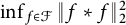
We are also able to prove that there exists a unique minimizer $f \in \mathcal {F}$
of the
$f \in \mathcal {F}$
of the $L^2$
-norm of an autoconvolution. Our method produces arbitrarily close approximations to the minimizer. The function
$L^2$
-norm of an autoconvolution. Our method produces arbitrarily close approximations to the minimizer. The function $f \in \mathcal {F}$
with the smallest
$f \in \mathcal {F}$
with the smallest $L^2$
-norm of its autoconvolution we computed is shown in Figure 1. We also show its autoconvolution
$L^2$
-norm of its autoconvolution we computed is shown in Figure 1. We also show its autoconvolution $f \ast f$
, and the function
$f \ast f$
, and the function $\pi f(x)\sqrt {1/4-x^2}$
. Notably, the function
$\pi f(x)\sqrt {1/4-x^2}$
. Notably, the function $\pi f(x)\sqrt {1/4-x^2}$
takes values in
$\pi f(x)\sqrt {1/4-x^2}$
takes values in $[0.99,1.02]$
for
$[0.99,1.02]$
for $|x| \leq 0.499$
. A singularity of strength
$|x| \leq 0.499$
. A singularity of strength $1/\sqrt {x}$
at the boundary of the
$1/\sqrt {x}$
at the boundary of the $[-1/2,1/2]$
domain creates an autoconvolution that neither vanishes nor “blows up” at the boundary, as demonstrated by
$[-1/2,1/2]$
domain creates an autoconvolution that neither vanishes nor “blows up” at the boundary, as demonstrated by $f \ast f$
. Similar functions were studied by Barnard in Steinerberger on their work on convolution inequalities [Reference Barnard and Steinerberger1].
$f \ast f$
. Similar functions were studied by Barnard in Steinerberger on their work on convolution inequalities [Reference Barnard and Steinerberger1].

Figure 1 A close approximation to the minimizer.
Combining our new bounds on $\mu _2^2$
with methods of Green [Reference Green7, Theorems 15, 17, and 24] gives the following corollary.
$\mu _2^2$
with methods of Green [Reference Green7, Theorems 15, 17, and 24] gives the following corollary.
Corollary 1.2 The following asymptotic bounds on $B_h[g]$
sets hold:
$B_h[g]$
sets hold:
 $$\begin{align*}\sigma_2(g) \leq \left(\frac{2-1/g}{\underline{\mu_2^2}}\right)^{1/2} ,\quad \sigma_3(1) \leq \left(\frac{2}{\underline{\mu_2^2}} \right)^{1/3}, \quad\sigma_4(1) \leq \left(\frac{4}{\underline{\mu_2^2}} \right)^{1/4}, \end{align*}$$
where $\underline {\mu _2^2} = 0.574636066$
denotes the lower bound on
$\underline {\mu _2^2} = 0.574636066$
denotes the lower bound on $\mu _2^2$
stated in Theorem 1.1.
$\mu _2^2$
stated in Theorem 1.1.
Corollary 1.2 is an improvement on the previous best upper bounds for $\sigma _h[g]$
for
$\sigma _h[g]$
for $h=2$
and
$h=2$
and $2 \leq g \leq 4$
as well as
$2 \leq g \leq 4$
as well as $g = 1$
and
$g = 1$
and $h = 3,4$
. One of the main theorems proved by Green in [Reference Green7] gives a bound on the additive energy of a discrete function on
$h = 3,4$
. One of the main theorems proved by Green in [Reference Green7] gives a bound on the additive energy of a discrete function on $[N]$
. We show that our bound in the continuous case applies to the discrete one, and so the Theorem 1.1 bound gives another improved estimate.
$[N]$
. We show that our bound in the continuous case applies to the discrete one, and so the Theorem 1.1 bound gives another improved estimate.
Corollary 1.3 Let $H \colon [N] \to \mathbb {R}_{\geq 0}$
be a function with
$H \colon [N] \to \mathbb {R}_{\geq 0}$
be a function with $\sum _{j=1}^N H(j) = N$
. Then, for all sufficiently large N, we have
$\sum _{j=1}^N H(j) = N$
. Then, for all sufficiently large N, we have
 $$\begin{align*}\sum_{a+b = c+d} H(a)H(b)H(c)H(d) \geq \mu_2^2 N^3. \end{align*}$$
The methods of Habsieger, Plagne, and Yu [Reference Habsieger and Plagne9, Reference Yu18], Cloninger and Steinerberger [Reference Cloninger and Steinerberger6], and Martin and O’Bryant are all limited by long computation times. In contrast, the key to our improvement is a convex quadratic optimization program whose optimum value is shown to converge to $\mu _2^2$
. The strategy of using Fourier analysis to produce a convex program to obtain bounds on a convolution-type inequality was also employed recently by the author to improve bounds on Erdős’ minimum overlap problem in [Reference White17]. We hope that our methods may also be useful in obtaining estimates for the infimum of an autoconvolution with respect to other p-norms.
$\mu _2^2$
. The strategy of using Fourier analysis to produce a convex program to obtain bounds on a convolution-type inequality was also employed recently by the author to improve bounds on Erdős’ minimum overlap problem in [Reference White17]. We hope that our methods may also be useful in obtaining estimates for the infimum of an autoconvolution with respect to other p-norms.
2 Existence and uniqueness of the optimizer
In this section, we prove the existence and uniqueness to the solution of the following optimization problem:
 $$ \begin{align} \text{Infimum:} & \int_{-1}^{1} (f \ast f)^2(x) \ dx, \end{align} $$
 $$ \begin{align} \text{Such that: }& f \colon [-1/2,1/2] \to \mathbb{R}_{\geq 0} \quad \int_{-1/2}^{1/2} f(x) \ dx = 1. \end{align} $$
We remark that (2.2) defines the family $\mathcal {F}$
seen in the introduction. For all
$\mathcal {F}$
seen in the introduction. For all $f \in L^1(\mathbb {R})$
, we define the Fourier transform on
$f \in L^1(\mathbb {R})$
, we define the Fourier transform on $\mathbb {R}$
as
$\mathbb {R}$
as
 $$\begin{align*}\tilde{f}(y) = \int_{\mathbb{R}} e^{-2\pi i xy}f(x) \ dx.\end{align*}$$
For any f as in (2.2), we note that $\widetilde {f \ast f} = \tilde {f}^2$
, and so by Parseval’s identity,
$\widetilde {f \ast f} = \tilde {f}^2$
, and so by Parseval’s identity,
 $$ \begin{align} \int_{-1}^{1} (f \ast f)^2(x) \ dx = \int_{\mathbb{R}} |\tilde{f}(y)|^4 \ dy. \end{align} $$
The following proposition proves the existence and uniqueness of an optimizer in $\mathcal {F}$
to (2.1) using the “direct method in the calculus of variations.” A similar method is used to show the existence of optimizers to autocorrelation inequalities in [Reference Madrid and Ramos12].
$\mathcal {F}$
to (2.1) using the “direct method in the calculus of variations.” A similar method is used to show the existence of optimizers to autocorrelation inequalities in [Reference Madrid and Ramos12].
Proposition There exists a unique extremizing function $f \in \mathcal {F}$
to the optimization problem (2.1).
$f \in \mathcal {F}$
to the optimization problem (2.1).
Proof Let $\{f_n\} \subset \mathcal {F}$
be a minimizing sequence such that
$\{f_n\} \subset \mathcal {F}$
be a minimizing sequence such that ${\lim _{n \to \infty } \| f_n \ast f_n \|_2 = \mu _2}$
. Since
${\lim _{n \to \infty } \| f_n \ast f_n \|_2 = \mu _2}$
. Since $L^1$
and
$L^1$
and $L^\infty $
are separable, we can apply the sequential Banach–Alaoglu theorem to conclude the existence of
$L^\infty $
are separable, we can apply the sequential Banach–Alaoglu theorem to conclude the existence of $f \in L^{1}(-1/2,1/2)$
and
$f \in L^{1}(-1/2,1/2)$
and $g \in L^\infty (\mathbb {R})$
such that
$g \in L^\infty (\mathbb {R})$
such that
 $$ \begin{align*} f_n &\stackrel{\ast}{\rightharpoonup} f & \text{converges weakly in } L^{1}(-1/2,1/2), \\ \tilde{f_n} &\stackrel{\ast}{\rightharpoonup} g & \text{converges weakly in } L^{\infty}(\mathbb{R}), \end{align*} $$
where possibly we passed to a subsequence of $\{f_n\}$
to make the above hold. For all
$\{f_n\}$
to make the above hold. For all $h \in L^{1}(\mathbb {R})$
, by definition of convergence in the weak topology, we have
$h \in L^{1}(\mathbb {R})$
, by definition of convergence in the weak topology, we have
 $$\begin{align*}\langle g,h \rangle = \lim_{n \to \infty} \langle \tilde{f}_n ,h \rangle = \lim_{n \to \infty} \langle {f}_n ,\tilde{h} \rangle = \langle {f} , \tilde{h} \rangle= \langle \tilde{f} , h \rangle; \end{align*}$$
hence $g = \tilde {f}$
. Note that for all
$g = \tilde {f}$
. Note that for all $y \in \mathbb {R}$
, we have
$y \in \mathbb {R}$
, we have
 $$\begin{align*}\tilde{f_n}(y) = \int_{\mathbb{R}} f_n(x)e^{-2\pi i x y} \mathbf{1}_{(-1/2,1/2)}(x) \ dx, \end{align*}$$
and since $e^{-2\pi i x y} \mathbf {1}_{(-1/2,1/2)}(x) \in L^\infty (\mathbb {R})$
, by weak convergence, we see
$e^{-2\pi i x y} \mathbf {1}_{(-1/2,1/2)}(x) \in L^\infty (\mathbb {R})$
, by weak convergence, we see $\lim _{n \to \infty } \tilde {f_n}(y) = \tilde {f}(y)$
. In addition,
$\lim _{n \to \infty } \tilde {f_n}(y) = \tilde {f}(y)$
. In addition, $\lim _{n \to \infty } |\tilde {f_n}(y)|^4 = |\tilde {f}(y)|^4$
, and so by Fatou’s lemma,
$\lim _{n \to \infty } |\tilde {f_n}(y)|^4 = |\tilde {f}(y)|^4$
, and so by Fatou’s lemma,
 $$\begin{align*}\int_{\mathbb{R}} |\tilde{f}(y)|^4 \ dy \leq \liminf_{n \to \infty} \int_{\mathbb{R}} |\tilde{f_n}(y)|^4\ \ dy .\end{align*}$$
Finally, we have
 $$\begin{align*}1 = \lim_{n \to \infty} \langle \mathbf{1}_{(-1/2,1/2)}, f_n \rangle = \langle \mathbf{1}_{(-1/2,1/2)},f \rangle = \int_{-1/2}^{1/2} f(x) \ dx.\end{align*}$$
We conclude that $f \in \mathcal {F}$
is an extremizing function. For uniqueness, suppose that
$f \in \mathcal {F}$
is an extremizing function. For uniqueness, suppose that $f,g \in \mathcal {F}$
satisfy
$f,g \in \mathcal {F}$
satisfy $\|\tilde {f}\|_4 = \| \tilde {g}\|_4 = \mu _2^{1/2}$
. Then, by Minkowski’s inequality,
$\|\tilde {f}\|_4 = \| \tilde {g}\|_4 = \mu _2^{1/2}$
. Then, by Minkowski’s inequality,
 $$\begin{align*}\left\| \frac{\tilde{f} + \tilde{g}}{2} \right\|_4 \leq \frac{1}{2} \left( \|\tilde{f} \|_4 + \|\tilde{g}\|_4 \right) = \mu_2^{1/2}.\end{align*}$$
Minkowski’s inequality above must be an equality, implying f and g are linearly dependant. Since $f,g$
have the same average value, we conclude that
$f,g$
have the same average value, we conclude that $f = g$
and so the extremizing function is unique.
$f = g$
and so the extremizing function is unique.
Note that the uniqueness of the optimizer implies that it must be even. Throughout, we will denote the unique optimizer by $f^\Diamond \in \mathcal {F}$
.
$f^\Diamond \in \mathcal {F}$
.
3 Useful identities
For ease of notation, we will always use lowercase letters $f,g$
to denote functions on
$f,g$
to denote functions on $[-1/2,1/2]$
, or period 1 functions. We define the Fourier transform of
$[-1/2,1/2]$
, or period 1 functions. We define the Fourier transform of $f \colon [-1/2,1/2] \to \mathbb {R}$
for
$f \colon [-1/2,1/2] \to \mathbb {R}$
for $k \in \mathbb {Z}$
as
$k \in \mathbb {Z}$
as
 $$\begin{align*}\hat{f}(k) = \int_{-1/2}^{1/2} e^{-2\pi i k x} f(x) \ dx. \end{align*}$$
We will use upper case letters $F,G$
to denote functions on
$F,G$
to denote functions on $[-1,1]$
or period 2 functions. We define the Fourier transform of
$[-1,1]$
or period 2 functions. We define the Fourier transform of $F \colon [-1,1] \to \mathbb {R}$
for
$F \colon [-1,1] \to \mathbb {R}$
for $k \in \mathbb {Z}$
as
$k \in \mathbb {Z}$
as
 $$\begin{align*}\hat{F}(k) = \frac{1}{2}\int_{-1}^{1} e^{-\pi i k x} f(x) \ dx. \end{align*}$$
This is an abuse of the notation “ $\hat {}$
,” but which of the two above transforms is meant will be made clear by the letter case of the function notation. Let
$\hat {}$
,” but which of the two above transforms is meant will be made clear by the letter case of the function notation. Let $f \in \mathcal {F}$
and define
$f \in \mathcal {F}$
and define $F(x)$
be the extension of
$F(x)$
be the extension of $f(x)$
to a function on
$f(x)$
to a function on $[-1,1]$
defined by setting
$[-1,1]$
defined by setting $F(x)= 0$
outside of
$F(x)= 0$
outside of $[-1/2,1/2]$
. Since
$[-1/2,1/2]$
. Since $\text {supp}(F) \subset [-1/2,1/2]$
, the support of
$\text {supp}(F) \subset [-1/2,1/2]$
, the support of $F \ast F$
is contained in
$F \ast F$
is contained in $[-1,1]$
; hence,
$[-1,1]$
; hence,
 $$\begin{align*}\widehat{F\ast F}(k) = \frac{1}{2} \int_{-1}^1 e^{-\pi i kx}F\ast F(x) \ dx = \frac{1}{2} \int_{-1}^1 e^{-\pi i kx}\int_{-1/2}^{1/2} f(t)f(x-t) \ dt \ dx \end{align*}$$
 $$ \begin{align*} \quad=\frac{1}{2} \int_{-1/2}^{1/2} e^{-\pi i k t} F(t) \int_{-1}^1 e^{-\pi i k(x-t)}F(x-t) \ dx \ dt = 2 \hat{F}(k)^2. \end{align*} $$
We calculate the relationship between $\hat {F}$
and
$\hat {F}$
and $\hat {f}$
below:
$\hat {f}$
below:
 $$ \begin{align} \hat{F}(m) = \frac{1}{2} \sum_{k}\hat{f}(k)\int_{-1/2}^{1/2} e^{\pi i x(2k-m)} \ dx = \begin{cases} \frac{1}{2} \hat{f}(m/2), & \text{if } m \text{ is even,} \\ (-1)^{(m+1)/2}\sum_{k\in \mathbb{Z}} \frac{\hat{f}(k)(-1)^k}{\pi (2k-m)}, & \text{if } m \text{ is odd.} \end{cases} \end{align} $$
From Parseval’s theorem and the above, we obtain
 $$ \begin{align*} \|F\ast F\|_2^2 =2 \sum_{k \in \mathbb{Z}} |\widehat{F\ast F}(k)|^2 = 8\sum_{k \in \mathbb{Z}} |\hat{F}(k)|^4.\qquad\quad \end{align*} $$
 $$ \begin{align} =\frac{1}{2} \sum_{m \in \mathbb{Z}} |\hat{f}(m)|^4 +\frac{8}{\pi^4} \sum_{\substack{m \in \mathbb{Z} \\ m \text{ odd}}} \left| \sum_{k \in \mathbb{Z}} \frac{\hat{f}(k)(-1)^k}{2k-m} \right|{}^4. \end{align} $$
Since $f(x)$
is real and even, we know that
$f(x)$
is real and even, we know that $\hat {f}(k) = \hat {f}(-k) \in \mathbb {R}$
for all
$\hat {f}(k) = \hat {f}(-k) \in \mathbb {R}$
for all $k \in \mathbb {Z}$
.
$k \in \mathbb {Z}$
.
Lemma 3.1 For all $f \in \mathcal {F}$
, we have the identity
$f \in \mathcal {F}$
, we have the identity
 $$ \begin{align*} \|f \ast f \|_2^2 =\frac{1}{2} + \sum_{m=1}^\infty \hat{f}(m)^4 + \frac{16}{\pi^4}\sum_{\substack{m \geq 1 \\ m \text{ odd}}} \left( \frac{1}{m} +2 \sum_{k=1}^\infty \frac{m\hat{f}(k)(-1)^k}{m^2-4k^2} \right)^4. \end{align*} $$
Proof Since $\hat {f}(0) = 1$
, we have for all odd
$\hat {f}(0) = 1$
, we have for all odd $m \in \mathbb {Z}$
,
$m \in \mathbb {Z}$
,
 $$\begin{align*}\sum_{k\in \mathbb{Z}} \frac{\hat{f}(k)(-1)^k}{m-2k} = \frac{1}{m} + 2\sum_{k=1}^\infty \frac{m\hat{f}(k)(-1)^k}{m^2-4k^2}. \end{align*}$$
Substituting the above into (3.2) gives the result.
We are unable to analytically determine the $\hat {f}(k)$
such that
$\hat {f}(k)$
such that $\| f \ast f\|_2$
is minimized. In the following section, we will use Lemma 3.1 together with a convex program to provide upper bounds on
$\| f \ast f\|_2$
is minimized. In the following section, we will use Lemma 3.1 together with a convex program to provide upper bounds on $\mu _2$
as well as an assignment of
$\mu _2$
as well as an assignment of $\hat {f}(k)$
that is very close to optimal. The following lemma suggests a method of obtaining strong lower bounds from good
$\hat {f}(k)$
that is very close to optimal. The following lemma suggests a method of obtaining strong lower bounds from good $f \in \mathcal {F}$
with small
$f \in \mathcal {F}$
with small $\|f \ast f\|_2$
, i.e., good lower bounds can be found from good upper bound constructions.
$\|f \ast f\|_2$
, i.e., good lower bounds can be found from good upper bound constructions.
Lemma 3.2 Let $f,g$
be periodic real functions with period 1, such that
$f,g$
be periodic real functions with period 1, such that $\int _{-1/2}^{1/2} f = 1$
and
$\int _{-1/2}^{1/2} f = 1$
and $\int _{-1/2}^{1/2} g = 2$
. Define
$\int _{-1/2}^{1/2} g = 2$
. Define $F,G \colon [-1,1] \to \mathbb {R}$
by
$F,G \colon [-1,1] \to \mathbb {R}$
by
 $$\begin{align*}F(x) = \begin{cases} f(x), & \text{for } x \in [-1/2,1/2], \\ 0, & \text{otherwise}, \end{cases}\qquad G(x) = \begin{cases} 1, & \text{for } x \in [-1/2,1/2], \\ 1-g(x), & \text{otherwise.} \end{cases} \end{align*}$$
Then,
 $$ \begin{align} 1/2 = \sum_{k \neq 0} \hat{F}(k) \overline{\hat{G}(k)} \leq \left(\sum_{k \neq 0} |\hat{F}(k) |^4\right)^{1/4}\left(\sum_{k \neq 0} |\hat{G}(k) |^{4/3}\right)^{3/4}. \end{align} $$
Proof By Plancherel’s theorem, we have
 $$\begin{align*}1 = \int_{-1}^1 F(x)\overline{G(x)} \ dx = \langle F,G\rangle = 2 \langle \hat{F}, \hat{G} \rangle = 2\sum_{k \in \mathbb{Z}} \hat{F}(k)\overline{\hat{G}(k)}.\end{align*}$$
Since $\hat {G}(0) = 0$
, by applying Hölder’s inequality, we conclude (3.3).
$\hat {G}(0) = 0$
, by applying Hölder’s inequality, we conclude (3.3).
Inequality (3.3) is tight only when $|\hat {F}(k)|^3 = |\hat {G}(k)|$
for
$|\hat {F}(k)|^3 = |\hat {G}(k)|$
for $k \neq 0$
. Suppose that
$k \neq 0$
. Suppose that $f(x)$
leads to an
$f(x)$
leads to an $F(x)$
that is close to optimal for (3.3). We hypothesize that for some
$F(x)$
that is close to optimal for (3.3). We hypothesize that for some $C \in \mathbb {R}$
, the function defined by
$C \in \mathbb {R}$
, the function defined by $\hat {g}(k) = C \hat {f}(k)^3$
for
$\hat {g}(k) = C \hat {f}(k)^3$
for $k \neq 0$
and
$k \neq 0$
and $\hat {g}(0) = 2$
will create a
$\hat {g}(0) = 2$
will create a $G(x)$
that is also close to optimal for (3.3). We use this idea to produce good lower bounds for
$G(x)$
that is also close to optimal for (3.3). We use this idea to produce good lower bounds for $\mu _2$
in the following section.
$\mu _2$
in the following section.
4 Quantitative results
In this section, we describe a convex program used to approximate the optimal solution of (2.1) with finitely many variables. Our primal program is the following:
 $$ \begin{align} \text{Input: } & R,T \in \mathbb{N} \nonumber, \\ \text{Variables: }& \{f_k,w_k,x_k\}_{k=1}^T, \{y_m,z_m\}_{m=1}^R\nonumber, \\ \text{Minimize: } & \frac{1}{2} + \sum_{m=1}^T x_k + \frac{16}{\pi^4}\sum_{m=1}^R z_m \nonumber, \\ \text{Subject}\ \text{to: } &w_k \geq f_k^2, x_k \geq w_k^2; \quad 1 \leq k \leq T,\nonumber \\ &y_m \geq \left(\frac{1}{2m-1} + 2\sum_{k=1}^T \frac{(2m-1)f_k(-1)^k}{(2m-1)^2-4k^2}\right)^2; \quad 1 \leq m \leq R,\nonumber \\ &z_m \geq y_m^2; \quad 1 \leq m \leq R. \end{align} $$
For any $R,T \in \mathbb {N}$
, let
$R,T \in \mathbb {N}$
, let $\mathcal {O}(R,T)$
be the optimum of the above program. We remark that the reason for the “redundant” variables
$\mathcal {O}(R,T)$
be the optimum of the above program. We remark that the reason for the “redundant” variables $\{w_k,x_k\}_{k=1}^T$
and
$\{w_k,x_k\}_{k=1}^T$
and $\{y_m,z_m\}_{m=1}^R$
is to demonstrate that the program is easily implemented as a quadratically constrained linear program. For any
$\{y_m,z_m\}_{m=1}^R$
is to demonstrate that the program is easily implemented as a quadratically constrained linear program. For any $T \in \mathbb {N}$
, let
$T \in \mathbb {N}$
, let $\mathcal {F}_T \subset \mathcal {F}$
be the subset of functions that are degree at most T in their Fourier series expansion, i.e.,
$\mathcal {F}_T \subset \mathcal {F}$
be the subset of functions that are degree at most T in their Fourier series expansion, i.e., $f \in \mathcal {F}_T$
implies
$f \in \mathcal {F}_T$
implies $\hat {f}(k) = 0$
for
$\hat {f}(k) = 0$
for $|k|>T$
.
$|k|>T$
.
Proposition Let $R,T \in \mathbb {N}$
, then
$R,T \in \mathbb {N}$
, then
 $$ \begin{align} \mathcal{O}(R,T) \leq \min_{f \in \mathcal{F}_T} \| f \ast f \|_2^2 \leq \mu_2^2 + 3T^{-1}\log T. \end{align} $$
Moreover, if $T \geq 20$
and
$T \geq 20$
and $9R^3 \geq T^{4}/\log T$
, then
$9R^3 \geq T^{4}/\log T$
, then $|\mathcal {O}(R,T) - \mu _2^2| < 3T^{-1}\log T.$
Proof Fix arbitrary $R,T \in \mathbb {N}$
. The left inequality of (4.2) follows immediately from Lemma 3.1. Fix a
$R,T \in \mathbb {N}$
. The left inequality of (4.2) follows immediately from Lemma 3.1. Fix a $b \in \mathbb {N}$
, let
$b \in \mathbb {N}$
, let $f^\Diamond \in \mathcal {F}$
be the extremizer, and define for all
$f^\Diamond \in \mathcal {F}$
be the extremizer, and define for all $0<\epsilon <1/4$
a smoothed version of it:
$0<\epsilon <1/4$
a smoothed version of it:
 $$\begin{align*}f_\epsilon(x) = (1 + b\epsilon)f^\Diamond \ast h^{\ast b}_\epsilon((1+b\epsilon)x) , \end{align*}$$
where
 $$\begin{align*}h_\epsilon (x) = \begin{cases} 1/\epsilon, & \text{if } -\frac{\epsilon}{2} < x < \frac{\epsilon}{2} \\ 0, & \text{otherwise} \end{cases} \quad \text{and} \quad h^{\ast b}_\epsilon = \overbrace{h_\epsilon \ast \cdots \ast h_\epsilon}^b. \end{align*}$$
Note that since $\epsilon <1/4$
, we can consider
$\epsilon <1/4$
, we can consider $h_\epsilon $
as a function on
$h_\epsilon $
as a function on $(-1/2,1/2)$
with mass 1. Furthermore,
$(-1/2,1/2)$
with mass 1. Furthermore, $f^\Diamond \ast h_\epsilon ^{\ast b}$
is supported on
$f^\Diamond \ast h_\epsilon ^{\ast b}$
is supported on $[-(1+b\epsilon )/2,(1+b\epsilon )/2]$
and so
$[-(1+b\epsilon )/2,(1+b\epsilon )/2]$
and so $f_\epsilon \in \mathcal {F}$
. Since
$f_\epsilon \in \mathcal {F}$
. Since $\| \tilde {h}_\epsilon \|_\infty \leq 1$
, we have
$\| \tilde {h}_\epsilon \|_\infty \leq 1$
, we have
 $$ \begin{align} \int |\tilde{f}_\epsilon(y)|^4 \ dy \leq \int \left|\tilde{f}^\Diamond\left( \frac{y}{1+b\epsilon}\right)\right|{}^4 \ dy = (1+b\epsilon) \int |\tilde{f}^\Diamond(y)|^4 \ dy \leq (1+b\epsilon)\mu_2^2.\end{align} $$
Let $f_{\epsilon ,T} \in \mathcal {F}_T$
be the degree T Fourier approximation of
$f_{\epsilon ,T} \in \mathcal {F}_T$
be the degree T Fourier approximation of $f_\epsilon $
, i.e.,
$f_\epsilon $
, i.e.,
 $$\begin{align*}f_{\epsilon,T} (x)= \sum_{|k|\leq T} \hat{f}_\epsilon(k) e^{2\pi i k x}. \end{align*}$$
Note that $\|\hat {f}^\Diamond \|_\infty \leq \| f \|_1 = 1$
, and so
$\|\hat {f}^\Diamond \|_\infty \leq \| f \|_1 = 1$
, and so $\|\hat {f}_{\epsilon ,T}\|_\infty \leq \|\hat {f}_\epsilon \|_\infty \leq 1$
as well. Consequently, we have the estimate
$\|\hat {f}_{\epsilon ,T}\|_\infty \leq \|\hat {f}_\epsilon \|_\infty \leq 1$
as well. Consequently, we have the estimate
 $$ \begin{align} \|\hat{f}_{\epsilon,T} - \hat{f}_\epsilon \|_4^4 & \leq \| \hat{f}_{\epsilon,T} - \hat{f}_{\epsilon} \|_2^2 = \sum_{|k|>T} |\hat{f}_\epsilon(k)|^2= \sum_{|k|>T} |\tilde{f}_\epsilon(k)|^2 \nonumber\\ &= \sum_{|k|>T} |\tilde{f}^\Diamond(k/(1+b\epsilon))\tilde{h}_\epsilon^b(k/(1+b\epsilon))|^2 \nonumber\\ & \leq \|\tilde{f}^\Diamond\|_\infty^2 \sum_{|k|>T} \left(\frac{1+b\epsilon}{\pi \epsilon k}\right)^{2b} \leq \frac{2}{(2b-1) T^{2b-1}}\left(\frac{1+b\epsilon}{\pi \epsilon}\right)^{2b}. \end{align} $$
If $1+b\epsilon \leq \pi $
, then from (4.3) and (4.4), we have
$1+b\epsilon \leq \pi $
, then from (4.3) and (4.4), we have
 $$\begin{align*}\| \hat{f}_{\epsilon,T} \|_4^4 \leq \| \hat{f}_\epsilon \|_4^4 + \|\hat{f}_{\epsilon,T} - \hat{f}_\epsilon \|_4^4 \leq (1+b\epsilon)\mu_2^2 + \frac{2}{(2b-1)T^{2b-1}\epsilon^{2b}}. \end{align*}$$
By choosing $\epsilon = T^{-\frac {2b-1}{2b+1}}$
and
$\epsilon = T^{-\frac {2b-1}{2b+1}}$
and $b = \lceil \log T \rceil $
, we obtain
$b = \lceil \log T \rceil $
, we obtain
 $$\begin{align*}\| \tilde{f}_{\epsilon,T} \|_4^4 \leq \mu_2^2 + T^{-\frac{2b-1}{2b+1}}\left( \mu_2^2 b + \frac{2}{2b-1}\right) \leq \mu_2^2 + 3T^{-1}\log T. \end{align*}$$
This proves the right inequality of (4.2) since $\min _{f \in \mathcal {F}_T} \| f \ast f \|_2^2 \leq \| \tilde {f}_{\epsilon ,T} \|_4^4$
.
$\min _{f \in \mathcal {F}_T} \| f \ast f \|_2^2 \leq \| \tilde {f}_{\epsilon ,T} \|_4^4$
.
Now, add the hypotheses that $R \geq 2T \geq 40$
. Let
$R \geq 2T \geq 40$
. Let $\{f_k\}_{k=1}^T$
be the solution to the program with inputs
$\{f_k\}_{k=1}^T$
be the solution to the program with inputs $R,T$
. Define
$R,T$
. Define $f_P(x) = \sum _{|k| \leq T} e^{2 \pi i k x} f_{|k|}$
. We have
$f_P(x) = \sum _{|k| \leq T} e^{2 \pi i k x} f_{|k|}$
. We have
 $$ \begin{align} \min_{f \in \mathcal{F}_T} \| f \ast f \|_2^2 \leq \|f_P \ast f_P\|_2^2 \leq \mathcal{O}(R,T) + \frac{16}{\pi^4}\sum_{m=R+1}^\infty \left( \frac{1}{2m-1} +2 \sum_{k=1}^T \frac{(2m-1)f_k(-1)^k}{(2m-1)^2-4k^2} \right)^4. \end{align} $$
For all $m \geq R+1$
and
$m \geq R+1$
and $1 \leq k \leq T$
, we have
$1 \leq k \leq T$
, we have $(2m-1)^2-4k^2 \geq 2m^2$
. We can bound the inside sum above by Hölder’s inequality:
$(2m-1)^2-4k^2 \geq 2m^2$
. We can bound the inside sum above by Hölder’s inequality:
 $$\begin{align*}\left|\sum_{k=1}^T \frac{(2m-1)f_k(-1)^k}{(2m-1)^2-4k^2}\right| \leq (2m-1) \left( \sum_{k=1}^Tf_k^4 \right)^{1/4} \left( \sum_{k=1}^T(2m^2)^{-4/3} \right)^{3/4} \leq \frac{2T^{3/4}}{3m}. \end{align*}$$
Substituting this estimate into (4.5), we obtain
 $$\begin{align*}\min_{f \in \mathcal{F}_T} \| f \ast f \|_2^2 \leq \mathcal{O}(R,T) + \frac{16}{\pi^4}\sum_{m=R+1}^\infty \left(3T^{3/4}/2m \right)^4 \leq \mathcal{O}(R,T)+\frac{1}{3}(T/R)^3. \end{align*}$$
Since $\mathcal {O}(R,T) \leq \min _{f \in \mathcal {F}_T} \| f \ast f \|_2^2$
, if
$\mathcal {O}(R,T) \leq \min _{f \in \mathcal {F}_T} \| f \ast f \|_2^2$
, if $9R^3 \geq T^{4}/\log T$
, we have
$9R^3 \geq T^{4}/\log T$
, we have $\frac {1}{3}(T/R)^3 \leq 3T^{-1}\log T$
and so
$\frac {1}{3}(T/R)^3 \leq 3T^{-1}\log T$
and so
 $$\begin{align*}\mathcal{O}(R,T) - 3T^{-1}\log T \leq \mu_2^2 \leq \mathcal{O}(R,T) + 3T^{-1}\log T. \end{align*}$$
As a consequence of Proposition 4, we see that the optimum of our program will converge to $\mu _2^2$
for the right choice of input, thereby giving good upper and lower bounds for
$\mu _2^2$
for the right choice of input, thereby giving good upper and lower bounds for $\mu _2^2$
.
$\mu _2^2$
.
4.1 Computational results
Proposition 4.1 suggests that $R/T$
should be large to produce the best estimates of
$R/T$
should be large to produce the best estimates of $\mu _2^2$
by
$\mu _2^2$
by $\mathcal {O}(R,T)$
. In contrast, we found the best performance of the convex program when
$\mathcal {O}(R,T)$
. In contrast, we found the best performance of the convex program when $T/R$
is large. Our best data come from using our convex program with
$T/R$
is large. Our best data come from using our convex program with $R = 5,000$
and
$R = 5,000$
and $T = 40,000$
. We used IBM’s CPLEX software on a personal computer to determine the optimal solution, and the full assignment of
$T = 40,000$
. We used IBM’s CPLEX software on a personal computer to determine the optimal solution, and the full assignment of $\{f_k\}_{k=1}^{40,000}$
is available upon request. The first 20 values of
$\{f_k\}_{k=1}^{40,000}$
is available upon request. The first 20 values of $f_k$
are displayed in Table 1.
$f_k$
are displayed in Table 1.
Table 1 First values of $\{f_k\}$
for almost optimal
$\{f_k\}$
for almost optimal $f(x)$

Here, we have $\mathcal {O}(5,000,40,000) = 0.574643014$
. By Proposition 4, we obtain the estimates
$\mathcal {O}(5,000,40,000) = 0.574643014$
. By Proposition 4, we obtain the estimates $0.573848267 \leq \mu _2^2 \leq 0.575437762$
. Using more careful calculation, and Lemma 3.2, below we produce substantially better estimates with the same data. We remark that the optimal functions created by the convex program appear to converge to a function with asymptotes at
$0.573848267 \leq \mu _2^2 \leq 0.575437762$
. Using more careful calculation, and Lemma 3.2, below we produce substantially better estimates with the same data. We remark that the optimal functions created by the convex program appear to converge to a function with asymptotes at $x = \pm 1/2$
on the order of
$x = \pm 1/2$
on the order of $1/\sqrt {x}$
.
$1/\sqrt {x}$
.
For the remainder of this section, let $T = 40,000$
and
$T = 40,000$
and $R = 5,000$
. With
$R = 5,000$
. With $f_k$
the solution partially stated above, put
$f_k$
the solution partially stated above, put $f_P(x) = 1+\sum _{0 \neq |k| \leq T} f_{|k|} e^{2\pi i kx}$
. Also, let
$f_P(x) = 1+\sum _{0 \neq |k| \leq T} f_{|k|} e^{2\pi i kx}$
. Also, let $F_P$
be the extension of
$F_P$
be the extension of $f_P$
to
$f_P$
to $[-1,1]$
, defined to be zero outside of
$[-1,1]$
, defined to be zero outside of $[-1/2,1/2]$
. The functions
$[-1/2,1/2]$
. The functions $f_P$
and
$f_P$
and $f_P\ast f_P$
are shown in Figure 1. In the following two subsections, we calculate upper and lower bounds for
$f_P\ast f_P$
are shown in Figure 1. In the following two subsections, we calculate upper and lower bounds for $\mu _2^2$
, thereby proving Theorem 1.1. We export our computed solution
$\mu _2^2$
, thereby proving Theorem 1.1. We export our computed solution $\{f_k\}_{k=1}^{40,000}$
to MATLAB and used “Variable-Precision Arithmetic” operations to avoid floating-point rounding errors on the order of precision stated in our theorem, and we used the default of 32 significant digits. In the calculation of our upper and lower bounds, we will use the following quantities related to
$\{f_k\}_{k=1}^{40,000}$
to MATLAB and used “Variable-Precision Arithmetic” operations to avoid floating-point rounding errors on the order of precision stated in our theorem, and we used the default of 32 significant digits. In the calculation of our upper and lower bounds, we will use the following quantities related to $\{f_k\}_{k=1}^{40,000}$
:
$\{f_k\}_{k=1}^{40,000}$
:
 $$ \begin{align} \sum_{k=1}^T |f_k| \approx 138.986734521, \quad \sum_{k=1}^T |f_k|^3 \approx 0.0748989557, \quad \sum_{k=1}^T k^2|f_k|^3 <257,609. \end{align} $$
4.2 Computing an upper bound
We want to estimate $ \| f_P \ast f_P\|_2^2$
from above. We will take advantage of the fact that the Fourier coefficients
$ \| f_P \ast f_P\|_2^2$
from above. We will take advantage of the fact that the Fourier coefficients $\hat {F}_P(k)$
decay quickly. From (3.1), we see that
$\hat {F}_P(k)$
decay quickly. From (3.1), we see that $\hat {F}_P(2m) = 0$
for all
$\hat {F}_P(2m) = 0$
for all $|m| \geq T+1$
. Also, for odd
$|m| \geq T+1$
. Also, for odd $|m| \geq 4T$
, we have
$|m| \geq 4T$
, we have
 $$ \begin{align} |\hat{F}_P(m)| = \bigg|\sum_{k\in \mathbb{Z}} \frac{\hat{f}_P(k)(-1)^k}{\pi (2k-m)} \bigg| \leq \frac{2}{m \pi} \sum_{|k| \leq T} |\hat{f}_P(k)|. \end{align} $$
From (4.6), we obtain the estimate $|\hat {F}_P(m)| < 178/m$
. This gives the bound on the tail sum for all
$|\hat {F}_P(m)| < 178/m$
. This gives the bound on the tail sum for all $N \in \mathbb {N}$
:
$N \in \mathbb {N}$
:
 $$\begin{align*}\sum_{m> N} |\hat{F}(2m-1)|^4 < 178^4\int_N^\infty (2x-1)^{-4} \ dx= 178^4(2N-1)^{-3}/6. \end{align*}$$
From (3.2), we have, for all $N \geq 2T$
,
$N \geq 2T$
,
 $$ \begin{align*} \| f_P \ast f_P\|_2^2 &= 8 \sum_{m \in \mathbb{Z}} |\hat{F}_P(m)|^4 \leq \frac{1}{2} + \sum_{m=1}^T \hat{f}_P(m)^4\\ & +\frac{16}{\pi^4}\sum_{m=1}^N \left( \frac{1}{2m-1} +2(2m-1) \sum_{k=1}^T \frac{\hat{f}_P(k)(-1)^k}{(2m-1)^2-4k^2} \right)^4 + 178^4(2N-1)^{-3}/3 .\end{align*} $$
The choice of $N = 10^7$
gives the estimate
$N = 10^7$
gives the estimate $\| f_P \ast f_P\|_2^2 \leq 0.574642912$
.
$\| f_P \ast f_P\|_2^2 \leq 0.574642912$
.
4.3 Computing a lower bound
We use Lemma 3.2 to compute a good lower bound. To do this, we need to find a good choice of $g(x)$
on
$g(x)$
on $[-1/2,1/2]$
. As per the discussion following Lemma 3.2, a good choice
$[-1/2,1/2]$
. As per the discussion following Lemma 3.2, a good choice $g_P$
may have the Fourier coefficients
$g_P$
may have the Fourier coefficients $\hat {g}_P(0) = 2$
and
$\hat {g}_P(0) = 2$
and
 $$\begin{align*}\hat{g}_P(m) = \alpha \hat{f}_P(m)^3, \quad m \in \mathbb{Z}\,\backslash\, \{0\}. \end{align*}$$
Below, we optimize $\alpha $
to suit our particular
$\alpha $
to suit our particular $f_P$
; this ends up giving
$f_P$
; this ends up giving $\alpha = -13.342$
. Let
$\alpha = -13.342$
. Let $G_P$
be as in the statement for Lemma 3.2, i.e.,
$G_P$
be as in the statement for Lemma 3.2, i.e.,
 $$\begin{align*}G_P(x) = \begin{cases} 1, & \text{for } x \in [-1/2,1/2], \\ 1-g_P(x), & \text{otherwise.} \end{cases}\end{align*}$$
We need to accurately bound $\sum _{m \neq 0} |\hat {G}_P(m) |^{4/3}$
from above. We can proceed similar to our recent upper bound calculation, using the decay of the Fourier coefficients. For
$\sum _{m \neq 0} |\hat {G}_P(m) |^{4/3}$
from above. We can proceed similar to our recent upper bound calculation, using the decay of the Fourier coefficients. For $m \neq 0$
, we have
$m \neq 0$
, we have
 $$ \begin{align} \hat{G}_P(m) = -\frac{1}{2}(-1)^m \int_{-1/2}^{1/2} g_P(x) e^{-\pi i m x} \ dx.\end{align} $$
The dependance of $\hat {G}_P$
on
$\hat {G}_P$
on $\hat {g}_P$
was essentially calculated in (3.1), and we restate it below:
$\hat {g}_P$
was essentially calculated in (3.1), and we restate it below:
 $$ \begin{align*} \hat{G}_P(m) = \begin{cases} -\frac{1}{2} \hat{g}_P(m/2), & \text{if } m \text{ is even,} \\ (-1)^{(m+1)/2}\sum_{k\in \mathbb{Z}} \frac{\hat{g}_P(k)(-1)^k}{\pi (2k-m)}, & \text{if } m \text{ is odd.} \end{cases} \end{align*} $$
We see $\hat {G}_P(2m) = 0$
for all
$\hat {G}_P(2m) = 0$
for all $|m| \geq T+1$
. Fix an odd
$|m| \geq T+1$
. Fix an odd $m \in \mathbb {Z}$
; similar to (4.7), we have
$m \in \mathbb {Z}$
; similar to (4.7), we have
 $$ \begin{align} |\hat{G}_P(m)| &= \bigg|\sum_{k\in \mathbb{Z}} \frac{\hat{g}_P(k)(-1)^k}{\pi (2k-m)} \bigg| =\frac{2}{\pi m} \bigg|1+\sum_{k=1}^T \frac{\hat{g}_P(k)(-1)^k}{1-4k^2/m^2} \bigg| \nonumber \\ & =\frac{2}{\pi m} \bigg|1+\alpha\sum_{k=1}^T \frac{|f_k|^3}{1-4k^2/m^2} \bigg|. \end{align} $$
Using (4.9), we compute that the below sum is minimized for the choice $\alpha = -13.432$
:
$\alpha = -13.432$
:
 $$ \begin{align} \sum_{0 \neq |m| \leq 2\cdot10^7} |\hat{G}_P(m) |^{4/3} = 1.885125792\ldots. \end{align} $$
It remains to bound the tail sum for the above. Define $1+\theta _k = 1/(1-4k^2/m^2)$
. Then, if
$1+\theta _k = 1/(1-4k^2/m^2)$
. Then, if $|m|> 2\cdot 10^7$
and
$|m|> 2\cdot 10^7$
and $|k| \leq T$
, we have
$|k| \leq T$
, we have $0<\theta _k \leq 5k^2/m^2$
. Now, using (4.6), we have
$0<\theta _k \leq 5k^2/m^2$
. Now, using (4.6), we have
 $$ \begin{align*} \bigg|1+\alpha\sum_{k=1}^T \frac{|f_k|^3}{1-4k^2/m^2} \bigg| &\leq \bigg|1+\alpha\sum_{k=1}^T |f_k|^3\bigg| +|\alpha| \sum_{k=1}^T \theta_k|f_k|^3\\ & = |1 + \alpha(0.07487\ldots)| + \frac{5|\alpha|}{m^2} \cdot 257,609 \leq 6.982 \cdot 10^{-4}, \end{align*} $$
for all $|m|>2 \cdot 10^7$
. Hence, via (4.9), we have
$|m|>2 \cdot 10^7$
. Hence, via (4.9), we have $|\hat {G}_P(m)| \leq 4.45 \cdot 10^{-4}/m$
. This gives the bound on the tail sum:
$|\hat {G}_P(m)| \leq 4.45 \cdot 10^{-4}/m$
. This gives the bound on the tail sum:
 $$\begin{align*}\sum_{|m|> 10^7} |\hat{G}(2m-1)|^{4/3} < 2(4.45\cdot 10^{-4})^{4/3}\int_{10^7}^\infty (2x-1)^{-4/3} \ dx< 3.76\cdot 10^{-7}. \end{align*}$$
Combining the above with (4.10) gives $\sum _{ |m| \neq 0} |\hat {G}_P(m) |^{4/3} < 1.885126168$
. By Lemma 3.2, we have
$\sum _{ |m| \neq 0} |\hat {G}_P(m) |^{4/3} < 1.885126168$
. By Lemma 3.2, we have
 $$\begin{align*}\mu_2^2 \geq \frac{1}{2} + \frac{1}{2 \cdot ( 1.885126168)^3}> 0.574636066. \end{align*}$$
This concludes the proof of Theorem 1.1.
5 Number-theoretic corollaries
In this section, we briefly discuss how results on $B_h[g]$
sets can be obtained from our estimates of
$B_h[g]$
sets can be obtained from our estimates of $\mu _2$
. We rely heavily on the method of Green [Reference Green7]. The cornerstone of several of the number-theoretic results proved by Green is the following.
$\mu _2$
. We rely heavily on the method of Green [Reference Green7]. The cornerstone of several of the number-theoretic results proved by Green is the following.
Theorem 5.1 (Green [Reference Green7, Theorem 6])
Let $H \colon \{1,\ldots ,N\} \to \mathbb {R}$
be a function such that
$H \colon \{1,\ldots ,N\} \to \mathbb {R}$
be a function such that $\sum _{j=1}^n H(j) = N$
, and
$\sum _{j=1}^n H(j) = N$
, and $v,X$
be positive integers. For each
$v,X$
be positive integers. For each $r \in Z_{2N+v}$
, put
$r \in Z_{2N+v}$
, put
 $$\begin{align*}\hat{H}(r) = \sum_{x \in Z_{2N+v}} e^{2\pi i rx/(2N+v)} H(x),\end{align*}$$
the discrete Fourier transform. Let $g \in C^1[-1/2,1/2]$
be such that
$g \in C^1[-1/2,1/2]$
be such that $\int _{-1/2}^{1/2} g(x) \ dx= 2$
. Then there is a constant C, depending only on g such that
$\int _{-1/2}^{1/2} g(x) \ dx= 2$
. Then there is a constant C, depending only on g such that
 $$\begin{align*}\sum_{0<|r|\leq X} |\hat{H}(r)|^4 \geq \gamma(g)N^4\bigg( 1 - C\bigg( \frac{v}{N}+\frac{N^2}{v^2X}+\frac{X^2}{N}\bigg)\bigg),\end{align*}$$
where
 $$\begin{align*}\gamma(g) = 2\left( \sum_{r \geq 1 } |\tilde{g}(r/2)|^{4/3}|\right)^{-3}.\end{align*}$$
Green finds a function $g \in C^1[-1/2,1/2]$
such that
$g \in C^1[-1/2,1/2]$
such that $\gamma (g)>1/7$
. Let
$\gamma (g)>1/7$
. Let $g_P \in C^1[-1/2,1/2]$
be as in Section 4.3. By equation (4.8), we have
$g_P \in C^1[-1/2,1/2]$
be as in Section 4.3. By equation (4.8), we have
 $$\begin{align*}\gamma(g_P) = 2\left( \sum_{r \geq 1 } |2\hat{G}_P(r)|^{4/3}|\right)^{-3}> 1.885126168^{-3} = 2\underline{\mu_2^2}-1, \end{align*}$$
where $\underline {\mu _2^2} = 0.574636066$
denotes the lower bound on
$\underline {\mu _2^2} = 0.574636066$
denotes the lower bound on $\mu _2^2$
obtained in Section 4.3. We conclude that Theorem 5.1 can be stated by replacing
$\mu _2^2$
obtained in Section 4.3. We conclude that Theorem 5.1 can be stated by replacing $\gamma (g)$
with
$\gamma (g)$
with $2\underline {\mu _2^2}-1$
.
$2\underline {\mu _2^2}-1$
.
Proof of Corollary 1.2
To obtain the claimed bounds on $\sigma _h[g]$
, we simply reuse the method of Green, replacing the
$\sigma _h[g]$
, we simply reuse the method of Green, replacing the $1/7$
bound with
$1/7$
bound with $2\underline {\mu _2^2}-1$
. The bound for
$2\underline {\mu _2^2}-1$
. The bound for $\sigma _4(1)$
is found in [Reference Green7, equation (30)] and stated in [Reference Green7, Theorem 15]. The bound for
$\sigma _4(1)$
is found in [Reference Green7, equation (30)] and stated in [Reference Green7, Theorem 15]. The bound for $\sigma _3(1)$
is obtained through [Reference Green7, Lemma 16] and stated in [Reference Green7, Theorem 17]. Finally, the bound for
$\sigma _3(1)$
is obtained through [Reference Green7, Lemma 16] and stated in [Reference Green7, Theorem 17]. Finally, the bound for $\sigma _2(g)$
is obtained by replacing
$\sigma _2(g)$
is obtained by replacing $8/7$
with
$8/7$
with $2\underline {\mu _2^2}$
in [Reference Green7, equation (37)], thereby giving an improved version of [Reference Green7, Theorem 24].
$2\underline {\mu _2^2}$
in [Reference Green7, equation (37)], thereby giving an improved version of [Reference Green7, Theorem 24].
Lastly, in our proof of Corollary 1.3, we scale a function on $[N]$
to a simple function on
$[N]$
to a simple function on $[0,1]$
, and check that the inequalities work in our favor.
$[0,1]$
, and check that the inequalities work in our favor.
Proof of Corollary 1.3
Let $H \colon [N] \to \mathbb {R}_{\geq 0}$
be a function with
$H \colon [N] \to \mathbb {R}_{\geq 0}$
be a function with $\sum _{j=1}^N H(j) = N$
. Recall the definition of discrete convolution
$\sum _{j=1}^N H(j) = N$
. Recall the definition of discrete convolution
 $$\begin{align*}H \ast H(x) = \sum_{j=1}^N H(j)H(x-j), \end{align*}$$
and so the additive energy of H is given by $\sum _{j=1}^N H \ast H(x)^2$
. Define the simple function
$\sum _{j=1}^N H \ast H(x)^2$
. Define the simple function $f \colon [0,1) \to \mathbb {R}$
by
$f \colon [0,1) \to \mathbb {R}$
by
 $$\begin{align*}f(x) = \sum_{j=1}^N H(j) \mathbf{1}_{((j-1)/N,j/N]}(x). \end{align*}$$
Clearly, $f(x-1/2) \in \mathcal {F}$
, and so
$f(x-1/2) \in \mathcal {F}$
, and so $\|f \ast f\|_2^2 \geq \mu _2^2$
. The function
$\|f \ast f\|_2^2 \geq \mu _2^2$
. The function $f\ast f$
consists of
$f\ast f$
consists of $2N$
line segments with domain
$2N$
line segments with domain $((j-1)/N,j/N]$
for
$((j-1)/N,j/N]$
for $j \in [2N]$
. Moreover, for all
$j \in [2N]$
. Moreover, for all $j \in [2N]$
, we have
$j \in [2N]$
, we have
 $$ \begin{align} Nf \ast f((j-1)/N) = H \ast H (j). \end{align} $$
For any line segment $\ell \colon [a,b] \to \mathbb {R}$
, we have the following estimate by convexity:
$\ell \colon [a,b] \to \mathbb {R}$
, we have the following estimate by convexity:
 $$ \begin{align} \int_a^b \ell(x)^2 \ dx \leq \frac{\ell(a)^2+\ell(b)^2}{2}(b-a). \end{align} $$
By (5.2), we have
 $$\begin{align*}\int_0^2 f\ast f(x)^2 \ dx = \sum_{j=1}^{2N} \int_{(j-1)/N}^{j/N} f\ast f (x)^2 \ dx \leq \frac{N}{2}\sum_{j=1}^{2N}\big(f \ast f( j/N)^2 +f \ast f( (j-1)/N)^2 \big). \end{align*}$$
And, by (5.1), the above becomes
 $$\begin{align*}\frac{N^3}{2}\sum_{j=1}^{2N}\big(H \ast H( j)^2 +H \ast H( j-1)^2 \big) = N^3 \sum_{j=1}^{2N} H \ast H(j)^2. \end{align*}$$
This proves the additive energy bound.
Acknowledgment
The author thanks Greg Martin, Kevin O’Bryant, and Jozsef Solymosi for helpful comments during the preparation of this work.


 Open access