


1. Introduction
Rayleigh–Taylor instability (RTI) (Rayleigh Reference Rayleigh1883; Taylor Reference Taylor1950) occurs at an interface where a heavier fluid is accelerated by a lighter fluid, resulting in the formation of bubbles (lighter fluids penetrating the heavier ones) and spikes (heavier fluids penetrating the lighter ones), often culminating in a transition to turbulent flow (Zhou et al. Reference Zhou, Clark, Clark, Glendinning, Skinner, Huntington, Hurricane, Dimits and Remington2019). RTI is recognized as a major obstacle to achieving net energy gain in inertial confinement fusion (Lindl et al. Reference Lindl, Landen, Edwards and Moses2014; Betti & Hurricane Reference Betti and Hurricane2016). Furthermore, understanding RTI and the resulting hydrodynamic mixing is crucial for comprehending supernova dynamics (Arnett Reference Arnett2000; Müller Reference Müller2020).
The unconstrained RTI undergoes an initial regime of exponential growth, during which perturbations remain significantly smaller than their wavelength. This regime is followed by a growth saturation, resulting in quadratic growth over time within a nonlinear self-similar regime (Zhou Reference Zhou2017a,Reference Zhoub). Noteworthy experiments include those conducted by Banerjee, Kraft & Andrews (Reference Banerjee, Kraft and Andrews2010) at an Atwood number ( $A=(\rho _h-\rho _l)/(\rho _h+\rho _l)$, where $\rho _h$ and $\rho _l$ denote the densities of the heavier and lighter fluids, respectively) up to 0.6, by Akula & Ranjan (Reference Akula and Ranjan2016) at $A$ up to 0.73, by Dimonte & Schneider (Reference Dimonte and Schneider2000) at $A$ up to 0.96, and others. Typical simulations involve those carried out by Cook & Dimotakis (Reference Cook and Dimotakis2001), Cabot & Cook (Reference Cabot and Cook2006), and Livescu et al. (Reference Livescu, Ristorcelli, Petersen and Gore2010) at $A=0.5$, Cabot & Zhou (Reference Cabot and Zhou2013) at $A$ up to 0.8, Livescu (Reference Livescu2013) and Youngs (Reference Youngs2013) at $A$ up to 0.9, and so forth.
Most of previous experimental and numerical studies focused primarily on comprehending unconstrained RTI (Sharp Reference Sharp1984; Boffetta & Mazzino Reference Boffetta and Mazzino2017; Zhou Reference Zhou2017a,Reference Zhoub; Banerjee Reference Banerjee2020; Livescu Reference Livescu2020), with only a limited portion of the literature exploring RTI arising from single-mode perturbations. However, most of the theoretical research on RTI is based on the evolution of a single-mode interface in a channel (Layzer Reference Layzer1955; Dimonte Reference Dimonte2000; Oron et al. Reference Oron, Arazi, Kartoon, Rikanati, Alon and Shvarts2001; Goncharov Reference Goncharov2002; Abarzhi, Nishihara & Glimm Reference Abarzhi, Nishihara and Glimm2003; Sohn Reference Sohn2003; Guo & Zhang Reference Guo and Zhang2020; Liu, Zhang & Xiao Reference Liu, Zhang and Xiao2023). Validating the theoretical work on the RTI through experiments with an exceptionally clean and well-characterized initial condition has been a long-standing challenge. The evolution of RTI on a single-mode perturbation constrained by walls or periodicity conditions starts with a linear regime, transitions into a quasi-steady regime (where the velocities of bubbles and spikes become time-insensitive), and is followed by a re-acceleration regime (where the velocities of bubbles and spikes increase again) (Zhang & Guo Reference Zhang and Guo2016).
Theoretically, several successful attempts have been made to model the single-mode RTI in different regimes. For example, the initial analysis was conducted by Rayleigh (Reference Rayleigh1883) and Taylor (Reference Taylor1950), leading to the development of linear theory. At early times, the perturbation amplitude ( $a(t)$) exhibits exponential growth, as described by
 \begin{equation} a(t)=a_0\cosh(\gamma t), \end{equation}
where  $a_0$ is the initial amplitude of the interface, $\gamma =\sqrt {Agk}$, $g$ is acceleration, and $k$ is the perturbation wavenumber.
Moreover, Layzer (Reference Layzer1955) developed a potential flow model for the late-time bubble velocities at  $A=1$ in the quasi-steady regime. Layzer's model was subsequently extended for arbitrary $A$ by Goncharov (Reference Goncharov2002) and Sohn (Reference Sohn2003), and more recently by Guo & Zhang (Reference Guo and Zhang2020) and Liu et al. (Reference Liu, Zhang and Xiao2023) to include bubbles and spikes for arbitrary $A$. Furthermore, a buoyancy-drag model, established by Dimonte (Reference Dimonte2000) and Oron et al. (Reference Oron, Arazi, Kartoon, Rikanati, Alon and Shvarts2001), describes the motion of bubbles and spikes by balancing inertia, buoyancy and Newtonian drag forces. This model predicts the late-time bubble velocities identical to those of Layzer (Reference Layzer1955) and Goncharov (Reference Goncharov2002). In addition, Abarzhi et al. (Reference Abarzhi, Nishihara and Glimm2003) adopted a multiple harmonic approach and derived analytical solutions for the late-time bubble velocities for $A\approx 0$ and $A\approx 1$. Overall, bubble velocities in the quasi-steady regime have been studied extensively. In contrast, the late-time spike velocities have received less attention due to the challenges posed by the large curvature and roll-up of spikes.
Numerically, Ramaprabhu & Dimonte (Reference Ramaprabhu and Dimonte2005) utilized implicit large eddy simulations to simulate three-dimensional (3-D) single-mode RTI across various Atwood number scenarios. Their findings indicated that the late-time bubble velocities align more closely with the model proposed by Goncharov (Reference Goncharov2002) than with the models proposed by Sohn (Reference Sohn2003) and Abarzhi et al. (Reference Abarzhi, Nishihara and Glimm2003). Ramaprabhu et al. (Reference Ramaprabhu, Dimonte, Young, Calder and Fryxell2006, Reference Ramaprabhu, Dimonte, Woodward, Fryer, Rockefeller, Muthuraman, Lin and Jayaraj2012) further observed the re-acceleration regime at low Atwood numbers. They concluded that the secondary Kelvin–Helmholtz instability (KHI) contributes to vorticity generation, leading to bubble re-acceleration. However, they noted that this re-acceleration regime is transient, with bubbles eventually decelerating and returning to their terminal velocity over time. Furthermore, Ramaprabhu et al. (Reference Ramaprabhu, Dimonte, Young, Calder and Fryxell2006, Reference Ramaprabhu, Dimonte, Woodward, Fryer, Rockefeller, Muthuraman, Lin and Jayaraj2012) observed that the bubble re-acceleration is completely suppressed for high-density ratios with  $A\geq 0.6$.
Using direct numerical simulations, Wei & Livescu (Reference Wei and Livescu2012) explored the two-dimensional (2-D) single-mode RTI at a low Atwood number ( $A=0.04$). They concluded that at long times and sufficiently high Reynolds numbers, the bubble's acceleration becomes stationary, indicating a period of mean quadratic growth. The authors also found good agreement between their late-time bubble velocity results and the models proposed by Oron et al. (Reference Oron, Arazi, Kartoon, Rikanati, Alon and Shvarts2001) and Goncharov (Reference Goncharov2002), while also noting the late-time bubble re-acceleration. Recently, Bian et al. (Reference Bian, Aluie, Zhao, Zhang and Livescu2020) revisited single-mode RTI in 2-D and 3-D flows using fully compressible high-resolution simulations. They discovered that that for a sufficiently high perturbation Reynolds number, the late-time bubble re-acceleration persists and does not diminish. Additionally, their findings indicated that the re-acceleration is more likely to occur in 3-D flows than in 2-D flows, requiring lower Reynolds number thresholds.
Experimentally creating an unstable stratification of heavier fluids over lighter ones under gravity's influence is a challenge. Banerjee (Reference Banerjee2020) classified the experimental configurations in RTI studies into three categories.
(i) The accelerated interface/tank approach with lighter fluids initially over heavier fluids. For example, Lewis (Reference Lewis1950) pioneered the use of rarefaction waves to drive the RTI of a liquid–gas interface. Morgan, Likhachev & Jacobs (Reference Morgan, Likhachev and Jacobs2016) recently examined the single-mode RTI of various diffusive, gaseous interfaces in a rarefaction tube. Read (Reference Read1984) and Youngs (Reference Youngs1989) used a rocket rig to drive the RTI of an initially stable stratified mixture. Jacobs & Catton (Reference Jacobs and Catton1988) employed compressed air to push water downwards in a vertical tube to study 3-D RTI. Dimonte & Schneider (Reference Dimonte and Schneider2000) set up a linear electric motor to accelerate a tank containing two fluids with complex acceleration histories. It is noteworthy that Wilkinson & Jacobs (Reference Wilkinson and Jacobs2007) studied the 3-D RTI on a single-mode interface in a miscible liquid system at a low Atwood number ( $A=0.15$). The results showed that the early stage of the instability evolution is quite similar to its counterpart with a 2-D initial perturbation for the same wavenumber. In contrast to the 2-D case (Waddell, Niederhaus & Jacobs Reference Waddell, Niederhaus and Jacobs2001), the 3-D instability eventually develops two vortices per wavelength instead of the single one found in the 2-D case. Overall, imaging the flow in an accelerated tank is challenging, and surface tension between immiscible fluids can introduce unwanted perturbations.
(ii) The situational tank approach with heavier fluids initially over lighter fluids. For example, Duff, Harlow & Hirt (Reference Duff, Harlow and Hirt1962) were the first to create a diffusive Rayleigh–Taylor unstable interface by withdrawing a barrier that separated a heavier gas over a lighter one in a tank. However, the wake left behind the barrier introduces unwanted long-wavelength disturbances. To address this issue, Dalziel, Linden & Youngs (Reference Dalziel, Linden and Youngs1999) employed a solution by stretching nylon fabric on both surfaces of the barrier to eliminate viscous boundary layers. Moreover, Huang et al. (Reference Huang, De Luca, Atherton, Bird, Rosenblatt and Carles2007) were the first to utilize magnetic force to precisely control the initial conditions by placing a strong paramagnetic, heavier fluid over a diamagnetic, lighter fluid. Later, this method was extended by White et al. (Reference White, Oakley, Anderson and Bonazza2010) using magnetorheological fluids to examine the nonlinear regime of 2-D single-mode RTI. They obtained the late-time velocities of bubbles and spikes, and reported that the spike amplitude growth rate in the
$A=1$ system does not saturate at late times, in agreement with Zhang (Reference Zhang1998).(iii) The flow channel approach with heavier fluids initially over lighter fluids. For example, Snider & Andrews (Reference Snider and Andrews1994) were the pioneers to set up a water channel to study the RTI of parallel, co-flowing cold and warm streams initially separated by a thin plate. The two streams enter the channel with the same speed, mainly eliminating the KHI. However, the water tunnel experiment is limited to a low
$A$ (${\sim }10^{-3}$). To address the limitations of the water channel approach, Banerjee et al. (Reference Banerjee, Kraft and Andrews2010) set up a gas channel that uses air and helium as the two streams to study RTI mixing. The gas channel allows for a large $A$ (${\sim }0.75$). The flow channel approach offers extended data capture times, although the associated devices are sizable and intricate.


Overall, due to the surface tension of immiscible fluids and the diffusion of gaseous interfaces in previous RTI experiments, there is a need to develop a novel approach for creating a discontinuous gaseous interface with precise initial conditions. There is substantial evidence indicating that the flows caused by hydrodynamic instabilities may depend on initial conditions (Zhou Reference Zhou2017a,Reference Zhoub). It is important that the initial perturbation shape can be described accurately in experiments. In this work, we employ soap films to create a 3-D single-mode Rayleigh–Taylor unstable interface at moderate  $A$. The morphologies of RTI are captured by high-speed shadow photography. The variations in amplitudes, Froude numbers and self-similar factors for bubbles and spikes are measured from experiments and compared to other studies.
2. Experimental method
Soap films offer a unique and versatile platform for studying various fluid dynamics phenomena due to their ability to create thin, stable interfaces between different fluids or phases (Couder, Chomaz & Rabaud Reference Couder, Chomaz and Rabaud1989). The soap film technique has been widely adopted to investigate complex phenomena such as interfacial instabilities (Ranjan et al. Reference Ranjan, Anderson, Oakley and Bonazza2005; Ranjan, Oakley & Bonazza Reference Ranjan, Oakley and Bonazza2011), surface tension (Sane, Mandre & Kim Reference Sane, Mandre and Kim2018), viscoelasticity (Seiwert, Dollet & Cantat Reference Seiwert, Dollet and Cantat2014), fluid–structure interactions (Zhang et al. Reference Zhang, Childress, Libchaber and Shelley2000; Alben, Shelley & Zhang Reference Alben, Shelley and Zhang2002), and others. The efficacy of the soap film technique in creating a discontinuous interface between SF $_6$ and air for Richtmyer–Meshkov instability studies has been demonstrated recently by Liu et al. (Reference Liu, Liang, Ding, Liu and Luo2018) and Liang et al. (Reference Liang, Zhai, Ding and Luo2019, Reference Liang, Liu, Zhai, Ding, Si and Luo2021). This technique primarily reduces the presence of additional short-wavelength disturbances and interface diffusion. In this study, we apply the soap film to create a 3-D single-mode Rayleigh–Taylor unstable interface for the first time.
As depicted in figure 1(a), two transparent acrylic boxes, each measuring 50.0 mm in width and length, are used. One box, 70.0 mm tall, has an open bottom, while the other, 150.0 mm tall, has an open top. The top box features two 2.1 mm diameter openings on its top cover. One opening accommodates a steel tube, secured at the centre of the box with springs, while the other houses an oxygen (O $_2$) detector positioned near one of the corners. The experimental steps are as follows.
(i) We applied a soap mixture (60 % distilled water, 20 % concentrated liquid soap, and 20 % glycerine by volume) to the bottom edges of the top box, creating a flat soap film.
(ii) The top and bottom boxes were placed vertically, connected together.
(iii) Pure SF
$_6$ was introduced to displace the air in the top box through the steel tube, while the remaining air was expelled through the O$_2$ detector. To regulate the flow of SF$_6$ injected into the system, a gas regulator was utilized, maintaining a flow rate $0.1\pm 0.02$ l min$^{-1}$. As a result, a homogeneous mixture of SF$_6$ and air was formed in the top box. The volume fraction of SF$_6$ ($V_{{SF_6}}$) in the mixture can be calculated as $1-V_{{O_2}}/0.22$, where $V_{{O_2}}$ is the volume fraction of O$_2$ recorded by the detector, and 0.22 is the proportion of O$_2$ in air.(iv) Upon reaching a specific
$V_{SF_6}$ level, we stopped the injection of SF$_6$ and gently pushed the steel tube downwards at a speed of about 0.01 m s$^{-1}$, which is significantly slower than the RTI growth rate. Moreover, different Atwood number conditions result in varying times for $V_{SF_6}$ rising to a specific value. For instance, in the case for $A=0.36$, the injection time for SF$_6$ is approximately 1.5 min; for $A=0.46$, it is approximately 2.0 min; and for $A=0.50$, it is approximately 2.5 min.(v) The sharp end of the steel tube broke the soap film, initiating the RTI driven by Earth's gravity. The time elapsed between stopping SF
$_6$ injection and puncturing the soap film is approximately 2 s, which is much shorter than the injection time of SF$_6$. During this period, we continued to monitor $V_{O_2}$ readings from the O$_2$ monitor. The $V_{O_2}$ value increased by no more than 0.01 (equal to the device's measurement error) during these 2 s.


Figure 1. Schematics of the experiment set-up. (a). The interfacial contours extracted from the experimental images at time zero in cases (b)  $A0.40\#1$ and (c) $A0.50\#1$, as marked in red.
In this paper, we focus on 3-D RTI with  $V_{SF_6}$ ranging from 32 % to 48 %, corresponding to $A$ ranging from 0.40 to 0.50. Physical parameters for 3-D RTI in different cases are provided in table 1. As $V_{SF_6}$ increases, the surface curvature of the soap film intensifies, resulting in greater surface tension to counteract the enhanced gravity of the test gas in the top box. For example, in the $A0.50\#1$ case (figure 1c), the soap film interface is steeper and more curved compared to that in the $A0.40\#1$ case (figure 1b). We conducted experiments with the box width $W$ fixed at 50.0 mm, but varied $V_{SF_6}$ in the top box. The relationship between the initial perturbation $a_0/W$ and the Atwood number $A$ is depicted in figure 2. It is clear that $a_0/W$ increases as $A$ becomes larger, and a curve fit $a_0/W=0.75A^2$ closely matches the experimental data. It is notable that the current set-up cannot be used to run with almost pure SF $_6$ since the soap film easily breaks when $V_{SF_6}$ in the top box reaches approximately 48 %. We look forward to utilizing a mixture of SF $_6$ and air in the top box, and a mixture of helium and air in the bottom box. This approach has the potential to push the limits and conduct single-mode RTI experiments with high Atwood numbers in the near future.
Table 1. Physical parameters for 3-D RTI in various cases, where  $V_{SF_6}$ is the volume fraction of SF $_6$ in the test gas, $\rho _h$ is the density of the test gas, $\nu$ is the weighted viscosity coefficient, $A$ is the Atwood number, $a_0$ is the initial amplitude, and $\sqrt {Agk_W}$ is the classical growth rate of RTI, in which $g$ is acceleration and $k_W$ ( $=2{\rm \pi} /W$) is wavenumber.


Figure 2. The variations of  $a_0/W$ versus $A$, with $W$ denoting the box width.
The distinctive initial morphology of the soap film interface in shadow photography, exemplified by figures 1(b,c), facilitates the extraction of interface contours using image-processing software. The  $x,z$ coordinates of these interfacial contours at $y=0$ for cases $A0.40\#1$ and $A0.50\#1$ can be obtained from the experimental images, depicted in ‘real space’ with $x$ values ranging from $-$25.0 to 25.0 mm in figure 3(a). Since the initial soap film geometry represents only half of the entire sinusoidal perturbation, we acquired coordinates in the complementary half (referred to as ‘virtual space’ in figure 3a) by shifting data from $x$ values between 0 and 25.0 mm to a range of $-$50.0 to $-$25.0 mm, and data from $-$25.0 to 0 mm to a range of 25.0 to 50.0 mm, while also reversing the signs of $y$ values. Subsequently, spectrum analysis is performed on the complete sinusoidal perturbation, encompassing both real and virtual spaces, on the specific $x\unicode{x2013}z$ plane at $y=0$.

Figure 3. (a) The coordinates and (b) the initial spectrum of the initial interfacial contour in cases  $A0.40\#1$ and $A0.50\#1$.
Figure 3(b) illustrates the ratio between each Fourier mode's magnitude ( $m_n$) and the initial perturbation of a soap film interface ( $2a_0$). It is clear that the short-wavelength disturbances are largely eliminated. Specifically, the fundamental mode emerges as the primary component in the initial interface perturbation, with the third-order mode exerting a secondary influence. The magnitude ratio between the third-order mode and the fundamental mode is approximately 6 %. Therefore, density loading can cause consistent and predictable deformation of the soap film, leading to a highly compact spectrum with only one Fourier mode in each horizontal coordinate direction. In comparing our initial interface spectrum with that of White et al. (Reference White, Oakley, Anderson and Bonazza2010) in their single-mode RTI experiments employing magnetorheological fluids, we observed a dominant mode perturbation of 1.66 mm and a secondary mode of 0.36 mm in their studies. Consequently, the magnitude ratio between the secondary mode and the dominant mode was approximately 22 %, exceeding our experimental findings. These spectrum analysis results underscore the soap film technique's ability to generate a well-defined, reproducible 3-D single-mode Rayleigh–Taylor unstable interface.
According to the above analysis, the initial 3-D perturbation of a soap film interface can be represented as
 \begin{equation} z=2a_0\cos({\rm \pi} x/W)\cos({\rm \pi} y/W), \end{equation}
in which  $x$ and $y$ coordinates range from $-$25.0 to 25.0 mm, as illustrated in figures 4(a,b). The single spike can be seen positioned at the centre, while four bubbles are situated at the corners of the channel. The flow field is captured by high-speed shadow photography, illuminated by a continuous light source. The frame rate of the high-speed camera (FASTCAM MINI WX) is 1250 fps, with shutter time 2.78 $\mathrm {\mu }$s. The spatial resolution of images is 0.1 mm per pixel. The ambient pressure and temperature are 101.3 kPa and $293.5 \pm 0.5$ K, respectively.

Figure 4. The initial interface perturbation in (a the 3-D view), and (b) the top view in the  $A0.50\#1$ case, with the colour bars indicating the values of $z$.
$z$.
3. Results and discussion
3.1. Qualitative analysis
Figures 5(a,b) illustrate the bursting of soap films in cases  $A0.40\#1$ and $A0.50\#1$, respectively. Background subtraction has been utilized to enhance the visibility of the interfacial morphology, with detailed information provided in Appendix A. Time zero ( $t=0$) is defined as the moment when the centre of the soap film ruptures. The numbers in the images represent the dimensionless time $\tau$ (calculated as $\sqrt {Agk_W}\,t$, where $g$ is the acceleration and equals 9.8 m s $^{-2}$, and $k_W$ is the wavenumber and equals $2{\rm \pi} /W=125.7$ m $^{-1}$ by considering $W$ as the perturbation wavelength). As the Atwood number increases, the collapse of the soap film becomes more pronounced, leading to a longer completion time for the bursting of the soap film in the $A0.50\#1$ case (7.2 ms, corresponding to a dimensionless time $\tau =0.178$) compared to the $A0.40\#1$ case (5.6 ms, corresponding to a dimensionless time $\tau =0.125$). The soap film bursts over much shorter time scales than the entire experimental duration ( $\tau =5.0$).

Figure 5. The bursting of soap films in (a) the  $A0.40\#1$ case and (b) the $A0.50\#1$ case. Red dashed lines indicate the initial interface. Numbers indicate the dimensionless time $\sqrt {Agk_W}\,t$, and similar hereinafter.
When the centre of the soap film is punctured, the shadow of the soap film immediately darkens, and this dark area then spreads from the bottom to the top of the film. This darkening phenomenon reflects density fluctuations on the soap film, which are observed through shadow photography. As the soap film bursts, the soap solution gathers more in the unburst regions, leading to varying densities during the bursting process. The radial spread of soap film bursting from the point of puncture creates a broad perturbation in the surrounding gas. This rolling up of gases along the bursting surface is attributed to the KHI between SF $_6$ and air. Unlike the classical single-mode RTI, where bubbles and spikes evolve symmetrically in the linear regime, the early-time development of RTI in this study exhibits strong nonlinearity.
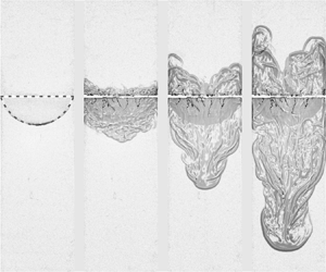
Figures 6(a,b) illustrate the evolution of the 3-D single-mode RTI in cases  $A0.40\#1$ and $A0.50\#1$, respectively. Background subtraction maintains the outline of the initial soap film in all images. Following the rupture of the soap film, a single coherent spike penetrates downwards at the centre, while balanced bubbles form at the four corners, completing reflective symmetry ( $\tau =1.0$). This process involves the presence of small vortices. The small vortices within the top box merge into two sizeable bubbles, positioned near the left and right edges of the visualization window ( $\tau =2.0\unicode{x2013}3.0$). Concurrently, the vortices within the bottom box merge into a single, prominent spike located at the centre. As time progresses, the two bubbles continue their ascent, while the head of the spike becomes a mushroom-like shape ( $\tau =4.0\unicode{x2013}5.0$). Additionally, we observed that the boundary layer on the walls causes the heads of bubbles to slightly deviate from the side walls. Details on the boundary layer can be found in Appendix B.

Figure 6. Shadow images of the evolution of RTI in (a) the  $A0.40\#1$ case and (b) the $A0.50\#1$ case, with $a_{b}$ and $a_{s}$ denoting the amplitudes of bubbles and spikes, respectively.
3.2. Quantitative analysis
Time-varying dimensionless amplitudes, denoted as  $\eta$ ( $=k_W(a-a_{0})$), in various cases, are measured from experiments and presented in figure 7. The amplitude ( $a$) is defined as the average of the bubble amplitude ( $a_{b}$) and spike amplitude ( $a_{s}$), both labelled in figure 6. Because the error bars for the measured amplitudes are smaller than the symbols themselves, we have chosen not to display the error bars. In the experiment, the soap film undergoes vertical deformation by a significant fraction of its width. As a result, the initial interface is steep and highly curved, potentially leading to immediate growth at a rate inconsistent with the early-time linear regime. The prediction from the linear theory ((1.1), considering $k_W$ as the wavenumber) is indicated by a black line. It has been observed that the linear theory overestimates the experimental data beyond a dimensionless time $\tau =0.2$. Consequently, the subsequent flow quickly transitions to a multi-modal structure after the soap film is punctured, underscoring strong nonlinearity in the early evolution of RTI in this study. Since the deformation of the initial soap film interface is directly influenced by the Atwood number, the departure rate from the linear regime increases with higher Atwood numbers.

Figure 7. Time-varying dimensionless amplitudes measured from experiments. Black and cyan lines represent the predictions of the linear theory and the Guo & Zhang (Reference Guo and Zhang2020) model at  $A=0.50$, respectively.
The dimensionless amplitudes of bubbles  $\eta _{b}$ ( $=k_W(a_{b}-a_{0})$) and spikes $\eta _{s}$ ( $=k_W(a_{s}-a_{0})$) deviate from each other as nonlinear effects become dominant, as shown in figure 8. Because heavier fluids exert a greater drag force on bubbles, while lighter fluids impose a smaller drag force on spikes, the bubble growth is slower than the spike growth. The time-varying amplitude growth rates of bubbles ( $\dot {a}_{b}$) and spikes ( $\dot {a}_{s}$) are respectively calculated by taking the first derivative of time with respect to $a_{b}$ and $a_{s}$, as shown in figure 9. It is found that $\dot {a}_{b}$ saturates around the initial value. In contrast, $\dot {a}_{s}$ increases as time progresses, and then saturates after a dimensionless time $\tau =4.5$. This indicates that the development of bubbles enters the quasi-steady regime from the very beginning, while the development of spikes depends on time and enters the quasi-steady regime at a later time in our experiments.

Figure 8. Time-varying dimensionless bubble amplitudes and spike amplitudes measured from experiments. Pink and cyan lines represent the predictions of the Guo & Zhang (Reference Guo and Zhang2020) model for bubbles using the wavenumber  $k_W$, and spikes using the wavenumber $k_{2W}$, at $A=0.50$, respectively.

Figure 9. The time-varying amplitude growth rates of bubbles and spikes. Symbols represent experimental results in various cases. Pink and cyan lines represent the predictions of the Guo & Zhang (Reference Guo and Zhang2020) model for bubbles using the wavenumber  $k_W$, and spikes using the wavenumber $k_{2W}$, at $A=0.50$, respectively.
The amplitude at which a mode transitions from exponential growth to nonlinear evolution, as anticipated by various late-time models, can be deduced by identifying the time when the linear and nonlinear modal velocities become equal (Ramaprabhu & Dimonte Reference Ramaprabhu and Dimonte2005). This method is commonly employed to model the influence of initial conditions on late-time dynamics (Layzer Reference Layzer1955; Dimonte Reference Dimonte2004). The dimensionless transition bubble amplitude, denoted as  $ka_{b}^{nl}$, can then be calculated using the equation
 \begin{equation} ka_{b}^{nl}=\frac{U_{b}}{\sqrt{Agk_W}}, \end{equation}
where  $U_{b}$ represents the late-time bubble velocity. The expressions for the terminal velocities of bubbles ( $U_{b}$) and spikes ( $U_{s}$) in the quasi-steady regime, derived from various theoretical investigations, are detailed in table 2. Figure 10 illustrates the saturation bubble amplitude $ka_{b}^{nl}$ as a function of the Atwood number $A$, comparing various theoretical models, numerical simulations, and experimental data (the bubble amplitude when the linear growth rate matches the measured growth rate). Our findings demonstrate that the $ka_{b}^{nl}$ values obtained from experiments are consistent with multiple potential flow models (Goncharov Reference Goncharov2002; Guo & Zhang Reference Guo and Zhang2020; Liu et al. Reference Liu, Zhang and Xiao2023), as well as with simulation results (Ramaprabhu & Dimonte Reference Ramaprabhu and Dimonte2005). In cases with lower Atwood numbers, a longer linear regime is observed, possibly attributed to the interface maintaining an approximately sinusoidal shape even at higher amplitudes. Conversely, higher Atwood number cases tend to exhibit square wave characteristics earlier, resulting in the generation of higher-order harmonics on the interface and deviating from the linear regime.
Table 2. The expressions for the terminal bubble velocities ( $U_{b}$) and spike velocities ( $U_{s}$) in the quasi-steady regime, and the corresponding Froude numbers for bubbles ( $Fr_{b}$) and spikes ( $Fr_{s}$).


Figure 10. Nonlinear saturation bubble amplitudes  $ka_{b}^{nl}$ from theoretical models, simulations and experiments as a function of Atwood number $A$. Round symbols represent the numerical results extracted from Ramaprabhu & Dimonte (Reference Ramaprabhu and Dimonte2005), and square symbols represent the present experimental results.
Expressions for bubble Froude numbers ( $Fr_{b}$) and spike Froude numbers ( $Fr_{s}$), from various theoretical studies, are provided in table 2. According to Ramaprabhu et al. (Reference Ramaprabhu, Dimonte, Young, Calder and Fryxell2006) and Wilkinson & Jacobs (Reference Wilkinson and Jacobs2007), $Fr_{b}$ and $Fr_{s}$ can be calculated as
 \begin{equation} Fr_{{b/s}}=\frac{\dot{a}_{{b/s}}}{\sqrt{Ag\lambda/(1\pm A)}}. \end{equation}
Figures 11(a,b) respectively depict the plots of  $Fr_{b}$ and $Fr_{s}$ as functions of their respective values of $\xi _b$ ( $=(a_{b}-a_{0})/\lambda$) and $\xi _s$ ( $=(a_{s}-a_{0})/\lambda$) for all experiments, considering the box width $W$ as the perturbation wavelength $\lambda$, as shown with hollow symbols. The average values of $Fr_{b}$ and $Fr_{s}$ in various cases are presented with solid symbols. These plots also include horizontal lines representing the predictions of the various models listed in table 2.

Figure 11. The variations of (a) the Froude numbers of bubbles  $Fr_{b}$ versus $\xi _b$, and (b) the Froude numbers of spikes $Fr_{s}$ versus $\xi _s$, using the wavenumber $k_W$. Hollow symbols indicate experimental results in various cases, solid symbols indicate their average, and lines indicate the predictions of various models, and similarly hereinafter.
As illustrated in figure 11(a), the experimental values of  $Fr_{b}$ exhibit oscillations around 0.60. The models proposed by Abarzhi et al. (Reference Abarzhi, Nishihara and Glimm2003) for $A\approx 1$ and $A\approx 0$ overestimate the experiments, while the model suggested by Sohn (Reference Sohn2003) for $A=0.50$ underestimates them. In contrast, the average values of $Fr_{b}$ closely resemble the predictions of potential flow models proposed by Goncharov (Reference Goncharov2002) ( $Fr_{b}\approx 0.56$), as well as those by Guo & Zhang (Reference Guo and Zhang2020) and Liu et al. (Reference Liu, Zhang and Xiao2023) for $A=0.50$. This indicates that the late-time behaviour of bubbles is influenced mainly by the spatial constraint imposed by walls. The presence of corners in the channel may contribute to the observed oscillations in $Fr_{b}$ during experiments.
In figure 11(b), the experimental values of  $Fr_{s}$ show a continuous increase over the experimental duration. This suggests that the quasi-steady regime differs between bubbles and spikes, highlighting the asymmetry between them. Consequently, the predictions of the three potential flow models (Goncharov Reference Goncharov2002; Guo & Zhang Reference Guo and Zhang2020; Liu et al. Reference Liu, Zhang and Xiao2023) indicating that $Fr_{s}$ saturates around 0.60 underestimate the experimental observations.
The RTI experiment is conducted with a large initial amplitude, and progresses with a broad spectral signature that is dominated by a fundamental mode. The initial soap film interface in the channel is not purely symmetric, being between a single-mode case and a free-space multi-mode case. The curvature of the spike tip correlates with the entire sinusoidal perturbation, having wavelength  $2W$, as shown in figure 3(a). Thus characterizing the spike instability with a new wavenumber $k_{2W}$ ( $={\rm \pi} /W$) is more appropriate than using $k_W$ ( $=2{\rm \pi} /W$), which considers only the space constrained by walls. We derive a new Froude number ( $Fr_{s}^{new}$) for spikes using $2W$ as the perturbation wavelength, given by the expression
 \begin{equation} Fr_{s}^{new}=\frac{\dot{a}_{s}}{\sqrt{2AgW/(1-A)}}. \end{equation}
Figure 12 presents  $Fr_{s}^{new}$ plots as functions of their respective values of $\xi _{s}^{new}$ ( $=(a_{s}-a_{0})/2W$). We observe that although the experimental values of $Fr_{s}^{new}$ continue to rise, they align with the predictions of potential flow models proposed by Goncharov (Reference Goncharov2002), Guo & Zhang (Reference Guo and Zhang2020) and Liu et al. (Reference Liu, Zhang and Xiao2023) at a later time (corresponding to $\xi _{s}^{new}=0.7$ in figure 12, and $\tau =4.5$ in figure 9). This demonstrates that the late-time evolution of spikes is influenced primarily by the curvature of the initial spike tip.

Figure 12. The variation of the new Froude numbers of spikes  $Fr_{s}^{new}$ versus $\xi _{s}^{new}$, using wavenumber $k_{2W}$ ( $={\rm \pi} /W$).
Then we compare the experiments with the potential flow model developed by Guo & Zhang (Reference Guo and Zhang2020) for 3-D RTI with arbitrary  $A$ using the equations
 \begin{equation} \ddot{a}_{b/s}=-\epsilon_{b/s}k(\dot{a}^2_{b/s}-U_{b/s}^2), \end{equation}
where  $\ddot {a}_{b/s}$ is the second derivative of time with respect to $a_b$ or $a_s$, $k=k_W$ for the bubble and $k=k_{2W}$ for the spike, and $\epsilon _{b/s}$ is expressed as
 \begin{equation} \epsilon_{b/s}=\frac{(1\pm A)(3\pm A)[4(3\pm A)+(9\pm A)\sqrt{2(1\pm A)}]}{2[3+A+\sqrt{2(1\pm A)}][4(3\pm A)+2\sqrt{2(1\pm A)}(4\mp2A)]}. \end{equation}
The Guo & Zhang (Reference Guo and Zhang2020) model's prediction for the average amplitude is depicted by a cyan line in figure 7. Similarly, in figure 8 (or figure 9), the Guo & Zhang (Reference Guo and Zhang2020) model's predictions for bubble amplitudes (or bubble amplitude growth rates) and spike amplitudes (or spike amplitude growth rates) are represented by pink and cyan lines, respectively. These findings suggest that the Guo & Zhang (Reference Guo and Zhang2020) model provides a reasonable description of the 3-D RTI studied here, particularly when taking into account that bubble evolution is affected mainly by spatial constraints from walls, while spike evolution is influenced primarily by the curvature of the initial spike tip.
Since turbulence is required for self-similarity, we calculated the maximum Reynolds number ( $Re$) of the experiments as 4300 using $Re=a\dot {a}/\nu$, with $\nu$ denoting the weighted viscosity coefficient. The maximum $Re$ is larger than the critical value 3700 proposed by Dalziel et al. (Reference Dalziel, Linden and Youngs1999). Therefore, it is reasonable to discuss the self-similar factors for bubbles ( $\alpha _{b}$) and spikes ( $\alpha _{s}$) based on our experiments. As mentioned by Banerjee et al. (Reference Banerjee, Kraft and Andrews2010), one approach to determine the self-similar factors $\alpha _{b}$ and $\alpha _{s}$ is to plot $\sqrt {a_{b}}$ and $\sqrt {a_{s}}$ against $t\,\sqrt {Ag}$, as shown in figure 13. Subsequently, a straight line can be fitted (using the method of least squares) through the linear portion of the curve at a later time (e.g. after dimensionless time 0.4 in figure 13). Squaring the slope of this line yields an averaged value for $\alpha _{b}$ and $\alpha _{s}$. The values of $\alpha _{b}$ and $\alpha _{s}$ in various Atwood number cases, along with their averages, are listed in table 3.

Figure 13. Measurements of self-similar factors for (a) bubbles  $\alpha _{b}$ and (b) spikes $\alpha _{s}$, determined by a linear fitting to $\sqrt {a_{b}}$ and $\sqrt {a_{s}}$ versus $t\,\sqrt {Ag}$.
Table 3. The values of the self-similar factors for bubbles ( $\alpha _{b}$) and spikes ( $\alpha _{s}$) in various cases, and their averages.

Our results indicate  $\alpha _{b}=0.057\pm 0.015$ and $\alpha _{s}=0.173\pm 0.015$. In the similar $A$ studies, Youngs & Read (Reference Youngs and Read1983) found $\alpha _{b}=0.066$ and $\alpha _{s}=0.086$, Kucherenko et al. (Reference Kucherenko, Shibarshov, Chitaikin, Balabin and Pylaev1991) obtained $\alpha _{b}=0.055$ and $\alpha _{s}=0.070$, and Dimonte & Schneider (Reference Dimonte and Schneider2000) acquired $\alpha _{b}=0.050$ and $\alpha _{s}=0.063$. More recently, Roberts & Jacobs (Reference Roberts and Jacobs2016) discovered even smaller values, such as $\alpha _{b}=0.044\pm 0.009$ and $\alpha _{s}=0.057\pm 0.014$ for the immiscible forced experiments. Therefore, the $\alpha _{b}$ value obtained from our experiments is similar to the earlier studies, but the $\alpha _{s}$ value is noticeably higher. It is worth noting that we start with a much larger initial amplitude in the soap film interface ( $a_0/\lambda$ ranges from 0.10 to 0.20, as listed in table 1) compared to previous studies, resulting in strong turbulent mixing zone, which spreads into the spike (Sharp Reference Sharp1984). Additionally, in the current experiment, the spike spans only one wavelength, contrasting with previous unconstrained RTI studies. Because of these two possible factors, the spike develops more rapidly compared to previous experiments.
4. Conclusions
We conducted precise experiments on the three-dimensional (3-D) Rayleigh–Taylor instability (RTI) of an SF $_6$–air interface driven by Earth's gravity at an Atwood number ( $A$) ranging from 0.40 to 0.50. To eliminate small-scale disturbances and diffusion layers, we employed a soap film technique to create a discontinuous gaseous interface. The relationship between the initial interface perturbation and the Atwood number was determined. Spectrum analysis revealed that the initial perturbation of the soap film interface is half the size of an entire single-mode one.
The radial propagation of soap films bursting from the point of piercing creates a broadband perturbation in the surrounding gas on both sides. Since the initial soap film interface is steep and highly curved, the early-time evolution of RTI exhibits strong nonlinearity. The experimental transition of a mode from exponential growth to nonlinear evolution in bubble amplitude aligns well with various potential flow models (Goncharov Reference Goncharov2002; Guo & Zhang Reference Guo and Zhang2020; Liu et al. Reference Liu, Zhang and Xiao2023) and previous simulations (Ramaprabhu & Dimonte Reference Ramaprabhu and Dimonte2005). Later, bubbles grow at a slower rate than spikes as nonlinear effects become dominant.
In the quasi-steady regime, we accurately predicted the bubble Froude number using various potential flow models (Goncharov Reference Goncharov2002; Guo & Zhang Reference Guo and Zhang2020; Liu et al. Reference Liu, Zhang and Xiao2023) by considering the box width  $W$ as the perturbation wavelength, indicating that the late-time evolution of bubbles is influenced mainly by the spatial constraints imposed by walls. Differently, the spike Froude number can be described effectively by these potential flow models by considering the wavelength of the entire sinusoidal perturbation $2W$, illustrating that the late-time evolution of spikes is affected primarily by the curvature of the initial spike tip. Therefore, the quasi-steady regime for bubbles and spikes is different, highlighting the asymmetry of bubbles and spikes. The recent potential flow model (Guo & Zhang Reference Guo and Zhang2020) was employed appropriately to describe well the time-varying perturbation growth induced by 3-D RTI.
The self-similar factors for bubbles ( $\alpha _{b}$) obtained from our experiments match previous research at similar $A$, but the self-similar factors for spikes ( $\alpha _{s}$) are notably larger than in previous studies. The large amplitude in the initial soap film interface with a 3-D single-mode perturbation may lead to strong turbulent mixing zone, promoting the development of spikes.
Funding
This work was supported by Tamkeen under the NYU Abu Dhabi Research Institute grant CG002.
Declaration of interests
The authors report no conflict of interest.
Appendix A. Background subtraction
Throughout the sequence, we implemented background subtraction on the images, excluding the final image before the soap film is ruptured. This approach preserves the outline of the initial soap film across all images. As an example, figure 14 illustrates the background subtraction process for the image at  $\tau =5$ in the $A0.50\#1$ case. We utilized the ‘Photron FASTCAM Viewer 4’ software to subtract the image at $\tau =0$ from the image at $\tau =5$, applying a greyscale threshold from 0 to 10. This process yielded an improved image showing the interfacial morphology. Additionally, the black streaks observed near the initial interface position in the $\tau =5$ image are shadows caused by the bursting soap film. Some bursting soap films adhered to the acrylic of the tank. Moreover, in the $\tau =0$ image, the dark horizontal region near the initial interface signifies the boundary between the top and bottom boxes. After background subtraction, the boundary in the consecutive image is determined by subtracting the background image's boundary, resulting in a white horizontal area between bubbles and spikes.

Figure 14. Sketch of the background subtraction process for experimental images.
Appendix B. Boundary layer thickness
We evaluated the thickness of the boundary layer on the walls as it may impact bubble evolution. To simplify calculations, we assumed laminar and incompressible flow throughout the experiment. Consequently, the displacement thickness of the boundary layer ( $\delta ^*$) can be approximated using the formula
 \begin{equation} \delta^*=1.72\,\sqrt{\frac{\nu a_b}{\dot{a}_b}}, \end{equation}
where  $a_b$ is the bubble amplitude, $\dot {a}_b$ is the bubble amplitude growth rate, and $\nu$ is the weighted viscosity coefficient. Figure 15 shows the time-varying boundary layer thickness in various cases. We note a linear increase in $\delta ^*$ until a dimensionless time $\tau =2.0$, beyond which the rate of increase in $\delta ^*$ levels off. Finally, $\delta ^*$ attains a value 0.045 times the box width at $\tau =5.0$. The boundary layer causes the leading edge of bubbles to slightly deviate from the side walls, as illustrated in figure 6.

Figure 15. Time-varying displacement thickness of boundary layer on walls.


