2 Mathematical model

2.1 Governing equations

The theoretical simulation is focused on the two-dimensional linear stability analysis of a fluid saturated horizontal porous layer of height $H$ , see figure 1. The horizontal boundary planes are assumed to be impermeable and isothermal at temperature $T_{0}+\unicode[STIX]{x0394}T$ , lower boundary, and $T_{0}$ , upper boundary. Darcy’s law generalised for non-Newtonian power-law fluids is here employed together with the Oberbeck–Boussinesq approximation. Local thermal equilibrium between the solid and the fluid phase is assumed and a convection–diffusion energy balance is used to model the heat transfer. The balance equations and the boundary conditions can be written in the dimensionless form

(2.1) $$\begin{eqnarray}\left.\begin{array}{@{}c@{}}\unicode[STIX]{x1D735}\boldsymbol{\cdot }\boldsymbol{u}=0,\\ \unicode[STIX]{x1D735}\times [\unicode[STIX]{x1D702}(T)|\boldsymbol{u}|^{n-1}\boldsymbol{u}]=Ra\unicode[STIX]{x1D735}\times (T\boldsymbol{e}_{y}),\\ \displaystyle \frac{\unicode[STIX]{x2202}T}{\unicode[STIX]{x2202}t}+\boldsymbol{u}\boldsymbol{\cdot }\unicode[STIX]{x1D735}T=\unicode[STIX]{x1D6FB}^{2}T,\\ y=0:\quad v=0,T=1,\quad \text{and}\quad y=1:\quad v=0,T=0\end{array}\right\}\end{eqnarray}$$

by introducing the transformations

(2.2a-d ) $$\begin{eqnarray}(x,y)\rightarrow H(x,y),\quad (u,v)\rightarrow {\displaystyle \frac{\unicode[STIX]{x1D718}}{H}}(u,v),\quad t\rightarrow {\displaystyle \frac{\unicode[STIX]{x1D70E}H^{2}}{\unicode[STIX]{x1D718}}}t,\quad T\rightarrow (T_{0}+\unicode[STIX]{x0394}T)T.\end{eqnarray}$$

The Rayleigh number $Ra$ is defined as

(2.3) $$\begin{eqnarray}Ra=\frac{\unicode[STIX]{x1D70C}_{0}g\unicode[STIX]{x1D6FD}\unicode[STIX]{x0394}TKH^{n}}{\unicode[STIX]{x1D707}_{0}^{\ast }\unicode[STIX]{x1D718}^{n}}.\end{eqnarray}$$

Here, $\boldsymbol{u}$ is the seepage velocity having Cartesian components $(u,v)$ , and $(x,y)$ are the Cartesian coordinates, with $y$ denoting the vertical axis, $T$ is the temperature, $\unicode[STIX]{x1D707}^{\ast }$ is the consistency index of the fluid and $\unicode[STIX]{x1D707}_{0}^{\ast }$ (SI unit ( $\text{Pa s}^{n}$ )) denotes the value of $\unicode[STIX]{x1D707}^{\ast }$ evaluated at reference temperature $T_{0}$ , $n$ is the power-law index, $K$ is the permeability (with SI unit $\text{m}^{n+1}$ ), $\unicode[STIX]{x1D70C}_{0}$ is the fluid density at the reference temperature $T_{0}$ , $\boldsymbol{g}$ is the gravitational acceleration (of modulus $g$ ), $\unicode[STIX]{x1D6FD}$ is the thermal expansion coefficient of the fluid, $\unicode[STIX]{x1D70E}$ is the ratio between the average volumetric heat capacity of the porous medium and the volumetric heat capacity of the fluid, and $\unicode[STIX]{x1D718}$ is the average thermal diffusivity of the saturated porous medium. We assume here the following dependence of $\unicode[STIX]{x1D702}$ on $T$ (Nowak, Gryglaszewski & Stacharska-Targosz Reference Nowak, Gryglaszewski and Stacharska-Targosz1982; Celli et al. Reference Celli, Barletta, Longo, Chiapponi, Ciriello, Di Federico and Valiani2017):

(2.4) $$\begin{eqnarray}\unicode[STIX]{x1D702}(T)={\displaystyle \frac{\unicode[STIX]{x1D707}^{\ast }(T)}{\unicode[STIX]{x1D707}_{0}^{\ast }}}=(1+\unicode[STIX]{x1D6FE}\,Ra\,T)^{-n},\end{eqnarray}$$

where $\unicode[STIX]{x1D6FE}$ is a non-negative dimensionless parameter that tunes the departure from the constant consistency index model, namely

(2.5) $$\begin{eqnarray}\unicode[STIX]{x1D6FE}=\frac{\unicode[STIX]{x1D707}_{0}^{\ast }\,\unicode[STIX]{x1D718}^{n}\,\unicode[STIX]{x1D709}}{\unicode[STIX]{x1D70C}_{0}\,g\,\unicode[STIX]{x1D6FD}\,K\,H^{n}},\end{eqnarray}$$

where $\unicode[STIX]{x1D709}$ is a fluid property (with unit $\text{K}^{-1}$ ) modulating the slope of the temperature change. In passing, we note that an exponential dependence is modelled in Darbouli et al. (Reference Darbouli, Métivier, Leclerc, Nouar, Bouteera and Stemmelen2016). A comparison between the two models is reported in the supplementary material, showing that both models can be used, with a similar agreement between experimental data and interpolating function.

2.2 Basic solution and stability analysis

The stability analysis has to be performed on a stationary solution of the balance equations (2.1). This solution is the so-called basic state, here denoted by the subscript  $b$ . The stationary solution of (2.1) here considered as basic state is

(2.6) $$\begin{eqnarray}u_{b}=Pe\left[1+{\displaystyle \frac{\unicode[STIX]{x1D6FE}\,Ra\,(1-2\,y)}{2+\unicode[STIX]{x1D6FE}\,Ra}}\right],\quad v_{b}=0,\quad T_{b}=1-y,\end{eqnarray}$$

where $\boldsymbol{u}_{b}=\{u_{b},v_{b}\}$ is the basic state velocity vector, and the Péclet number is defined as the mean velocity of the basic flow, given by

(2.7) $$\begin{eqnarray}Pe=\int _{0}^{1}u_{b}\,\text{d}y.\end{eqnarray}$$

As the experimental set-up is composed by a Hele-Shaw cell, the basic state in (2.6) and (2.7) is two-dimensional. Accordingly, in the following, a two-dimensional linear stability analysis in the plane $(x,y)$ is performed.

The basic state is thus perturbed by small-amplitude disturbances, namely

(2.8) $$\begin{eqnarray}\boldsymbol{u}=\boldsymbol{u}_{b}+\unicode[STIX]{x1D700}\,\boldsymbol{U},\quad T=T_{b}+\unicode[STIX]{x1D700}\,\unicode[STIX]{x1D6E9},\end{eqnarray}$$

where $\boldsymbol{U}=(U,V)$ is the perturbation velocity, $\unicode[STIX]{x1D6E9}$ is the perturbation temperature, and $\unicode[STIX]{x1D700}$ is a parameter such that $|\unicode[STIX]{x1D700}|\ll 1$ . The streamfunction, $\unicode[STIX]{x1D6F9}(x,y)$ , formulation can be employed to simplify the problem, with $U=\unicode[STIX]{x2202}\unicode[STIX]{x1D6F9}/\unicode[STIX]{x2202}y$ and $V=-\unicode[STIX]{x2202}\unicode[STIX]{x1D6F9}/\unicode[STIX]{x2202}x$ . The perturbations can now be expressed in terms of normal modes, namely

(2.9) $$\begin{eqnarray}\left\{\begin{array}{@{}l@{}}\unicode[STIX]{x1D6F9}(x,y,t)\\ \unicode[STIX]{x1D6E9}(x,y,t)\end{array}\right\}=\left\{\begin{array}{@{}l@{}}f(y)\\ h(y)\end{array}\right\}\exp (\unicode[STIX]{x1D706}\,t)\exp [\text{i}(k\,x-\unicode[STIX]{x1D714}\,t)].\end{eqnarray}$$

One can substitute (2.8) and (2.9) into (2.1) to obtain

(2.10) $$\begin{eqnarray}\left.\begin{array}{@{}c@{}}n(n-1)Gu_{b}^{\prime }\,f^{\prime }+nu_{b}[Gf^{\prime \prime }+G^{\prime }(f^{\prime }-hu_{b}^{\prime })]-k^{2}Gu_{b}\,f\\ -u_{b}^{2}(G^{\prime \prime }h+G^{\prime }h^{\prime })+\text{i}kRau_{b}^{2-n}h=0,\\ h^{\prime \prime }-h(k^{2}+\unicode[STIX]{x1D706}-\text{i}\unicode[STIX]{x1D714}+\text{i}ku_{b})-\text{i}kf=0,\quad \text{with }f=0,h=0\text{ at }y=0,1,\end{array}\right\}\end{eqnarray}$$

where the primes denote derivatives with respect to $y$ and $G(y)=\unicode[STIX]{x1D702}(T_{b}(y))$ . We note that, due to (2.10), we have $\text{d}\unicode[STIX]{x1D702}(T_{b})/\text{d}T_{b}=-G^{\prime }(y)$ .

2.3 Derivation of critical wavenumber and Rayleigh number

The solution of (2.10) is obtained numerically by employing the same procedure used in Celli et al. (Reference Celli, Barletta, Longo, Chiapponi, Ciriello, Di Federico and Valiani2017). The critical values of the Rayleigh number and of the wavenumber are reported in figures 2 and 3 as functions of the parameter $\unicode[STIX]{x1D6FE}$ for different values of the power-law index $n$ and of the Péclet number. As $Pe$ increases, these figures illustrate the non-monotonic behaviour of $Ra_{c}$ and $k_{c}$ versus $\unicode[STIX]{x1D6FE}$ .

Figure 2.

Critical values of the Rayleigh number.

Figure 3.

Critical values of the wavenumber.

Figure 4.

Layout of the Hele-Shaw cell.

3 Experimental set-up

Validation of the model was performed by comparison of the theoretical results achieved in § 2 with experimental results obtained with an analogue model consisting of a Hele-Shaw cell 80 cm long and 4 cm high; its design is similar to Hartline & Lister (Reference Hartline and Lister1977), see figure 4(a,b). A frame of aluminium held together two polycarbonate windows 0.8 cm thick, with a gap variable between 0.1 and 0.3 cm controlled by aluminium shims. The upper and lower frames were cooled and heated, respectively, by a water flux within PVC pipes inserted into the frame. Temperature control within 0.1 K was achieved via two thermostatic baths. The temperature was measured with two probes inserted in the upper and lower side of the frame: PT100 4 wires AA 1/3DIN with a nominal accuracy of 0.1 K at 273 K. The probes were calibrated in a limited range of temperature with a maximum uncertainty of 0.08 K, hence the error on the temperature difference between the two frames is 0.12 K. The cell is insulated with foam rubber in order to avoid lateral dispersion – except for a window in the central section to allow observation of the fluid flow. The uniform horizontal velocity component, representing the basic flow, was obtained by injecting fluid with a syringe pump in one of the two wells, with overflow in the other well. The visualisation of the flow field was obtained with a tracer having the same composition as the fluid within the cell, i.e. water and Xanthan Gum (nominal concentration in the range 0.10 %–0.20 %, the actual one is a little smaller because the mixture was filtered to eliminate some lumps for homogeneity), added with aniline dye. The tracer was injected through several small holes with diameter less than 0.1 mm in a PVC pipe inserted in one of the polycarbonate windows, positioned at mid-height of the window. The pipe was connected to two small tanks, periodically refilled with tracer fluid, in order to guarantee a constant and uniform injection. The images were acquired with a USB video camera ( $1280~\text{pixel}\times 960~\text{pixel}$ ) with microscope lenses, with a field of view (FOV) of ${\approx}12\times 10~\text{cm}^{2}$ . The FOV was illuminated by a lamp with rays made parallel through a lens, in order to increase resolution and sharpness. The video camera acquired a single frame each 30–60 s. The overall process was controlled by a PC with a DAQ board, storing temperature measurements at a data rate of 10 Hz, and controlling the USB image acquisition. Tracer was progressively injected and the temperature set-up was increased/lowered for the hot/cold thermostatic bath, with steps of 0.1 K each 2–3 min. Variations of the upper/lower temperature were fixed in order to have a constant (or almost constant) temperature $T_{0.5}$ in the mid section. Most experiments lasted for 3–4 h, with a time gradient of temperature of less than $10^{-3}~\text{K}~\text{s}^{-1}$ . A typical time series of measured temperatures is shown in the supplementary material, as well as details of rheometric measurements and experimental uncertainties.

Table 1.

Parameters of the experiments. Here, $\unicode[STIX]{x1D70C}_{0}$ is the reference mass density at a temperature of 298 K, $\unicode[STIX]{x1D707}_{0}^{\ast }$ is the fluid consistency index, evaluated at the reference temperature $T_{0}$ , $n$ is the fluid behaviour index, $b$ is the gap width, $\overline{u}_{b}$ is the average basic horizontal velocity, $T_{0.5}$ is the temperature in the mid section $z/H=0.5$ during experiments (minimum/maximum value), $Pe$ is the Péclet number, $Ra_{c,exp}$ is the experimental critical Rayleigh number, $k_{c,exp}$ is the dimensionless critical wavenumber. Expt., experiment.

4 Experimental results

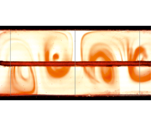
The experiments and their parameters are listed in table 1. Figure 5 shows a typical sequence of frames from the early stages of instability development to the appearance of strongly nonlinear instabilities. A slow translation to the left is observed due to the basic flow velocity of $0.0087~\text{cm}~\text{s}^{-1}$ . Similar results were obtained for all tests. In most cases, the temperature difference between the two frames first showed an increase over time, followed by a reduction, with consequent linearisation of the convective cells up to their disappearance. Hysteresis phenomena, with a difference in temperature at the early appearance of the cell (branch of rising $\unicode[STIX]{x0394}T$ ) higher than the difference in temperature corresponding to the return to stability (branch of reducing $\unicode[STIX]{x0394}T$ ), were evident only for the more viscous fluid flow. The description of the methodology adopted for comparison gives evidence of the numerous experimental complexities encountered during the activity.

Figure 6(a,b) shows the comparison between the theoretical and experimental critical Rayleigh number for two different groups of experiments with different values of the Péclet number $Pe$ . The error bars are shown for the experiments and represent one standard deviation. The theoretical predictions are supplemented with confidence limits corresponding to the possible combinations of the variables and parameters involved in the model, assumed equal to their nominal value plus/minus their standard deviation.

The value of theoretical $Ra_{c}$ increases for increasing fluid behaviour index, although not monotonically for the larger value of $Pe$ considered; also, an increase in $Pe$ brings about an increase in $Ra_{c}$ , albeit not in the same proportion for different values of $n$ . These theoretical values consistently overpredict experimental values to various degrees, from approximately 15 % to nearly 100 %; no clear trend is detected in the discrepancy for different values of $n$ and/or $Pe$ . The experimental values of $Ra_{c}$ obtained show a non-monotonic behaviour with fluid behaviour index $n$ ; for both $Pe$ values, a minimum for $Ra_{c}$ is evident at $n=0.6$ .

Figure 5.

Evolution of the perturbation over time (top to bottom and left to right) for one of the experiments. The vertical lines delimit squares with side length equal to $H=4~\text{cm}$ . In the final frame (bottom right) a bifurcation of the cell in a strongly nonlinear regime is observed. Snapshots are 60 s apart.

Figure 6.

Comparison of the experimental and theoretical values of the critical Rayleigh number (a) for $Pe=34\pm 2$ and (b) for $Pe=52\pm 2$ , and of the critical wavenumber (c) for $Pe=34\pm 2$ and (d) for $Pe=52\pm 2$ . Open symbols are the experiments, curves are theory. The error bars and the confidence bands refer to one standard deviation. Here, $k_{cN}=\unicode[STIX]{x03C0}$ is the critical wavenumber for a Newtonian fluid initially at rest.

Figure 6(c,d) compares the experimental and theoretical values of the critical wavenumber for varying $n$ , again for two different values of $Pe$ . The trend is correctly reproduced and the theoretical formulation always underpredicts the experimental result to a variable degree (the maximum discrepancy is below 10 %), with a lower average discrepancy for experiments at low Péclet number.

There are several sources of discrepancy: the strong nonlinearity of the flow field favours a rapid evolution of the cell from the onset of instability towards a fully developed cell with a reduction of wavelength (and consequent increment of the experimental wavenumber). A further evolution leads to doubling of the cells. A disturbing factor is a possible slip at the wall, which is not included in the model and which reduces the flow resistance and favours the growth of the instability. This effect was clearly detected for viscoplastic fluids (Darbouli et al. Reference Darbouli, Métivier, Piau, Magnin and Abdelali2013), and is widely documented for most aqueous polymer solutions – see Joshi, Lele & Mashelkar (Reference Joshi, Lele and Mashelkar2000) and Valdez et al. (Reference Valdez, Yeomans, Montes, Acuña and Ayala1995).

5 Discussion and conclusions

The need to extend the available models for Darcy–Bénard instability to rheologically complex fluids and non-viscometric flow fields has suggested the analysis of non-Newtonian fluid flow in a two-dimensional geometry and in the presence of a uniform cross-flow. The fluid is assumed to display a power-law nature with temperature-dependent consistency index. A two-dimensional linear stability analysis in the vertical plane yields the critical wavenumber and the critical Rayleigh number upon solving numerically the eigenvalue problem. The critical Rayleigh and wavenumbers are significantly affected by the power-law index and by the thermal effects on the consistency index, displaying a non-monotonic trend with local minima and maxima.

A set of experiments performed in a Hele-Shaw cell allowed us to study flow patterns as functions of the Rayleigh number. The experiments were carried out with shear-thinning fluids of flow behaviour index $n$ ranging from 0.55 to 0.72, coupled with cell gap widths of 0.2 or 0.3 cm, imposing cross-flow velocities of approximately $0.01~\text{cm}~\text{s}^{-1}$ and vertical temperature gradients of $0.5{-}3.4~\text{K}~\text{cm}^{-1}$ between the lower and upper frames. The critical wavenumber was obtained via analysis of the frames acquired.

The overall flow dynamics is controlled by the entangled interaction between fluid properties, geometry of the flow field and underlying uniform cross-flow. The onset of convective cells occurs with increasing wavenumber for increasing $n$ . At the onset of convection, the shear-thinning behaviour favours a fast growth of the instabilities. Considering the complexity of the protocol and the numerous sources of uncertainty (see Longo et al. (Reference Longo, Di Federico, Chiapponi and Archetti2013b ), for details on uncertainties in rheometric measurements), experimental results show a fairly good agreement, within 10 %, with theory for the critical wavenumber. The discrepancy may be attributed to nonlinear phenomena not captured by the linear stability analysis, and additionally to slip at the wall, and ageing and degradation of the fluid properties – all unaccounted-for phenomena in the theoretical model.

Results for the critical Rayleigh number show a correct trend and an overall acceptable agreement with theoretical predictions; the discrepancy varies widely with $n$ and $Pe$ values, and is generally larger than for the critical wavenumber. The theoretical model itself shows a larger sensitivity to the governing parameters for $Ra_{c}$ than for $k_{c}$ . Other rheological models, more complex than the power law, are available to describe Xanthan Gum mixtures (see, for example, Escudier et al. (Reference Escudier, Gouldson, Pereira, Pinho and Poole2001), where a Carreau–Yasuda model is favourably tested). However, the power-law model is suitable to locally describe complex rheologies, with several validations in complex flows geometries – see Longo et al. (Reference Longo, Di Federico, Archetti, Chiapponi, Ciriello and Ungarish2013a ) and the recent Chiapponi et al. (Reference Chiapponi, Ciriello, Longo and Di Federico2019). In this regard, we have verified that in the shear rate range of our experiments, a power-law model adequately fits the rheometric data – see figure 1(b) and its caption in the supplementary material.

The experiments showed clearly that the development of the instability may occur at a threshold Rayleigh number lower than the critical value predicted by linear stability theory. This could be considered as symptomatic of a subcritical bifurcation, induced by the nonlinear terms in the governing equations of the fluid. Indeed, it is well established, both experimentally and theoretically, that the bifurcation is supercritical in the Darcy–Bénard convection with throughflow for a Newtonian fluid. The supercritical linear threshold of absolute instability (see Barletta Reference Barletta2019) was found to correspond perfectly to the one needed in experiments to trigger the instability. As suggested by the present series of experiments, as well as by the shear-thinning behaviour (see Balmforth & Rust Reference Balmforth and Rust2009; Albaalbaki & Khayat Reference Albaalbaki and Khayat2011; Bouteraa et al. Reference Bouteraa, Nouar, Plaut, Métivier and Kalck2015), the nature of the bifurcation may be subcritical, and therefore a nonlinear stability analysis has to be carried out as a natural development of the present study. By using the concepts of nonlinearly convective and absolute instability, as defined in Couairon & Chomaz (Reference Couairon and Chomaz1997), one can hope to obtain results that corroborate the experimental results obtained in this paper.

The present study can be extended in several directions. In particular, a change of the boundary condition (open instead of closed top) in the experimental set-up could give further hints for understanding the complex evolution of the cells; a direct numerical simulation should be at hand, due to the viscous regime of the flow field. The great flexibility of numerical experiments could shed light on the possible effects of slip at the wall and on the evolution in the quasi-linear and fully nonlinear regimes. Additional topics to be investigated are related to vertical fractures with uneven gaps (for example, see Felisa et al. (Reference Felisa, Lenci, Lauriola, Longo and Di Federico2018)), which are good proxies of geological fractures characterised by a length scale from a few centimetres to several metres and subject to thermal gradients and cross-flow. The vertical convection should be a quite efficient agent for re-mixing the fluid, favouring heat exchange and chemical reactions.