


1. INTRODUCTION
Wind-packing is the process of snow hardening under the influence of wind. Snow covers in alpine and polar regions often contain the resulting wind slabs or wind crusts. Such layers are relevant for the avalanche danger in alpine areas and they affect the interaction between the snow cover and the atmosphere. In polar regions, wind-packing influences the mass balance, as new snow is often only immobilized through hardening (Groot Zwaaftink and others, Reference Groot Zwaaftink2013).
Many studies describe wind-packed snow qualitatively (e.g. Schytt, Reference Schytt1958; Benson, Reference Benson1967; Alley, Reference Alley1988). However, it remains unclear how these layers form. Many processes have been proposed but real evidence is scarce. Some authors focus on humidity and see wind-packing as ‘firnification accelerated by a wet wind’ (Seligman, Reference Seligman1936). According to Benson (Reference Benson1967), Schytt (Reference Schytt1958) and Seligman (Reference Seligman1936) the wind leads to an increased vapour flux, which causes rapid sintering of the snow. The only condition is that the air humidity must be above 85% because a dry wind would sublimate some of the snow and therefore loosen it (Seligman, Reference Seligman1936). There is debate about whether the extra humidity is deposited directly from the humid air or whether some of the snow is sublimated and redeposited within the snowpack. Several authors see the mechanical fragmentation of snow crystals by the wind and their subsequent sintering as the main process behind wind-packing (Kotlyakov, Reference Kotlyakov1966; Endo and Fujiwara, Reference Endo and Fujiwara1973; Alley, Reference Alley1988; Colbeck, Reference Colbeck1991; Guyomarc'h and Mérindol, Reference Guyomarc'h and Mérindol1998; Kozak and others, Reference Kozak, Elder, Birkeland and Chapman2003; Fierz and others, Reference Fierz2009). This process can only happen in a saltation layer, where snow particles collide with each other and with the surface. This is in contrast to the ‘accelerated firnification’, which could also happen without drifting snow.
This paper aims at answering the question whether saltation is a prerequisite for wind-packing or not by observing the formation of wind crusts in a wind tunnel. The gained insight could be useful to improve the implementation of wind-packing in snow-cover models. This would in turn improve stability assessments and avalanche danger forecasts.
2. METHODS
2.1. Wind tunnel
A straight, open-circuit, boundary-layer wind tunnel has been in operation at SLF since 2001 (e.g. Clifton and others, Reference Clifton, Rüedi and Lehning2006; Walter and others, Reference Walter, Horender, Voegeli and Lehning2014; Crivelli and others, Reference Crivelli, Paterna, Horender and Lehning2016; Paterna and others, Reference Paterna, Crivelli and Lehning2016). However, this facility is not suited to investigate wind-packing. In an open-circuit wind tunnel, any drifting particles are ejected within seconds. There is not enough time for mechanical fragmentation and subsequent sintering. We need a closed-circuit configuration or ideally an infinite fetch. An annular or obround wind tunnel is a way to achieve that. There already are some closed-circuit wind tunnels adapted for cryospheric studies, such as the Cryospheric Environment Simulator (CES) in Shinjo, Japan (Sato and others, Reference Sato, Kosugi and Sato2001) or the Jules Verne wind tunnel at the Centre Scientifique et Technique du Bâtiment (CSTB) in Nantes, France (Naaim-Bouvet and others, Reference Naaim-Bouvet, Naaim and Michaux2002). But these facilities use snow tables of a limited size and can therefore not mimic an infinite fetch. Annular wind tunnels of various sizes have been built at the University of Heidelberg to investigate air-sea gas transfer under different water surface conditions (e.g. Münnich and others, Reference Münnich, Favre and Hasselmann1978; Jähne, Reference Jähne1980; Schmundt and others, Reference Schmundt, Münsterer, Lauer, Jähne, Jähne and Monahan1995; Krall, Reference Krall2013). The idea of simulating an infinite fetch with such a shape is therefore not new.
Our new wind tunnel has an obround shape as can be seen in Figure 1. The two straight sections provide additional space for measurements as compared with an annular design and are not subject to centrifugal effects like the curved parts. The wind tunnel has an overall length of 2.2 m and a width of 1.2 m. The channel is 20 cm wide and 50 cm high. The airflow is created by a model-aircraft propeller driven by an electric motor. Free stream wind speed of up to 8 m s−1 can be reached. A vibrating sieve can be used to simulate snowfall. This is useful to obtain drifting snow at wind speeds below the actual saltation threshold.

Fig. 1. The wind tunnel on its 1.5 m wide and 2.5 m long platform. It is located in the same building as the straight wind tunnel. The arrow indicates the direction of the airflow. The cover openings allow a basic control over the temperature and humidity in the wind tunnel. Insert (a) shows the main test section with the camera above the windows and the sensors to the left. Insert (b) shows the sensors listed in Table 1 at the upstream end of the main test section. 1: MiniAir, 2: Rotronic, 3: SI-131, 4: Pt100. The snow surface is usually between the Pt100 and the bottom Rotronic sensor. The Pt100 is inserted after lowering the tunnel onto the snow.
Before each experiment, 10–30 cm of fresh snow are collected on a pair of wooden trays outside the building (Fig. 2a). The wind tunnel, which is open at the bottom, is lifted by crane and the trays are arranged underneath it (Fig. 2b). Finally, the wind tunnel is lowered into the snow cover (Fig. 2c). As a result, we have a continuous cover of almost undisturbed, natural snow in the wind tunnel. Each experiment consisted usually of several wind periods. Different measurements were performed before and after each one. Wind periods were often 30 min or 1 h long but could be as short as a few minutes or as long as several hours.

Fig. 2. Operation of the wind tunnel. (a) Snow is collected on trays and (b) arranged below the wind tunnel. (c) Then, the wind tunnel is lowered into the snow. (d) The SnowMicroPen (SMP) during a measurement. The SMP is the main instrument.
The flow quality in this wind tunnel cannot be compared with standards of wind tunnels used for aerodynamic testing. The high curvature, the narrow channel, the use of a propeller as a wind source and the unsteady snow surface make for a chaotic flow. It is therefore not possible to make quantitative statements about the interaction of the flow with saltating particles for example. However, we are certain that this facility is adapted to test whether drifting snow is necessary for wind-packing or not. More details about the design and flow characteristics of the wind tunnel can be found in the Appendix.
2.2. Instrumentation
The instrumentation in the wind tunnel is located in the second straight section downstream of the motor, called the main test section (Fig. 1). The measured parameters are wind speed, air humidity, air temperature, snow surface temperature and snow temperature. Air humidity and air temperature are measured at three heights. Table 1 lists the used sensors. The data are acquired at 5 Hz with LabVIEW through National Instruments CompactDAQ hardware. In addition to the automatic measurements, a mm scale was used to manually measure the snow height in the test section. Unfortunately, this measurement was only reliable while the snow surface was flat, which was usually only the case before experiments or during experiments without drifting snow.
Table 1. Installed sensors and measured parameters
A SnowMicroPen (SMP, Fig. 2d) is used to measure the most important properties of a slab/crust, namely its hardness and thickness. The SMP is a high-resolution constant-speed penetrometer (Schneebeli and Johnson, Reference Schneebeli and Johnson1998; Proksch and others, Reference Proksch, Löwe and Schneebeli2015). The SMP measures penetration resistance, which is directly related to hardness. We are mainly interested in the evolution of the hardness at the surface.
For some experiments, an industrial camera looking down vertically at the surface was used. We attempted to use it to detect drifting snow events by correlating sequences of images. This was not completely reliable. Wind periods with drifting snow were subsequently identified by eye. The camera images were used to create time lapse videos of the experiments. These were helpful to see what happened at the snow surface.
2.3. Postprocessing
The goal of the postprocessing of the SMP measurements (SMPs) is to reduce each force profile to a representative number. That way, large numbers of SMPs can be analysed using statistical methods. First, the location of the snow surface in the profile is determined. An automatic algorithm based on a threshold relative to the force signal in the air applied to a smoothed signal works well. Then, a linear trend is fitted to the signal in the air and subtracted from the force profile. The linear trend always had a negative slope on the order of 10−6 N mm−1 and an offset of ~48 mN. These values are related to the signal amplifier in the SMP and are within the expected range.
To find a representative number for an SMP, we attempted to determine the depth down to which the wind had affected each measurement by comparing the current SMP with the initial measurements. Then, a statistic could be calculated for the signal between the snow surface and this affected depth. Finding this depth was obvious in many cases but sometimes the natural variability of the snowpack, snow settling or other reasons prevented a precise determination. Therefore, the representative number is now defined as the 90% quantile of the force signal in the 10 mm below the snow surface. The advantage of using a high quantile as a representative statistic is that thin crusts can still be detected. If the mean or median were considered they would be averaged out by the unaffected, soft snow below the crust. However, the single number looses descriptive power with respect to the crust if the quantile is too high. For example, if the force signal in the complete snowpack is used, only quantiles higher than 99% were able to detect thin crusts. Considering only the snow close to the surface has another advantage. The hardness of the initial snowpack usually increased with increasing penetration depth. As a result, the overall quantiles characterized the snow close to the bottom. A subsequently formed crust at the surface could therefore only be detected if it was harder than the initial snow at the bottom and this was not always the case. The surface quantiles easily detect such changes. The 90% quantile of the force signal in the topmost centimeter of snow is henceforth referred to as ‘SMP hardness’.
3. RESULTS
In the winters 2015/16 and 2016/17 a total of over 1000 SMP measurements were acquired during 38 experiments. The data are publicly available on Envidat (Sommer and others, Reference Sommer, Lehning and Fierz2017). Figure 3 shows the SMP hardness of all initial SMPs. Usually, four measurements were taken before the beginning of each experiment. Figure 3 shows the spread of the initial conditions. The fresh snow was usually only a few hours and at most about a day old. But depending on the temperature and the wind speed during the snowfall, the initial SMP hardness varied by a factor of three. The standard deviation of initial SMP hardnesses of a single experiment is on average four times lower than the standard deviation of all 148 initial SMP hardnesses (1.9 and 7.3 mN). Each snow cover is therefore fairly homogeneous and the variability in Figure 3 is mainly due to the different snow covers in each experiment. The density of the initial snow was usually measured close to the snow surface and close to the bottom with a 3 cm high box density cutter. The initial density varied between 30 and 94 kg m−3 at the top and between 38 and 124 kg m−3 at the bottom. The correlation between the initial surface densities and the mean initial SMP hardnesses is 0.64.
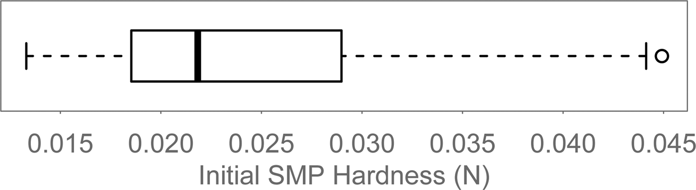
Fig. 3. SMP hardness of 148 initial SMPs showing the variability in the initial conditions.
As a result of the initial variability between the experiments, the following plots will not show absolute SMP hardness but SMP hardness change. The main difficulty with SMP measurements is that only one measurement can be acquired at a specific location. Two measurements must be at least 3 cm apart. At a closer distance, the hole of the first penetration would influence the next measurement. Looking at SMP hardness change is therefore only meaningful if the snow cover was homogeneous at a scale of at least 3 cm before the change happened. As mentioned above, the initial snow cover is quite homogeneous for every experiment. Therefore, changes between the current and the initial conditions can always be calculated. SMP measurements acquired at the same time in different positions showed that wind without saltation has a homogeneous effect on the snow cover. For these experiments, we can therefore assume that the snow cover remains homogeneous and it is possible to look at changes in SMP hardness over single wind periods. The effect of saltation, on the other hand, was strongly heterogeneous. As a result, changes between the current and the initial conditions must generally be used for experiments with drifting snow. A SMP hardness change was calculated by averaging the SMP hardness of the SMPs in the reference group (e.g. the initial SMPs) and subtracting this mean from the SMP hardness of the subsequent measurements.
Figure 4 shows the change in SMP hardness between the initial SMPs and the subsequent measurements grouped by whether there had been saltation or not. For the ‘No Drifting’ SMPs, there had not been any drifting snow in any previous wind period and for the ‘With Drifting’ SMPs there had been drifting snow at least during the last wind period before the measurement. The ‘No Drifting’ group of 114 SMPs has a small variability around a median SMP hardness increase of 2 mN. There are some outliers where the SMP hardness increased by up to 30 mN. The 536 SMPs in the ‘With Drifting’ group have SMP hardness increases up to 1.18 N. The median change, however, is only 95 mN and for many measurements the change was negligible. A SMP hardness of 1 N corresponds about to a hand hardness of ‘1 finger’ (Fierz and others, Reference Fierz2009). A Kruskal–Wallis test confirms that the two groups are different with a p-value of the order 10−16.
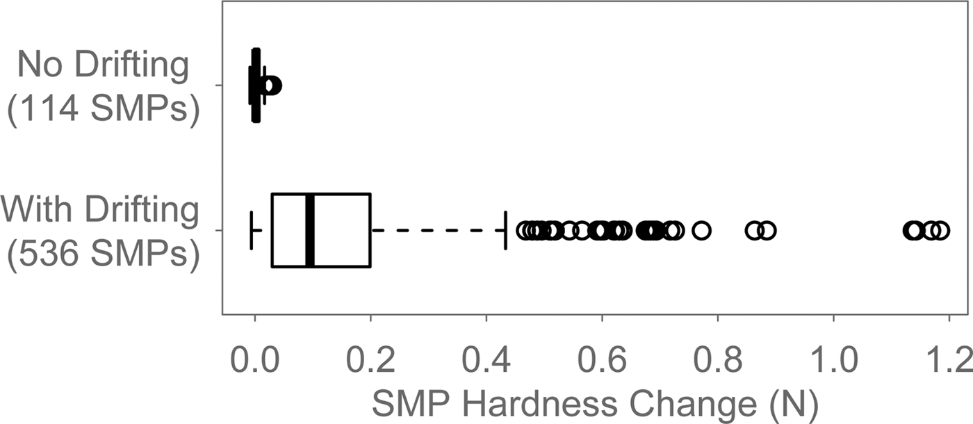
Fig. 4. Comparison of the overall SMP hardness change between SMPs acquired after wind periods with and without drifting snow.
Nine of the ten SMPs with the largest SMP hardness increase in the ‘No Drifting’ group are from an experiment on 6 March 2017. Figure 5 shows averaged SMPs before and after this experiment, which consisted of a single wind period. The hardness increased in the complete snowpack and the snow surface settled by ~4 mm. There was no formation of a crust at the surface. This experiment was quite special because it was very warm. The air temperature was ~1°C during the whole experiment and the snow temperature was ~−1.5°C at the beginning. Furthermore, the wind speed could be increased to 8 m s−1 without initiating saltation. The observed hardening was achieved within 20 min. After that, the experiment was stopped because the snow temperature was reaching 0°C. Similar combinations of decreases of snow depth and overall increases in hardness were also observed in other experiments, where the temperatures and the wind speed were lower but the duration of the wind periods was longer.

Fig. 5. Averaged SMPs before and after an experiment without drifting on 6 March 2017. In 20 min, the snow hardness increased throughout the snowpack and the snow settled considerably. The parentheses in the legend contain the number of SMPs that were used for the average.
According to e.g. Seligman (Reference Seligman1936) a humid wind is able to generate a wind crust without saltation. To reproduce such conditions, an insulated water bowl was placed in the wind tunnel (see Fig. 6) for some of the ‘No Drifting’ experiments. This should saturate the air in the wind tunnel. The water was heated to ~20°C and was usually replaced after it had cooled down to ~5°C, which took ~30 min.

Fig. 6. The water bowl was placed in the snow at the start of the main test section. The bowl was insulated with styrofoam.
Figure 7a compares groups of SMPs taken after wind periods with and without added water. Because only ‘No Drifting’ SMPs are used here, the plot shows the SMP hardness change over single wind periods. The SMP hardness change without added water was, if anything, larger than with added water. The median was 3 mN for the ‘No Water’ group and only 0.3 mN for the ‘With Water’ group. The p-value of the Kruskal–Wallis test comparing the two groups is 0.005. The mean relative humidities during the wind periods in question are shown in Figure 7b. The added water did not have a large effect. The medians are almost equal and the Kruskal–Wallis test shows no significant difference (p-value of 0.29). However, the added water increased the minimum relative humidity from 80 to 90%.
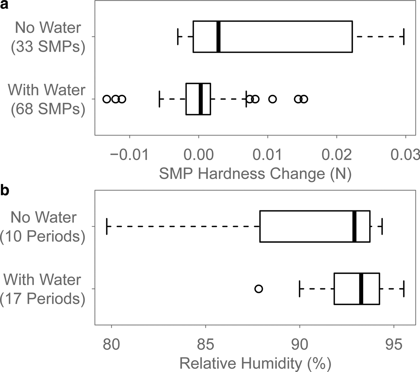
Fig. 7. (a) Comparison of the SMP hardness change in wind periods with and without added water. (b) Comparison of the mean relative humidity during the same wind periods.
During most experiments without drifting snow, additional SMPs were acquired outside the wind tunnel to test whether the wind has any influence at all. The snow in the obround area enclosed by the channel was used for these measurements. Figure 8 shows the comparison between the ‘No Drifting’ SMPs acquired inside the wind tunnel and the corresponding SMPs taken outside the channel. The boxplots show changes over single wind periods. The median is 0.5 mN for the ‘Inside’ SMPs and 0.2 mN for the ‘Outside’ SMPs. The variability is smaller outside than inside. In particular, there are several outliers with higher SMP hardness changes in the ‘Inside’ group (Fig. 5). The p-value of the Kruskal–Wallis test comparing the two groups is 0.1.
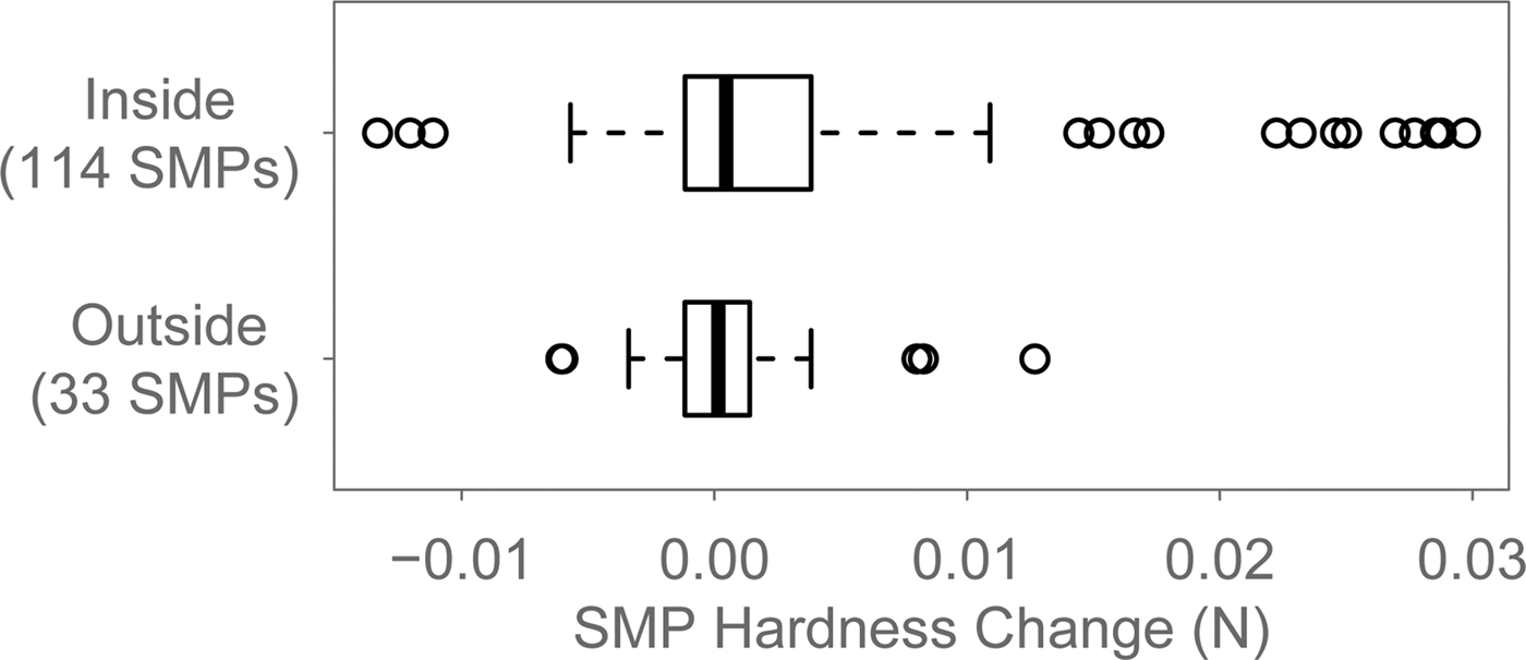
Fig. 8. Comparison of the SMP hardness change in wind periods without drifting and the SMP hardness change measured outside the wind tunnel during the same time periods.
In Figure 4, the striking feature about the ‘With drifting’ boxplot is the large variability of the SMP hardness changes. Figure 9 illustrates this with three SMP measurements from 5 February 2016. SMP1 is one of the initial SMPs. SMP2 was measured after a 15 min wind period at 5 m s−1 with drifting snow and is very similar to SMP1 except that the snow depth decreased by 10 mm. After a second identical wind period, SMP3 was acquired. The snow depth increased by 14 mm and the SMP hardness increased to ~0.3 N. The example shows that similar conditions can have completely different results.

Fig. 9. Three of the SMPs acquired during an experiment on 5 February 2016. SMP1 was acquired at the start of the experiment, SMP2 after the first wind period and SMP3 after the second wind period. Both periods were 15 min long, the wind speed was 5 m s−1 and there was saltation during both periods. The short horizontal lines show the snow surfaces.
4. DISCUSSION AND CONCLUSIONS
The wind tunnel was designed to approximate an infinite fetch with regard to snow saltation. This worked quite well and it was possible to observe the formation of wind crusts. Nevertheless, the experimental setup could certainly be improved. The flow conditions are largely uncontrolled and unknown and this limits the insights that can be gained from this facility. No quantitative statements about the interaction of the flow and the mechanics of wind-packing can be made. Such experiments could perhaps be performed under controlled flow conditions in the facilities at the CSTB or CES mentioned in the introduction. The main constraint for the new wind tunnel was to have an infinite fetch, meaning a continuous and unobstructed cover of natural and undisturbed fresh snow. We do not think that this is possible to achieve in these other facilities. Therefore, while the possibilities of the new wind tunnel may be very limited, we believe it is adapted to gain knowledge about wind-packing in general and to test whether drifting snow is necessary for the formation of wind crusts in particular.
The boxplots in Figure 4 clearly show that no wind crust forms without drifting snow. In some cases, wind without saltation still had a small hardening influence on the snow. An example of this is shown in Figure 5. The hardness increased throughout the snowpack as opposed to only at the surface, the snow depth decreased and the final hardness resulting from this settling and slight compaction was still very low. These processes take place with or without wind but based on the comparison of the ‘Inside’ and ‘Outside’ SMPs in Figure 8 we can assume that wind slightly accelerates them. ‘Wind-accelerated settling and compaction’ sounds very similar to what Seligman (Reference Seligman1936) describes as ‘firnification accelerated by a wet wind’, which is how he defines ‘wind-packing’. This definition is based on experiments where Seligman (Reference Seligman1936) blew either dry or humid air through a column of snow. He noticed that after the passage of dry wind, the snow remained loose while wet wind led to coalescence of the snow. Seligman (Reference Seligman1936) did not really measure the hardness of the resulting snow. Our results show that this process, if at all, hardens snow only slightly and/or slowly. Therefore, we propose to call this process wind-compaction instead of wind-packing.
The added water did not have the expected effect to enhance or accelerate ‘wind-compaction’ or to lead to the actual formation of a wind crust. We also would have expected a larger influence of the added water on the humidity itself. It could be that the sensors become unreliable so close to saturation. It is also likely that the humidity was higher locally, e.g. close to the snow surface. The SMP hardness change with added water was in fact smaller than without added water (Fig. 7a). However, this result is most likely unrelated to the water. The correlation coefficient between the SMP hardness changes and the relative humidities of both groups shown in Figure 7 is −0.37. The fact that the air humidity was always high could be the reason for this absence of correlation. Seligman (Reference Seligman1936) gives a lower limit of 85% air humidity for ‘wind-compaction’ to take place. The humidity in the wind tunnel was almost always above this limit (Fig. 7b). The increased hardening without water as compared to with water is most likely a result of a combination of factors such as temperature, wind speed and wind period duration. We would expect wind-compaction to be more efficient at higher temperatures and higher wind speeds due to the increased heat transfer to the snowpack. There was one experiment without drifting snow and with added water where one measurement showed a SMP hardness increase only at the surface unlike the SMPs in Figure 5. The SMP hardness increased by 20 mN. All other measurements in this experiment, however, showed no hardening. This could mean that the added water can, in some cases, have a local hardening effect on the surface but this measurement could also be attributed to natural variability. Overall, the conclusion remains that no wind crust forms without saltation.
The enormous variability in the ‘With Drifting’ group in Figure 4 needs explaining. Clearly, not all drifting snow events lead to the formation of a wind crust. Saltation is a necessary condition but it is not sufficient. During the experiment shown in Figure 9 some snow was eroded in the main test section during the first wind period. The SMPs acquired afterwards showed no hardening. During the second wind period, in contrast, snow was deposited in the main test section and the subsequent SMPs exhibited a crust at the surface. In this case, the two wind periods in question were short and at the beginning of the experiment. Therefore, it was easy to keep track by eye of where and when snow was eroded and deposited. This was usually not possible. The location of the snow surface in the SMPs can easily be determined but is a bad indicator of erosion or deposition. The wind tunnel, on which the SMP is placed for the measurements, may be oblique relative to the snow surface. In this case, the SMP snow surface location depends on the SMP position in the test section and would lead to wrong estimates of erosion or deposition. Furthermore, there may be a lot of erosion followed by a little deposition in the same wind period. In such cases, the change of the SMP snow surface location only indicates the overall erosion and cannot detect the deposition. The camera in the wind tunnel gives a qualitative idea of when and where snow is either eroded or deposited. The height information, however, is missing and the field of view is very limited. From the few SMP measurements where the erosion or deposition patterns were known, it appears that these processes are vital to understand when a wind crust forms. They could also explain the, sometimes very complicated, shapes of SMP force profiles. To analyse erosion and deposition quantitatively, the wind tunnel will be outfitted with a Microsoft Kinect sensor (Mankoff and Russo, Reference Mankoff and Russo2013). This instrument is a low-cost 3-D scanner and will provide snow depth information at a spatial resolution of less than a centimeter and at a sub-second temporal resolution.
The wind crusts in the wind tunnel reached hardnesses on the order of 1 N. This is significantly harder than the initial snow. However, compared with wind crusts in nature, which can reach a hardness of several Newtons, the snow in the wind tunnel remains relatively soft. This could be due to the relatively low wind speeds in the wind tunnel and the short duration of most experiments.
ACKNOWLEDGEMENTS
We thank Benni Walter, Stefan Horender, Enrico Paterna and Philip Crivelli for their design input and help with experiments. A huge thank you goes to the SLF workshop and electronics lab for working out the detailed design and building the wind tunnel. Research reported in this publication was supported by the Swiss National Science Foundation under grant number 200021_149661.
APPENDIX: DESIGN AND CHARACTERIZATION OF THE WIND TUNNEL
A1. DESIGN OF THE WIND TUNNEL
An infinite-fetch wind tunnel will obviously have a closed-circuit configuration. A typical closed-circuit wind tunnel has a well-defined test section and the circuit is closed with 90° turns with guide vanes, contractions and diffusers. The fan and flow conditioners, such as screens and honeycombs, occupy the complete cross section (Mehta and Bradshaw, Reference Mehta and Bradshaw1979). An infinite fetch cannot be achieved with such a setup. Snow saltation should be able to continue over the snow surface to approximate ‘infinite fetch’ in this particular aspect. Therefore, the complete channel floor (and not just a test section) should be snow-covered and the saltation layer should be unobstructed. Therefore, the channel should have a constant cross section and smooth turns. An annular shape appears suitable. Furthermore, the drive system and potential flow conditioners cannot occupy the complete cross section. Due to the increased complexity, we decided not to consider a drive system with mobile flow boundaries (Krishnappan, Reference Krishnappan1993; Schmundt and others, Reference Schmundt, Münsterer, Lauer, Jähne, Jähne and Monahan1995), but to move the fluid instead.
For a given application, there is an ideal type of fluid machinery (radial, axial, etc.). It is chosen based on the Cordier Diagram (Cordier, Reference Cordier1953; Bleier, Reference Bleier1998; Wright and Gerhart, Reference Wright and Gerhart2009; Carolus, Reference Carolus2013). This diagram gives the efficiency of the machine as a function of two other non-dimensional numbers, the diameter number and the speed number. The two numbers depend on the pressure drop the machine has to overcome, the volume flow through the machine and either the diameter or the rotating speed. We thus have to estimate the pressure drop and the volume flow in the tunnel.
The pressure drop or head loss in a pipe or duct is mainly due to wall friction and can be estimated using the Darcy–Weisbach equation (Moody, Reference Moody1944; Ward-Smith, Reference Ward-Smith1980). The head loss depends on the pipe diameter, the pipe length, the mean velocity and a dimensionless friction factor, which can be found in the Moody Chart (Moody, Reference Moody1944) or be calculated using, for example, the Churchill formula (Churchill, Reference Churchill1977). The friction factor depends on the Reynolds number and the surface roughness of the walls. All these relations are valid in a straight pipe with a circular cross section and must be adapted to our case of a strongly curved, rectangular duct. This was done based on the work by Hartnett and others (Reference Hartnett, Koh and McComas1962) and Mori and Nakayama (Reference Mori and Nakayama1967). Ward-Smith (Reference Ward-Smith1980) gives typical ranges of the surface roughness for a variety of materials. The surface roughness of a snow saltation layer was estimated based on Clifton and others (Reference Clifton, Rüedi and Lehning2006), Fang and Sill (Reference Fang and Sill1992) and Tabler (Reference Tabler1980).
The volume flow is estimated by choosing a free stream velocity and by assuming a velocity profile in the duct. In a turbulent duct flow, there is a large turbulent core flowing at the free stream velocity. According to Kleinstreuer (Reference Kleinstreuer2010) this core occupies 92% of the cross section. The free stream velocity was chosen such that the flow should be able to transport most types of snow. Threshold friction velocities for snow transport vary between ~0.2 and 0.7 m s−1 (Doorschot and others, Reference Doorschot, Lehning and Vrouwe2004; Clifton and others, Reference Clifton, Rüedi and Lehning2006). If there were a logarithmic profile, a velocity of 10 m s−1 at a height of 0.5 m would lead to a friction velocity of ~0.5 m s−1 over snow (z 0 = 0.1 mm, Clifton and others (Reference Clifton, Rüedi and Lehning2006)). Centrifugal forces lead to a higher friction velocity in a curved duct than in a straight channel with a logarithmic profile and the same free stream velocity (Jähne, Reference Jähne1980). A free stream wind speed of 10 m s−1 should therefore be sufficient. The remaining 8% of the cross section are assumed to have an average velocity of half the free stream velocity. The mean velocity used to estimate the volume flow is thus 9.6 m s−1.
Originally, the wind tunnel was planned to be annular and to have a cross section of 50 × 60 cm (width × height) and an outer diameter of 3 m. In such a configuration, the volume flow is very high while the pressure drop is very low. This leads to a small diameter number and a high speed number. To use an industrial axial fan efficiently, its diameter would have to be larger than the width of the channel. This would have complicated the wind tunnel construction significantly. If the diameter is limited to the channel width, only two-bladed propellers can be operated efficiently in the domain in question (diameter number ≈0.5, speed number ≈20, Cordier (Reference Cordier1953)). Propellers with a diameter of 50 cm would be custom-made and expensive. The width of the channel was therefore reduced to 18 cm. This allows to use a cheap propeller made for model aircraft rotating at up to 12 000 rpm. The height of the duct was reduced to 50 cm (~10 cm snow and 40 cm air) and the outer diameter was reduced to 1.2 m. With these dimensions, the estimates of pressure drop and volume flow are of the order of 50 Pa and 2000 m3 h−1. A propeller design tool was used to choose the correct propeller (http://www.mh-aerotools.de/airfoils/javaprop.htm). The theory behind this tool is called optimum propeller design (Glauert, Reference Glauert and Durand1935; Adkins and Liebeck, Reference Adkins and Liebeck1994). The propeller is driven by an electric motor (Maxon RE50, 200 W) via a toothed belt with a 2 : 1 reduction.
First experiments with the purely annular design confirmed that the curvature has a strong influence on the flow and on saltating particles. While drifting occurred across the whole width of the channel at moderate wind speeds (up to ~6 m s−1), the centrifugal force became more dominant at higher speeds and most particles followed the outer wall. There was no excessive accumulation of snow at the outer wall, however. To locally eliminate the centrifugal effect and to increase the room available for measurements in general, two 1 m long straight sections were added. The initial experiments also showed important deposition and erosion features in the vicinity of the propeller coming from irregularities in the flow. To obtain a more uniform flow and to be closer to the ideal of an infinite fetch, a honeycomb was installed in the upper half of the cross section. Unfortunately, it turned out that a considerable amount of snow is in suspension at this height and the honeycomb had to be removed again due to clogging.
A2. FLOW CHARACTERISTICS
The MiniAir (see Table 1) was used to measure the large-scale flow features in the main test section. This was done without snow to have a well-defined lower boundary. Nine vertical profiles were acquired at the locations shown in Figure 10. The results are shown in Figure 11. The lowest measurement point is at a height of 11 mm. It was acquired with the MiniAir touching the floor. The cylindrical measurement head of the MiniAir has a diameter of 22 mm. The wind speed was measured every 2 cm until the measurement head touched the ceiling. The wind speed close to the surface is almost constant across the width of the channel. The difference between the inner and outer profiles is <10%. Furthermore, the normalized wind speed is close to unity, which means that the reference wind speed gives a good indication of the flow close to the surface. The inner profiles exhibit a jet close to the lower boundary, i.e. the wind speed close to the floor is higher than a few centimeters above. The center and outer profiles are quite uniform across the height of the channel. An exception are the two drops in wind speed at 15 and 30 cm above the floor in the outer, upstream profile. These are the wakes of the bottom two Rotronic sensors. These wakes become weaker further downstream in the test section. Other than that, the profiles are quite similar over the length of the main test section. The boundary layer at the bottom appears to be very thin. The wind speed is already at its free-stream value at the lowest measurement point. This may be a result of the curvature and leads to high friction velocities at the snow surface.
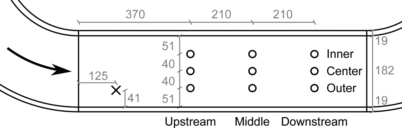
Fig. 10. Locations of the wind profiles (![]() ) in the main test section. The reference location of the MiniAir (
) in the main test section. The reference location of the MiniAir (![]() ) is 10 cm below the ceiling. The dimensions are given in mm. The sketch is not to scale.
) is 10 cm below the ceiling. The dimensions are given in mm. The sketch is not to scale.
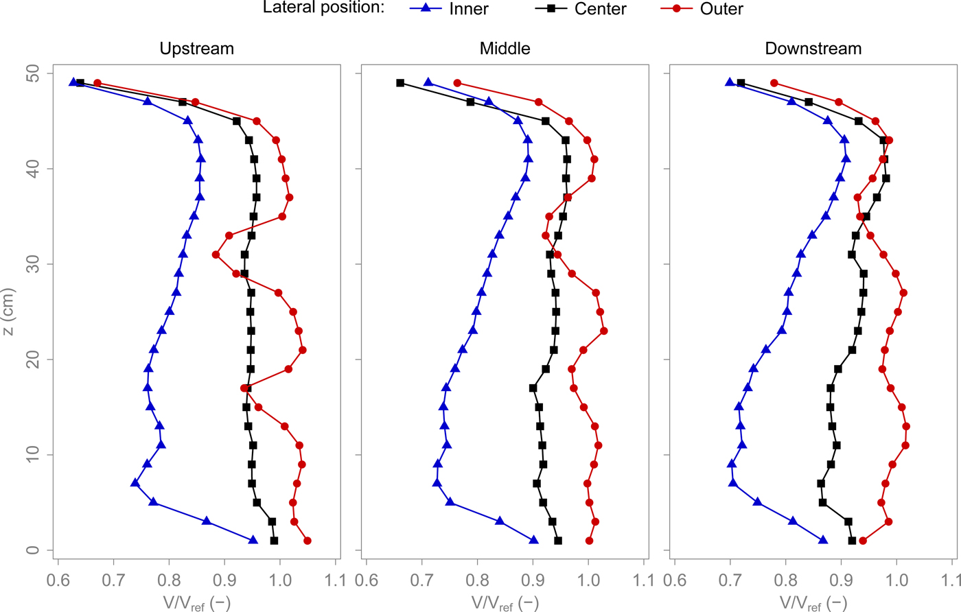
Fig. 11. Vertical profiles of normalized wind speed. z is the height above the wooden floor. The reference wind speed V ref is the wind speed measured in the usual position of the MiniAir. V ref was 3 m s−1. Figure 10 shows the locations of these profiles.
A3. DISCUSSION
The idea behind the new wind tunnel was to simulate an infinite fetch. This could not be fully achieved. The snow surface did not remain uniform during drifting snow events. It appears that the propeller is the main cause for these irregularities. The use of a single wind source necessarily results in a flow which is not uniform. Simple simulations of the flow with ANSYS Fluent revealed that a jet forms behind the propeller, which then bends downwards and reaches the surface a certain distance downstream. Furthermore, there is an area with low wind speeds below the propeller. In the annular as well as in the obround wind tunnel, we always observed an accumulation below the propeller and strong erosion downstream of it. The simulations may not be very precise but the deposition/erosion patterns observed in the wind tunnel correspond well to the simulated jet and low-speed area. It must be concluded that a single propeller is not a suitable drive system to create an uniform flow in a closed-circuit wind tunnel. A more uniform flow could be achieved by moving the flow boundaries instead of the fluid, by either rotating the cover or both the channel and the cover (Krishnappan, Reference Krishnappan1993; Schmundt and others, Reference Schmundt, Münsterer, Lauer, Jähne, Jähne and Monahan1995). This comes at a price of complexity and practicality and is only possible with a circular channel. As a consequence, we used the wind tunnel similarly to a normal closed-circuit facility with most of the measurements being performed in the main test section. In the beginning, the propeller was placed just downstream of the main test section to allow for a maximum of flow settling. During drifting snow events, however, the deposition below the propeller propagated into the main test section. This is why the motor/propeller was moved downstream to its current location. With the motor in the old position, the wind profiles were quite different. For example, the wind speed close to the surface of the inner profiles was 40% lower than that of the outer profiles. This corresponds to our observations that there was much more drifting snow in the outer half-width than close to the inner wall. It was fortunate that moving the motor to its current position also lead to a more uniform wind speed across the width of the channel, as shown in Figure 11. The saltation intensity was fittingly observed to be much more uniform across the width of the channel. The wind profiles in Figure 11 sustain the assumption made in the beginning, that there is a large core flowing at the free stream velocity. Despite this, the estimates made in the design phase were not entirely correct. For example, the measured free stream velocity never exceeded 8 m s−1, whereas up to 10 m s−1 were expected. However, we rarely experimented with wind speeds above 7 m s−1 because the centrifugal effects simply became too strong. The wind profiles above snow may be different from those shown in Figure 11, even though the shape of the profiles is expected to be similar as long as the snow surface is flat. But uneven erosion and deposition patterns will certainly modify the flow conditions. So, the flow is neither steady nor uniform as it would ideally be in an infinite-fetch wind tunnel. Furthermore, our knowledge of the existing flow is limited to the large-scale flow features in the main test section. Therefore, we cannot make quantitative statements concerning the flow's effects on individual snow grains. This wind tunnel is not adapted to measure onset of saltation for example. However, the focus of this facility is on the bed material, how it reacts and how its properties change under the influence of wind, and not on the flow itself.


 Open access