


Impact Statement
Wind turbine wakes have detrimental effects on downstream turbines within a wind farm, such as increased fatigue loading and reduced power generation. Near the rotor, these wakes are characterized by the helical vortices shed from the tips of the blades. Accelerating the breakdown of these vortices can mitigate the negative wake effects by reducing the number of coherent flow structures and enhancing mixing with the surrounding flow. One way to induce this breakdown is to introduce an asymmetry to the rotor, triggering the pairing instability to which helical vortex systems are subject. Most industrial rotors such as wind turbines have three blades, making the vortex dynamics in their wakes highly complex. The current study introduces a simplified model to investigate the effectiveness of different types of rotor asymmetry (e.g. blade extension, blade deflection, pitch change) at accelerating vortex breakdown in such a complex system.
1. Introduction
Wind turbine wakes, characterized by reduced wind speed and increased turbulence, can have negative effects on downstream turbines when operating in a wind farm. The reduction in energy generation of turbines within the wake of an upstream turbine relative to those that are unwaked can be as high as 40 %, one of the largest sources of wind farm power loss (Reference Lee and FieldsLee & Fields, 2021). In addition, wakes lead to increased fatigue loading on downstream turbines (Reference Herges, Berg, Bryant, White, Pacquette and NaughtonHerges et al., 2018; Reference Kim, Shin, Joo and KimKim, Shin, Joo, & Kim, 2015; Reference Lee, Churchfield, Moriarty, Jonkman and MichalakesLee, Churchfield, Moriarty, Jonkman, & Michalakes, 2013). The near wake (within 1–4 rotor diameters; (Reference Göçmen, van der Laan, Réthoré, Diaz, Larsen and OttGöçmen et al., 2016; Reference Vermeer, Sørensen and CrespoVermeer, Sørensen, & Crespo, 2003)) is dominated by vortices shed from the tips of the turbine blades, which form helical filaments in the shear layer between the slower wake and the faster surrounding flow. The persistence of these coherent structures into the far wake can be responsible for further increases in fatigue loading on downstream turbines (Reference Lee, Churchfield, Moriarty, Jonkman and MichalakesLee et al., 2013; Reference SørensenSørensen, 2011).
As the wake propagates downstream, it begins to recover, re-energizing by mixing with the surrounding flow. However, Reference Lignarolo, Ragni, Scarano, Simão Ferreira and Van BusselLignarolo, Ragni, Scarano, Simão Ferreira, and Van Bussel (2015) showed that vortices shed from the blade tips of the rotor prevent this mixing, as they transport mean-flow kinetic energy both into and out of the wake at similar rates. Once these tip vortices break down, energy flux into the wake generated by random turbulent motion dominates, substantially speeding up the recovery process. Tip vortex breakdown is triggered by inherent instabilities in the helical vortex system, of which there are two types (Reference Brynjell-Rahkola and HenningsonBrynjell-Rahkola & Henningson, 2020; Reference Leweke, Quaranta, Bolnot, Blanco-Rodríguez and Le DizèsLeweke, Quaranta, Bolnot, Blanco-Rodríguez, & Le Dizès, 2014). One type, core instabilities, is caused by shortwave perturbations inside vortex cores (Reference Blanco-Rodríguez and Le DizèsBlanco-Rodríguez & Le Dizès, 2016, Reference Blanco-Rodríguez and Le Dizès2017; Reference Hattori and FukumotoHattori & Fukumoto, 2009). The second type, displacement instabilities, which involve shifting the entire vortex position, is the focus of the current study (Reference Gupta and LoewyGupta & Loewy, 1974; Reference Okulov and SørensenOkulov & Sørensen, 2007; Reference WidnallWidnall, 1972). Displacement instabilities can lead to pairing between adjacent vortices, a phenomenon which has been shown to play an important role in the breakdown of vortices shed from wind turbine rotors (Reference Lignarolo, Ragni, Scarano, Simão Ferreira and Van BusselLignarolo et al., 2015; Reference Sarmast, Dadfar, Mikkelsen, Schlatter, Ivanell, Sørensen and HenningsonSarmast et al., 2014), propellers (Reference Felli, Camussi and Di FeliceFelli, Camussi, & Di Felice, 2011) and helicopters (Reference Bhagwat and LeishmanBhagwat & Leishman, 2000). This pairing occurs when adjacent vortices group together and roll up around each other, analogous to the leapfrogging behaviour observed with parallel vortex rings (e.g. Lugt Reference Cheng, Lou and LimCheng, Lou, & Lim, 2015; Reference LugtLugt, 1996).
This leapfrogging instability can be triggered in the helical vortices in rotor wakes by dynamically perturbing the tip vortices. Reference Odemark and FranssonOdemark and Fransson (2013) used pulsed jets on the nacelle of a turbine model to experimentally replicate the numerical analysis of tip vortex instability conducted by Reference Ivanell, Mikkelsen, Sørensen and HenningsonIvanell, Mikkelsen, Sørensen, and Henningson (2010). The disturbance caused a reduction in tip vortex energy, though without a strong dependence on the forcing frequency. Reference Quaranta, Bolnot and LewekeQuaranta, Bolnot, and Leweke (2015) modulated the rotation frequency of a one-bladed rotor to trigger instabilities in the generated helical vortex at different wavenumbers, observing growth rates consistent with those calculated for the pairing of an array of point vortices. Reference Quaranta, Brynjell-Rahkola, Leweke and HenningsonQuaranta, Brynjell-Rahkola, Leweke, and Henningson (2019) extended this work to a two-bladed rotor, resulting in a system of two interlaced helices. In addition to the local pairing induced by changes in the rotor rotation speed, they observed global pairing between the two helices when an asymmetry was imposed on the rotor, triggering the zero-wavenumber instability mode. Taking a different approach, Reference Huang, Alavi Moghadam, Meysonnat, Meinke and SchröderHuang, Alavi Moghadam, Meysonnat, Meinke, and Schröder (2019) simulated the effect of oscillating rotor blade trailing edge flaps on tip vortex formation and displacement. The perturbation was observed to grow at a similar rate as that predicted by Reference Ivanell, Mikkelsen, Sørensen and HenningsonIvanell et al. (2010) for the same wavenumber, and led to vortex pairing and breakdown. Similarly, Reference Marten, Paschereit, Müller and OberleithnerMarten, Paschereit, Müller, and Oberleithner (2020) simulated the actuation of trailing edge flaps over a range of frequencies. They successfully induced vortex pairing using this method and found that, even under turbulent inflow conditions, a small actuation amplitude was sufficient to shift the wake breakdown location upstream significantly. Reference Brown, Houck, Maniaci, Westergaard and KelleyBrown, Houck, Maniaci, Westergaard, and Kelley (2022) used existing turbine control mechanisms (blade pitch and rotor speed) on a simulated turbine to modulate the wake at a range of frequencies, demonstrating a reduction in wake length.
Though the aforementioned studies have successfully demonstrated the potential of capitalizing on helical vortex instabilities to accelerate wake breakdown, all except Reference Quaranta, Brynjell-Rahkola, Leweke and HenningsonQuaranta et al. (2019) exclusively investigated dynamic perturbation methods. Passive flow control methods to trigger the pairing instability would remove the need for additional parts such as flaps or increased wear on existing turbine components such as pitch mechanisms. They also avoid the additional energy consumption required to actuate active control methods. A wide variety of passive flow control methods for wind turbine blades have been proposed (Reference Aramendia, Fernandez-Gamiz, Ramos-Hernanz, Sancho, Lopez-Guede and ZuluetaAramendia et al., 2017), most of which focus on improving the lift-to-drag ratio of the airfoils. Reference Quaranta, Brynjell-Rahkola, Leweke and HenningsonQuaranta et al. (2019), however, used a slight rotor asymmetry as a form of passive flow control to trigger global vortex pairing, with the objective of accelerating wake breakdown. When extending such an investigation to a three-bladed rotor, the configuration typically used for utility-scale wind turbines, the complexity of the interlaced helical vortex system in the wake increases significantly. Because of this increased complexity, a simplified model is needed to establish a more complete understanding of the behaviour of the three-vortex system.
The focus of the current work is the development of such a simplified model to investigate the effect of rotor asymmetry on the wake of a three-bladed rotor. Reference WidnallWidnall (1972) studied the stability of a single helical vortex filament, including the effects of the entire filament on the self-induced velocity. Extending this work, Reference Gupta and LoewyGupta and Loewy (1974) calculated the instability growth rates of multiple interdigitated helices. Reference Quaranta, Bolnot and LewekeQuaranta et al. (2015) compared the growth rates obtained by Reference Gupta and LoewyGupta and Loewy (1974) with those predicted for two-dimensional point vortices (Reference LambLamb, 1932), demonstrating strong similarities between the two configurations. This comparison was then refined by Reference Quaranta, Brynjell-Rahkola, Leweke and HenningsonQuaranta et al. (2019) by applying the analysis of three-dimensional arrays of straight vortices conducted by Reference Robinson and SaffmanRobinson and Saffman (1982) to the investigation of instabilities of different wavenumbers in a two-helix system. The agreement between these different geometries showed that, for helical vortex systems with a moderate pitch, pairing between adjacent vortices is the underlying mechanism governing displacement instabilities. Reference Delbende, Selçuk and RossiDelbende, Selçuk, and Rossi (2021) conducted a thorough exploration of simplification methods for the analysis of two interlaced helices that are perturbed such that helical symmetry is preserved, i.e. with the zero-wavenumber mode. They demonstrated that a point vortex representation of the helices provides insight into the vortex dynamics, and the pairing behaviour in particular, for cases with low helical pitch. For intermediate pitch values, an array of vortex rings better represents the helical vortex system. At the largest pitch values, the effectiveness of an inviscid helical filament approximation was investigated.
The current study focuses on the low- to moderate-pitch range, relevant to industrial rotor wakes such as wind turbines and helicopters, where the point vortex approximation is expected to represent the helical vortex system with sufficient accuracy. This model is used to capture the effects of the zero-wavenumber instability mode which triggers global vortex pairing, induced by rotor asymmetry. Because of the relative simplicity of the point vortex approximation, the intricate nonlinear dynamics of the three-vortex system can be explored. Such an investigation can shed light on the behaviour of perturbed wakes of wind turbines, helicopters and propellers. In addition, it can help elucidate the occurrence of vortex pairing previously observed in laboratory experiments, but never fully explained (e.g. Reference Alfredsson and DahlbergAlfredsson & Dahlberg, 1979; Reference Felli, Camussi and Di FeliceFelli et al., 2011; Reference Sherry, Nemes, Lo Jacono, Blackburn and SheridanSherry, Nemes, Lo Jacono, Blackburn, & Sheridan, 2013; Reference Whale, Anderson, Bareiss and WagnerWhale, Anderson, Bareiss, & Wagner, 2000). The article is organized as follows. Section 2 describes the simplified point vortex model used to represent the helical vortex dynamics. Section 3 presents the validation of the model using a helical filament model and water channel experiments. In § 4, the results of the application of the model are presented. Finally, § 5 provides a summary of key findings and conclusions of the study.
2. Point vortex model
Consider a system of  $N$ interlaced helical vortex filaments in a cylindrical coordinate system $(r, \theta, z)$. The helices have the same radius, $R$, and helical pitch, $h'$, and $h=h'/N$ is the separation between neighbouring vortex loops in the axial $z$-direction. The unperturbed vortex positions are defined as
 \begin{equation} \boldsymbol{r}_\alpha = \begin{pmatrix} r_\alpha \\ \theta_\alpha \\ z_\alpha \end{pmatrix} = \begin{pmatrix} R \\ \theta + 2 {\rm \pi}\alpha/N \\ h'\theta/(2{\rm \pi}) \end{pmatrix}, \end{equation}
where  $\alpha$ is the helix index from 1 to $N$. The developed plan view of such a helical vortex system with $N = 3$ is shown in figure 1(a), appearing as a periodic array of inclined straight vortices. In two dimensions, this straight vortex array is represented by a periodically repeating strip of point vortices in the plane indicated by the dashed line in the figure. In this plane, the spacing between vortices is $b$, rather than $h$, which can be computed from the array geometry as $b=2{\rm \pi} Rh/L$. Note that the angle of the vortices, $\varphi$, in figure 1(a) is exaggerated for clarity, but in the helical vortex systems of interest here where $h/R$ is small, $\varphi \approx 80^{\circ }$ and $b\approx 0.97h$.

Figure 1. (a) Developed plan view of a helical vortex system with  $N=3$. Key geometric parameters are labelled. A perpendicular plane intersecting along the dashed line yields a periodic strip of point vortices, where the $x$-direction is indicated in the figure and the $y$-direction is out of the plane. (b) Point vortex trajectories in the plane perpendicular to that in (a) for the case where one of the three vortices (grey) is displaced in the $+y$-direction, as indicated by the black arrow on the base strip. The dashed line along $y/b=0$ corresponds to the dashed line in (a). The intensity of the colours represents time, with darker intensities indicating larger values. The open circles show the initial positions of the vortices and the filled circles mark their positions at dimensionless time $t^*=t\varGamma /(2h^2)=4$. (c) The interlaced helices reconstructed from the point vortex evolution. The lighter coloured sections on the left-hand side (blue and red) represent the parts of the helices that are extended backwards from the start of the point vortex evolution to connect to the rotor.
The dynamics of the two-dimensional, periodic strip of  $N$ point vortices repeated infinitely along the $x$-axis can be described using the following formula (Reference ArefAref, 1995):
 \begin{equation} \frac{{\rm d}\zeta^ * _\alpha}{{\rm d} t} = \frac{1}{2Nbi} \sum_{\beta = 1\atop \beta \neq \alpha}^{N}\varGamma_\beta \cot\left\{\frac{\rm \pi}{Nb}(\zeta_\alpha - \zeta_\beta)\right\}, \end{equation}
where  $\zeta _\alpha = x_\alpha +iy_\alpha$ is the complex position of the point vortex $\alpha$; $\varGamma _\alpha$ is its circulation; and $*$ represents the complex conjugate. In the two-dimensional coordinate system shown in figure 1(b), the $x$ direction corresponds to the direction along the dashed line in figure 1(a) and the $y$-direction is perpendicular to the plane in figure 1(a). In a system of identical, evenly spaced point vortices, none of the vortices will move. However, the system is unstable, so any perturbation (i.e. displacement in $x$ or $y$, change in circulation) will cause the vortices to move along intertwining trajectories such as those shown in figure 1(b) for the case of the displacement of one vortex in the $+y$-direction.
After determining the trajectories of the point vortices in the  $x$–
$x$– $y$ plane, the helical system can be reconstructed (figure 1c). Such reconstruction is performed by converting the temporal evolution of the basic strip of $N$ vortices into the spatial evolution of the helical geometry using the helical advection speeds in the azimuthal and axial directions. In the case of a rotor wake, these speeds are determined by the rotor rotation speed $f$, with the advection speed $u_\theta = 2{\rm \pi} f$ in the azimuthal direction and $u_z = h'f$ in the axial direction. At each time step, the vortex advances along the helical path determined by $u_\theta$ and $u_z$, with additional displacement caused by the perturbation. The perturbation-induced displacement in the $y$-direction becomes a radial displacement in the helical coordinate system, while the $x$-displacement is projected into the axial and azimuthal directions, with the majority in the axial direction due to the small value of $\varphi$:
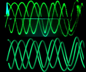
 \begin{equation} \begin{pmatrix} \delta r_\alpha \\ \delta \theta_\alpha \\ \delta z_\alpha \end{pmatrix} = \begin{pmatrix} \delta y_\alpha \\ \delta x_\alpha \text{cos}(\varphi) \\ \delta x_\alpha \text{sin}(\varphi) \end{pmatrix}. \end{equation}
 As figure 1(a) shows, the initial positions of the vortices in the point vortex model (along the dashed line) are not the same as the initial positions of the vortices shed from the rotor at  $z=0$. Therefore, a decision must be made about how to connect the vortices to the rotor. Because the motion of each vortex is strongly influenced by the induced velocity from its neighbours, the point vortices in the model are ‘released’ once all three have been shed from the rotor. The first and second vortex (blue and red in the figure) are then extended back along the helical trajectory to the rotor. These extended regions of the helices are indicated by lighter colouring in figure 1(c).
3. Model validation
The point vortex model uses a highly simplified approach to solve for the dynamics of helical vortices, neglecting the effects of curvature, core size and spatial evolution. To determine if the model produces useful results in spite of these simplifications, it is validated against a more sophisticated filament model and a series of experiments conducted in a water channel on the helical vortices in the wake of a rotor.
3.1 Filament model
The vortex filament model used for validation was first introduced by Reference Leishman, Bhagwat and BagaiLeishman, Bhagwat, and Bagai (2002) for the description of rotor wakes. The numerical code used here has been developed and described in detail by Reference Durán Venegas and Le DizèsDurán Venegas and Le Dizès (2019), Reference Castillo-Castellanos, Le Dizès and Durán VenegasCastillo-Castellanos, Le Dizès, and Durán Venegas (2021) and Reference Durán Venegas, Rieu and Le DizèsDurán Venegas, Rieu, and Le Dizès (2021). It employs a Lagrangian description of vortices with small core sizes, which are discretized into straight segments. In this model, vorticity is concentrated along material lines which are advected by the local velocity field, as follows:
 \begin{equation} \frac{{\rm d}\boldsymbol{r}_\alpha}{{\rm d} t} = \boldsymbol{u}_{BS}(\boldsymbol{r}_\alpha) + \boldsymbol{u}_{0}, \end{equation}
where  $\boldsymbol {u}_{BS}$ is the induced velocity calculated using the Biot–Savart law for filaments and $\boldsymbol {u}_{0}$ is an external flow field. The filament approach is first used to model three infinite interlaced helices to introduce the effects of curvature and core size, which are not included in the point vortex model. In this case, $\boldsymbol {u}_{0}=0$ and the reference frame is defined to follow a vortex particle along the unperturbed helix. One of the helices is perturbed with a radial expansion of $\delta r_1 = 0.05h$ to compare with a $y$-displacement of the same magnitude applied to one of the vortices in the point vortex model. This deformation is uniform, and the perturbation evolves in time according to (3.1).
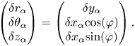
In figure 2, the trajectories of the vortices in the point vortex model are compared with those from the filament model for a constant core radius of  $a/R=0.01$ and different values of the helix geometrical parameter, $h/R$. The evolution of the $x$-positions over time is shown in figure 2(a), while the $y$-positions are shown in figure 2(b). In the chosen filament model reference frame, the unperturbed vortex system is stationary and the only motion comes from the perturbations. Time is non-dimensionalized by the relevant time scale for longwave instability evolution (Reference Quaranta, Bolnot and LewekeQuaranta et al., 2015), such that $t^*=t\varGamma /(2h^2)$. These trajectories show that the point vortex model successfully reproduces the vortex trajectories from the higher-fidelity filament model for the first several time units. Around $t^*=8$, the trajectories deviate more significantly, with the $y$-position of two of the vortices in the point vortex model switching relative to the filament model. However, it should be noted that in most real-world situations, the beginning of the vortex evolution is most relevant as the vortices begin to break down as they interact. The effect of helix geometry is also observed in the improved agreement of the point vortex model with the filament model for $h/R=0.10$ compared with $h/R=0.33$. As $h/R$ decreases, the curvature of the filaments decreases relative to the pitch, and the geometry more closely resembles an array of straight filaments represented by point vortices. Reference Delbende, Selçuk and RossiDelbende et al. (2021) conducted a similar comparison for a perturbed pair of helical vortices, showing that point vortices provide a good approximation for their behaviour when $h/R$ is sufficiently small, typically for $h/R\lesssim 0.3$. Dependence on core size is discussed in detail below.
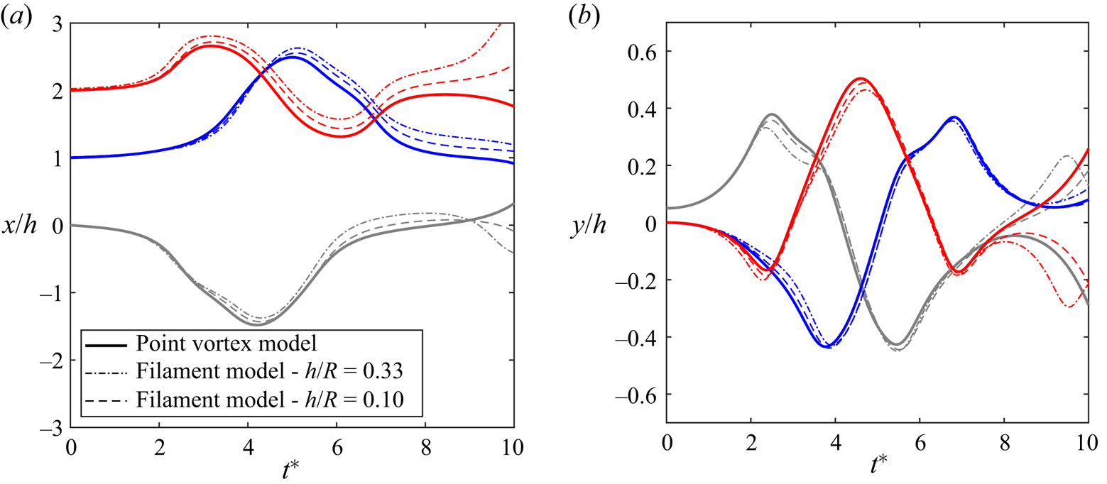
Figure 2. Comparison between vortex trajectories predicted by the point vortex model and filament model for two different values of  $h/R$ and constant core radii of $a/R=0.01$, including (a) the $x$-component and (b) the $y$-component.
Next, in order to evaluate the accuracy of the transformation from temporal to spatial evolution employed in the point vortex model, spatially evolving helices are modelled using the filament method. As described in Reference Durán Venegas, Rieu and Le DizèsDurán Venegas et al. (2021), the spatially evolving filament method models helical vortices in the laboratory reference frame with external velocity
 \begin{equation} \boldsymbol{u}_{0} = \begin{pmatrix} 0 \\ 0 \\ U_0 \end{pmatrix}, \end{equation}
such that the helices rotate as they would when shed from a rotor. Vortices are prescribed at the rotor plane and match uniform helices in the far field, which enables the inclusion of radial expansion observed near the rotor plane. From this baseline state, one of the vortices is perturbed in the radial direction by  $\delta r_1$ at the rotor plane. The perturbations then propagate downstream and modify the wake structure and induced velocity accordingly. Qualitatively, the reconstructed wakes from the point vortex model agree well with those from the filament method, with the most visible difference due to the slight radial expansion ( ${\sim }10\,\%$ of $R$) in the filament model, which is not included in the point vortex model. The quantitative metric used to compare the filament model with the point vortex model is the location where leapfrogging (or vortex swapping) occurs, $z_s$, shown by Reference Quaranta, Brynjell-Rahkola, Leweke and HenningsonQuaranta et al. (2019) to be an effective indicator of the evolution speed of the instability. In both the filament and point vortex models, $z_s$ is defined as the point where the $\theta$ and $z$ positions of two of the vortices are equal, i.e. the point where one loop of a helix passes over the one adjacent to it (figure 3a). Other metrics for evaluating the perturbation evolution were investigated and provided similar results, but leapfrogging distance was chosen because it can be identified easily in models and experiments, and it has been shown to be the point where vortex breakdown begins (Reference Lignarolo, Ragni, Scarano, Simão Ferreira and Van BusselLignarolo et al., 2015).

Figure 3. (a) Reconstructed helices from the point vortex model for the case with  $\eta =0.02$, $\lambda =5$ and $\delta r_1/h=0.17$, showing the definition of leapfrogging distance, $z_s$. (b) Comparison between $z_s/R$ computed using the point vortex model (PVM) and the spatially evolving filament model (FM) for a range of tip speed ratios ( $\lambda$) and dimensionless circulations ( $\eta$) with a constant initial perturbation of $\delta r_1/h=0.05$ and core radii of $a/R=0.02$. (c) The effect of the initial perturbation magnitude on the two models for varying $\delta r_1/h$, with $\eta =0.02$, $\lambda =5$ and $a/R=0.02$. The black dashed and dashed–dotted lines represent the least-squares fit of the point vortex model and filament model results to $z_s/R=c_1-c_2 \text {ln}(\delta r_1/h)$, respectively. (d) Subset of $\delta r_1/h$ values from (c) showing the effect of changing core radius, $a/R$.
The results of the spatially evolving filament model are compared with those of the point vortex model for a range of parameters. Figure 3(b) shows the dependence of  $z_s$ on tip speed ratio, $\lambda =2{\rm \pi} f R/U_0$, and dimensionless circulation, $\eta =\varGamma /(2 {\rm \pi}f R^2)$, which control the spacing and strength of the vortices, respectively. The radial perturbation and core radii are held constant at $\delta r_1/h=0.05$ and $a/R=0.02$. As $\lambda$ increases, the instability evolves faster and $z_s$ decreases, consistent with the experimental results of Reference Quaranta, Brynjell-Rahkola, Leweke and HenningsonQuaranta et al. (2019) for two vortices. Both the filament model and the point vortex model capture this trend, though the point vortex model underpredicts $z_s$ slightly at large values of $\lambda$ and overpredicts $z_s$ slightly for small $\lambda$. The instability also evolves more quickly for larger values of $\eta$, as is expected for increasing vortex strength. This trend is captured with remarkably good agreement by both models. The effect of initial perturbation magnitude is investigated in figure 3(c), shown for a typical set of helix parameters where $\eta =0.02$, $\lambda =5$ and $a/R=0.02$. The instability evolves faster as the perturbation magnitude increases, with steeper growth at lower values of $\delta r_1$, following the logarithmic relationship proposed by Reference Quaranta, Brynjell-Rahkola, Leweke and HenningsonQuaranta et al. (2019): $z_s/R=c_1-c_2 \ln (\delta r_1/h)$ where $c_1$ and $c_2$ are constants for given values of $\eta$ and $\lambda$. For all values of $\delta r_1$, the point vortex model does an excellent job of predicting the leapfrogging distance computed by the more sophisticated filament model.
Figure 3(d) shows the effects of varying the core radius used in the filament model,  $a/R$, over 2.5 orders of magnitude. Decreasing the core size reduces the value of $z_s/R$, indicating that smaller vortex cores cause the perturbation to evolve faster. This trend is likely related to the relationship between core size and the self-induced velocity of a helical vortex along the $z$-direction, which increases as $a/R$ decreases. One might expect, therefore, that the values of $z_s/R$ predicted by the point vortex model would be larger than those obtained using the filament model for all values of $a/R$, because self-induced velocity is not included in the point vortex model. However, the good agreement between the point vortex and filament models for intermediate values of $a/R$ suggests that the self-induced velocity is balanced by another effect that acts to slow the evolution of the perturbation and which is not included in the point vortex model. It is proposed that the finite spatial extent of the vortices in the spatially evolving filament model slows the perturbation evolution relative to the infinite extent represented by the point vortex model. There are no vortices upstream of the rotor inducing additional velocities in the wake, whereas in the point vortex model, an infinite number of vortices in both directions exert their influence on the vortex dynamics.
The core size effect is much weaker than the effects of tip speed ratio, vortex circulation or perturbation magnitude, such that an order of magnitude change in  $a/R$ only reduces $z_s/R$ by approximately 8 %. This relatively weak dependence is consistent with the findings of Reference Delbende, Selçuk and RossiDelbende et al. (2021). The results presented in Figure 3(d) indicate that the point vortex model captures the perturbation evolution most effectively when the core radius is of the order of $10^{-2}R$. This order of magnitude is realistic for typical industrial rotor geometries. Reference Okulov and SørensenOkulov and Sørensen (2010) estimated that the core size asymptotes to $h/(18R)$ for three-bladed Joukowsky wind turbine rotors with small values of $h/R$. Reference Segalini and AlfredssonSegalini and Alfredsson (2013) calculated core sizes of $a/R=0.047$ for an experimentally tested four-bladed propeller and $a/R=0.033$ for a simulated three-bladed 2 MW wind turbine. Core sizes for the MEXICO experimental wind turbine rotor were measured to be $a/R\sim 0.01$ (Reference Nilsson, Shen, Sørensen, Breton and IvanellNilsson, Shen, Sørensen, Breton, & Ivanell, 2015). In the experimental campaign discussed in the following section, the core size was measured as $a/R=0.01$ and $a/R=0.02$ for the two- and three-bladed model rotors, respectively. Therefore, comparison with the filament model indicates that the point vortex model can be used confidently for most real-world applications.
3.2 Water channel experiments
The point vortex model is also validated experimentally using two- and three-bladed rotors in a recirculating free-surface water channel to generate helical tip vortices. Some of the two-bladed rotor results were presented by Reference BolnotBolnot (2012) and Reference Quaranta, Brynjell-Rahkola, Leweke and HenningsonQuaranta et al. (2019) and are now used to compared with the results of the point vortex model, while the three-bladed rotor results are new. The experimental set-up for the two-bladed rotor is described in detail by Reference BolnotBolnot (2012) and Reference Quaranta, Brynjell-Rahkola, Leweke and HenningsonQuaranta et al. (2019). The set-up for the three-bladed rotor is the same, with the exception of the rotor design. The water channel used for both sets of experiments has a test section with dimensions  $150\,{\rm cm} \times 38\,{\rm cm}\times 50\,{\rm cm}$ (length $\times$ width $\times$ height). The rotors used to generate helical vortices are mounted on a shaft with a 1.5 cm diameter extending 96 cm downstream, with a bearing for support at the midpoint of the shaft. The rotation is driven by a stepper motor outside of the water, connected to the shaft through a gearbox. The rotor wake, including vortex properties, is measured using particle image velocimetry (PIV) (see supplementary material available at https://doi.org/10.1017/flo.2022.33), and the vortices are visualized using fluorescent dye painted on the blade tips.
The two-bladed rotor has a radius of  $R=8$ cm and an A18 airfoil cross-section (Reference Selig, Guglielmo, Broeren and GiguèreSelig, Guglielmo, Broeren, & Giguère, 1995). It is milled from a single piece of aluminium. The vortex system is perturbed by introducing a slight radial offset of the rotor, $\delta r$, such that the radial position of the first blade tip is $R-\delta r$ and the second is $R+\delta r$. Two sets of experiments were conducted on the two-bladed rotor, the first with varying tip speed ratio, $\lambda$, and constant $\delta r/R$ (presented in Reference Quaranta, Brynjell-Rahkola, Leweke and HenningsonQuaranta et al. (2019), and the second with constant $\lambda$ and varying $\delta r$. In both sets of experiments, the axial position of vortex leapfrogging, $z_s$, is used as a metric for quantifying the evolution of the instability in comparison with the results of the point vortex model. To compare with the experiments, the point vortex model uses the experimental values of vortex circulation and helical pitch as inputs, obtained from PIV measurements (see supplementary material). As shown in figure 4, the point vortex model predicts well the leapfrogging location observed in the experiments. In the set of experiments where $\lambda$ is varied, small deviations are observed at individual $\lambda$ values, whereas in the set where $\delta r$ is varied, the model consistently underpredicts $z_s$ by approximately 8 %. This discrepancy suggests that the point vortex model slightly overestimates the strength of the interaction between the vortices, causing the instability to evolve faster. This overestimation could be related to the change in vortex spacing that occurs in the experiment. As reported by Reference Quaranta, Brynjell-Rahkola, Leweke and HenningsonQuaranta et al. (2019), $h/R$ decreases slightly with downstream distance until levelling off at $h_\infty$, which is the value used for the spacing in the point vortex model. The larger spacing at the beginning may cause the perturbation to evolve more slowly in the experiment. Still, the model accurately captures the trends observed in the experiments, and the error is small considering the simplicity of the model.

Figure 4. (a) Comparison between (top) an experimentally obtained dye visualization of the tip vortices in the wake of a two-bladed rotor, reproduced from Reference Quaranta, Brynjell-Rahkola, Leweke and HenningsonQuaranta et al. (2019), and (bottom) a two-vortex helix reconstructed using the point vortex model. The white arrow indicates the leapfrogging distance,  $z_s$. Comparison between the effect of (b) $\lambda$ and (c) $\delta$ on $z_s/R$ in the experiment and in the point vortex model.
The three-bladed rotor has a radius of  $R=9$ cm and a NACA2414 airfoil cross-section, with blade chord and twist designed to approximate a Glauert rotor for the outer 50 % of the radius (Reference GlauertGlauert, 1935). The rotor is operated at a tip speed ratio of $\lambda =3$ ( $\,f=3$ Hz, $U_0=56.0$ cm s $^{-1}$) to ensure sufficient spacing between adjacent helix loops. For higher values of $\lambda$, the helical pitch decreases, pushing the vortices closer together and leading to shortwave instabilities that mask the effects of the longwave instabilities which are the focus of the current study. With a tip chord of $c_{{tip}}=2.3$ cm, the tip chord-based Reynolds number is $Re=2{\rm \pi} f R c_{{tip}}/\nu \approx 40\,000$. These parameters lead to a tip vortex circulation of $\varGamma = 165 \pm 3\,\text {cm}^2\,\text {s}^{-1}$ and a helical pitch of $h=4.72 \pm 0.09\,\text {cm}$ for the baseline symmetric rotor, based on PIV measurements of the wake (calculation details in the supplementary material). Each blade is attached to the rotor hub individually, so one or two can be removed and replaced with a different geometry (e.g. radial extension, axial deflection) to introduce an asymmetry to the rotor.
In the example presented in figure 5, one blade is longer than the other two by  $\delta r_1/h=0.08$. In figure 5(a), the dye visualization of the vortices from the experiment is compared with the reconstructed helical vortices from the point vortex model, with the measured values of $\varGamma$ and $h$ as inputs. Qualitatively, it is clear that the model reproduces the vortex behaviour very well. For a more quantitative comparison, the axial and radial components of the vortex trajectories are plotted in figures 5(b) and 5(c), respectively. Both components are plotted against dimensionless time, $t^*=t \varGamma /(2h^2)$. The measured and modelled distance and dimensionless time to leapfrogging are shown in figure 5(b), and are related by $z_s=t^*_s(2h^2)u_z/\varGamma$, where $u_z=h'f$ as defined in § 2. Though $z_s$ can be more easily identified from the experimental dye visualizations, $t^*_s$ is more general because it is independent of the advection speed of the specific system. Predicting the advection speed for a given system is not straightforward, as it requires precise knowledge of the rotor induction or measured values of $h$ or $\varGamma$. Therefore, future analyses will use $t^*_s$ as a metric for perturbation effectiveness.
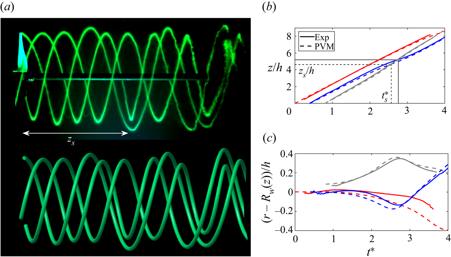
Figure 5. (a) Comparison between (top) an experimentally obtained dye visualization of the tip vortices in the wake of a three-bladed rotor and (bottom) a three-vortex helix reconstructed using the point vortex model, for  $\delta r_1 = 0.08h$. The white arrow indicates the leapfrogging distance, $z_s$. Comparison between the (b) $z$- and (c) $r$-components of the three vortex trajectories obtained from the experiment (Exp) and the model (PVM), with radial wake expansion ( $R_w$) removed. The three different line colours represent the trajectories for each of the three vortices, with the grey line corresponding to the perturbed vortex. The black solid and dashed lines in (b) mark the values of dimensionless leapfrogging time ( $t^*_s$) and distance ( $z_s/h$) for the experiment and the model, respectively.
The experimental trajectories presented in figure 5(b,c) represent the average position of 55 vortices taken from images of a wake cross-section below the shaft. In general, the vortex trajectories from the model agree well with those measured in the experiment, with only a slight upstream shift in leapfrogging position predicted by the model, consistent with the results for the two-bladed rotor presented in figure 4(c). In the radial direction, wake expansion that occurs in the experiment due to the velocity deficit in the wake,  $R_w(z)$, is subtracted from the trajectories. The discrepancy between the trajectories from the experiments and those from the point vortex model appears larger in the radial direction, primarily due to the smaller range of the vertical axis in the figure. This deviation is related to the experimental effects of wake expansion and blockage, which cannot be captured by the point vortex model. Though $R_w(z)$ is subtracted from the radial coordinate of the trajectories, it may have some secondary effects on the vortex dynamics that cannot be removed by this simple correction. For example, $h$ is relatively independent of axial position, but it deviates by ${\sim }6$% within $z/R<1$ (see supplementary material). Since $h$ strongly influences the vortex dynamics and small differences at the beginning of the evolution are amplified by the nonlinearity of the system, even such a small variation could affect the trajectories. Water channel blockage has also been shown to restrict wake expansion and radial motion of pairing vortices behind a model rotor when the blockage ratio, $B=A_{{swept}}/A_{{channel}}$ where $A_{{swept}}={\rm \pi} R^2$ is the swept area of the rotor and $A_{{channel}}$ is the cross-sectional area of the channel, is greater than 10 % (Reference McTavish, Feszty and NitzscheMcTavish, Feszty, & Nitzsche, 2014). For the three-bladed rotor configuration used in the experiment, $B=13$%, so blockage effects will influence the vortex motion. Note that $h/R=0.52$ for this rotor, which is larger than the value of $h/R\sim 0.3$ proposed as the limit of validity for the point vortex representation by Reference Delbende, Selçuk and RossiDelbende et al. (2021). Still, the point vortex model is shown here to capture the helical vortex dynamics exhibited in the experiment with remarkably good agreement.
4. Results and discussion
The point vortex model does not account for effects such as core size, curvature or even spatial evolution, i.e. the fact that the downstream vortices in a rotor wake are not exact copies of the base strip and there are no vortices upstream of the rotor. Nevertheless, good agreement is observed between its results and those of the filament model and experiments, highlighting the effectiveness of the point vortex model despite its simplicity. Such agreement suggests that this model balances the lack of self-induction related to curvature and core size with the additional influence of the velocity induced by the infinite vortex copies. This balance holds true for ranges of helical pitch and core size that are relevant for industrial applications, i.e.  $h/R\lesssim 0.5$ and $a/R\sim 10^{-2}$. After such successful validation of the model, it can now be used to gain insight into the expected behaviour of vortices in the wake of an asymmetric three-bladed rotor with various configurations.
4.1 Effect of perturbation direction
First, a parameter sweep of the displacement of a single vortex is conducted. Perturbation magnitudes between  $0$ and $0.07h$ are tested, with components in the radial and axial directions. Note that an azimuthal displacement of $\delta \theta$ would be equivalent to an axial displacement of $\delta z = 3h/(2{\rm \pi} ) \delta \theta$ because one helix extends $3h$ in the axial direction over one full rotation of $2{\rm \pi}$. Azimuthal and axial perturbations are two different methods for displacing a vortex along this helical trajectory. Because of this equivalence, azimuthal perturbations are not explored in detail. As explained in § 3.2, the dimensionless time to leapfrogging, $t^*_s$ (illustrated in figure 5b), is now used to quantify the effectiveness of the perturbations studied, as it is more general than $z_s$ which depends on the advection speed of the vortices. The map of $t^*_s$ presented in figure 6(a) shows that an increase in magnitude of the initial perturbation decreases the time to leapfrogging, indicating a faster evolution of the instability. Cross-sections along the diagonals of this map shown in figure 6(b) highlight the divergence of $t^*_s$ as the perturbation amplitude approaches 0. At the point where $\delta r_1 = 0$ and $\delta z_1 = 0$, $t^*_s$ is infinite because the vortices will never move. However, even very small values of $\delta$ can trigger large changes in the vortex behaviour, providing a possible explanation for the observation of leapfrogging in so many previous experimental studies (e.g. Reference Alfredsson and DahlbergAlfredsson & Dahlberg, 1979; Reference Felli, Camussi and Di FeliceFelli et al., 2011; Reference Sherry, Nemes, Lo Jacono, Blackburn and SheridanSherry et al., 2013; Reference Whale, Anderson, Bareiss and WagnerWhale et al., 2000).

Figure 6. (a) Map of dimensionless leapfrogging time ( $t^*_s$) for a range of initial perturbations of the position of one vortex. (b) Cross-sections of the map in (a) along the two diagonals where the magnitudes of $\delta z_1/h$ and $\delta r_1/h$ are equal. Both diagonals are symmetric about $(0,0)$. Examples of the (top) reconstructed vortex system from the point vortex model and (bottom) experimental dye visualization of the tip vortices for (c) the case where one vortex is perturbed by $\delta r_1/h=0.05$ and $\delta z_1/h=0.05$ and (d) the case where one vortex is perturbed by $\delta r_1/h=0.05$ and $\delta z_1/h=-0.05$. The stars in (a) indicate the points chosen for the examples.
The direction of the perturbation is also observed to have a significant effect on the vortex dynamics. When  $\delta r_1$ and $\delta z_1$ have the same magnitude but opposite signs, a sharp peak in $t^*_s$ is predicted. Moving off of this line, $t^*_s$ drops off quickly, reaching a minimum when $\delta r_1$ and $\delta z_1$ have the same magnitude and sign. Figure 6(b) shows that leapfrogging takes more than twice as long to occur for perturbations along the $\delta r_1 = -\delta z_1$ diagonal compared with those along the $\delta r_1 = \delta z_1$ diagonal. Note that the $\delta r_1 = -\delta z_1$ diagonal also represents the point where the vortex grouping switches, such that a vortex perturbed to the right of this line will group with vortices downstream, while a vortex perturbed to the left of the line will group with vortices upstream. The effect of perturbation direction is related to the mutually induced strain in a system of corotating vortices. Reference Leweke, Le Dizès and WilliamsonLeweke, Le Dizès, and Williamson (2016) show that the positive and negative strain directions are at $45^{\circ }$ angles relative to the axis between neighbouring vortices, which is the $z$-direction in this case. A vortex perturbed along the negative strain direction will be pulled back towards its initial position, while a perturbation along the positive strain direction will be amplified. Theoretically, it may seem like a vortex system perturbed exactly along the negative strain direction would never reach leapfrogging, as it would simply return to its initial configuration. However, because the perturbation of the position of one vortex also slightly perturbs the strain field, the vortex displacement will always increase, even if very slowly.
To confirm this directional dependence experimentally, one of the three-bladed rotor blades is replaced first with a blade with a tip deflected downstream by  $\delta z_1=0.05h$ and extended radially by $\delta r_1=0.05h$. As seen in figure 6(b), the experimentally measured vortices follow the behaviour predicted by the point vortex model well. Then a blade with $\delta z_1=0.05h$ and $\delta r_1=-0.05h$ is installed on the rotor. In this case, the instability takes longer to develop and the leapfrogging occurs much farther downstream (figure 6c). Leapfrogging occurs earlier in the experiment than predicted by the point vortex model, likely due to some small perturbations to the experimental flow, possibly generated by the shaft support located just downstream of the field of view.
4.2 Effect of circulation
Next the effect of a circulation change of one of the vortices is explored. Figure 7(a) shows how  $t^*_s$ changes when the circulation of one vortex is increased or decreased by $\delta \varGamma _1$. From this plot, it is clear that decreasing the circulation of one vortex is significantly more effective at reducing the time to leapfrogging than increasing the circulation of one vortex. The point vortex trajectories in figures 7(b) and 7(c) elucidate the reason behind this difference. When the circulation of one vortex is increased (figure 7b), the other two rotate around the stronger one, and leapfrogging occurs when the three are aligned at the same $x$-position. The two equal-strength vortices must travel a distance of $b$ in the axial direction before $t^*_s$. When the circulation of one vortex is decreased (figure 7c), however, the other two rotate around each other, and leapfrogging occurs when the two equal strength vortices have travelled $b/2$. Because this distance is shorter, leapfrogging occurs earlier and $t^*_s$ is smaller. The more favourable case with $\delta \varGamma _1/\varGamma = -0.07$ was tested experimentally by replacing one of the three rotor blades with one that was pitched by $-1^{\circ }$ relative to the other two. The circulation of the vortex shed from the modified blade was confirmed to be 7 % lower than those shed from the other two blades using PIV measurements. Figure 7(d) compares the reconstructed helical vortex wake from the point vortex model with the experimentally visualized rotor wake. The experimental wake follows the predicted trajectories well. It should be noted that, though even a small-magnitude change in $\varGamma$ produces a large reduction in $t^*_s$, an equivalent magnitude change in vortex position leads to a lower value of $t^*_s$ for most perturbation directions. This comparison shows that circulation perturbations are less effective than displacement perturbations at triggering the pairing instability.

Figure 7. (a) Plot of dimensionless leapfrogging time ( $t^*_s$) for circulation perturbations of one vortex. Examples of vortex trajectories for cases where (b) the circulation is increased by 7 % and (c) decreased by 7 %, obtained using the point vortex model. The open circles show the initial positions of the vortices and the filled circles mark their positions at $t^*=4.5$. (d) Example of the (top) reconstructed vortex system from the point vortex model and (bottom) experimental dye visualization of the point vortices for the case where $\delta \varGamma _1/\varGamma =-0.07$. The blue star in (a) indicates the example shown in (b) and the red star indicates the example in (c,d).
4.3 Perturbing multiple vortices
Finally, the point vortex model is used to investigate the effects of perturbing multiple vortices. Note that perturbing all three vortices does not provide any additional information relative to perturbing two vortices, as a simple shift of the vortex strip would achieve the same result. The point vortex model can be used to test any combination of perturbations of multiple vortices. However, in the following analysis, a single configuration is selected as a culmination of the findings of the previous two sections. In this configuration, shown in figure 8 with perturbation magnitude exaggerated for clarity, one vortex is perturbed in the positive  $x$-direction and positive $y$-direction, and the adjacent one is perturbed in negative $x$-direction and negative $y$-direction. Based on the previous findings, this combination is expected to be highly effective at reducing leapfrogging time. Both vortices are perturbed along the most unstable direction, as discussed in § 4.1. In addition, they are both perturbed such that they follow the trajectory that minimizes $t^*_s$, as discussed in § 4.2. The effects of such a perturbation are shown in figure 8(b), for $(\delta r_2, \delta z_2) = (0.05h, 0.05h)$ and $(\delta r_3, \delta z_3) = (-0.05h, -0.05h)$. This configuration leads to the fastest instability evolution yet observed in the current study, with leapfrogging predicted to occur just $1.9R$ downstream of the rotor plane. An experimental wake visualization confirms the accuracy of the model once more. It should be noted that, due to the nonlinearity of the vortex system, the leapfrogging distance observed in the current configuration is still greater than half of that observed in the case where one blade was changed ( $z_s=2.7R$).
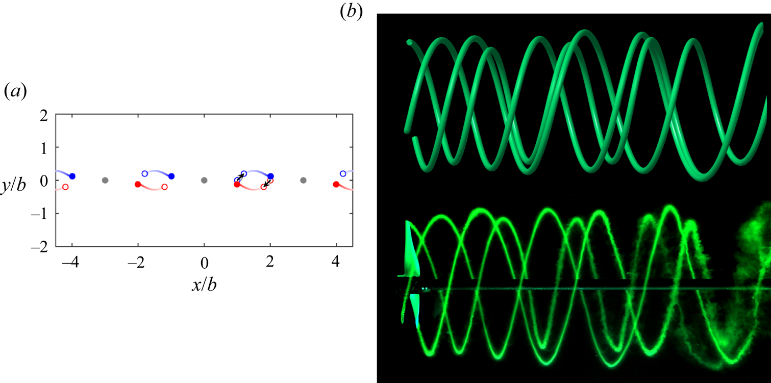
Figure 8. (a) Example of point vortex trajectories for the case where two vortices are perturbed along the unstable diagonal. The open circles show the initial positions of the vortices and the filled circles mark their positions at  $t^*=2$. The arrows indicate the perturbation on the base strip. (b) Example of the (top) reconstructed vortex system from the point vortex model and (bottom) dye visualization from the experiment for the case where $(\delta r_2, \delta z_2) = (0.05h, 0.05h)$ and $(\delta r_3, \delta z_3) = (-0.05h, -0.05h)$.
5. Conclusion
The current study introduces a simplified model for the analysis of asymmetric rotor wakes, which represents a helical vortex system as an infinitely repeating periodic strip of point vortices. Though such a representation does not account for the effects of vortex core size, curvature or spatial evolution, it is shown to accurately capture the helical vortex dynamics for industrially relevant ranges of helical pitch and core radius through validation against a more sophisticated filament model and water channel experiments on two- and three-bladed rotor wakes. The point vortex model is then used to provide insights into the types of perturbations that trigger the pairing instability most effectively, using the time to leapfrogging to quantify the speed of perturbation evolution. This metric is chosen because it can be identified easily in models and experiments, and previous work has shown that vortex breakdown and wake re-energizing begin after leapfrogging occurs in a wind turbine wake (Reference Lignarolo, Ragni, Scarano, Simão Ferreira and Van BusselLignarolo et al., 2015). Perturbing the vortex position along the direction of positive strain induced by corotating vortices is shown to cause the instability to evolve more quickly than displacing it by the same amount along the negative strain direction. When the circulation of one vortex is modified, a decrease is more effective than an increase, though both are less effective than a displacement. For all perturbations, increasing the magnitude reduces the time to leapfrogging. One case is investigated where two vortices are displaced, showing a further reduction in leapfrogging time.
The point vortex model has several advantages over more complex models. First, only a single equation (2.2) is required to determine the vortex dynamics. Such simplicity allows many different cases to be modelled and evaluated quickly. The model is also highly flexible in that the positions and circulations of all vortices in the system can be perturbed in any direction. In addition, it can be applied to a system with any number of vortices. Unlike linear stability analysis, the point vortex model can capture the nonlinear dynamics of the vortex motion for the zero-wavenumber mode. Most importantly, the model works well despite its simplicity. This effectiveness is due to a balance between the lack of self-induction which slows down the perturbation evolution and the presence of infinite vortex copies which speeds it up. This balance occurs when the values of helical pitch and core size are within a realistic range, with  $h/R\lesssim 0.5$ and $a/R\sim 10^{-2}$. However, even outside of these ranges, the qualitative trends and relative differences between different types of perturbations are expected to hold true.
The findings of the current study can be applied to the design of asymmetric rotors for industrial applications such as wind turbines. Currently, wind turbine rotors are highly symmetric due to a precise and repeatable manufacturing process. However, adding an asymmetry to the rotor design would perturb the helical vortex system in its wake, causing the coherent structures to break down. Since these structures contribute strongly to fluctuating loads on downstream turbines, rotor asymmetry has the potential to decrease the fatigue stress within a wind farm. In addition, such vortex breakdown leads to enhanced mixing between the low-energy flow in the wake and the high-energy flow outside, increasing the available energy for downstream turbines located in the wake. Though investigations into the practical considerations of asymmetric rotors under real-world conditions are underway, the results of the current study provide valuable guidance for how to proceed, particularly with regard to which configurations warrant further study. The current investigation shows that an asymmetry that displaces the blade tip along a favourable direction, e.g. through a combination of a length change and a deflection, can trigger the vortex instability most effectively. Changing two blades causes the instability to evolve faster than changing one blade, but the benefit is not doubled due to the nonlinearity of the system, which is important to note if the cost scales with the number of blades modified. Furthermore, the added asymmetry would only have to be 1 %–2 % of the rotor radius, as the instability evolution scales with vortex spacing, which is smaller relative to radius for a utility-scale wind turbine than for the model rotor used in the current study.
Supplementary material
Supplementary material is available at https://doi.org/10.1017/flo.2022.33.
Acknowledgements
The authors thank S. Le Dizès for helpful discussions and feedback on the manuscript.
Funding statement
This work was supported by the technology transfer company SATT Sud-Est (Marseille).
Declaration of interests
The authors declare no conflict of interest.
Data availability statement
Data and codes are available on request from the authors.


 Open access