


Introduction
The ice cap of Austfonna on Nordaustlandet in Svalbard is, at 8105 km2, one of the largest in the Northern Hemisphere outside the Greenland ice sheet (Fig. 1). A number of factors make Austfonna, and its component drainage basins, particularly suitable for glaciological modelling studies. Svalbard is at the present northern extremity of the warm North Atlantic Drift. As a result, the archipelago is particularly sensitive to climatic shifts, which have been reflected in past changes in ice extent and dynamics. Ice cores of 204 and 566 m have been obtained recently from Austfonna by Soviet glaciologists (personal communication from V. Zagorodnov). Analysis of these cores will provide data on mass-balance and temperature changes on the ice cap over the last few thousand years. Much of the eastern, tide-water margin of Austfonna is grounded below present sea-level, and is likely to be underlain by deformable sediments. Some basins within the ice cap have also been observed to surge, and Brȧsvellbreen has undergone the largest surge ever recorded (Reference SchyttSchytt, 1969). A detailed network of airborne radio echo-sounding is also available, showing that the subglacial topography of the ice cap is relatively simple (Reference DowdeswellDowdeswell and others, 1986). For

Fig. 1. Location map. a. Position of Austfonna within Nordaustlandet and the Svalbard archipelago. b. The surface topography of Austfonna contoured at 100 m intervals, with the ice divide defining Basin 5 indicated. Brȧsvellbreen (Br) is the large ice lobe on the south side of the ice cap. The point labelled “Is” is named Isdomen. c. Airborne radio echo-sounding flight lines superimposed on the ice divide defining Basin 5.
these reasons, Austfonna was selected for a detailed programme of glaciological field measurements and mathematical modelling of its present and past dynamic behaviour (Reference Drewry and LiestølDrewry and Liestøl, 1985; Reference DowdeswellDowdeswell, 1986a).
In this paper we report and discuss field measurements of several boundary conditions required in modelling studies of Austfonna. The parameters examined include ice-surface velocities and strain-rates, mass balance, and subglacial melt water. Field observations are concentrated in a drainage basin of about 670 km2 on the east side of the ice cap (Fig. 1), known as Basin 5 (Reference Dowdeswell and DrewryDowdeswell and Drewry, 1985). The ice-surface and bed morphology of this basin are also described in some detail. The results of (a) investigations of the thermal structure of Austfonna, and (b) finite-element and deformable subglacial layer modelling of Basin 5, together with their response to palaeoclimatic forcing, will be the subject of separate papers.

Fig. 2. Morphology of Basin 5, Austfonna: a. Ice surface; b. Bed. The location and identification letter or number of each stake and triangle within the trilateration network is shown. The airborne radio echo-sounding flight lines, on which surface and bedrock elevations are based, are located in Figure 1.c.
Data Sources and Methods
Velocities and strain-rates
Drainage Basin 5 extends approximately 30 km from the divide to the terminal ice cliffs (Fig. 1). To obtain measurements of ice-surface velocities and strain-rates, a network of 24 stakes was positioned within the basin (Fig. 2a). The stakes were arranged in two offset lines to form a series of triangles. Initial stake positioning was assisted by use of a satellite-navigation system, accurate to ±30 m. Each 5 m long aluminium pole was then frozen into a steam-drilled hole to a depth of 2–3 m. In the upper part of the basin, where ice-surface slopes were generally less than 1°, stakes were usually set 2–2.5 km apart. Towards the lower part of the network, distances between stakes were more normally 1–1.5 km. This ensured inter-visibility in what was an area of relatively rough ice-surface topography (Reference Dowdeswell and McIntyreDowdeswell and McIntyre, 1987). The network was orientated down the centre of the drainage basin, approximately parallel to the direction of maximum ice-surface slope. It was truncated, however, about 10 km from the tide-water margin of the basin due to increasingly heavy crevassing (Fig. 3).
After its emplacement, the trilateral network was surveyed in May 1986, and again during May 1987. The nearest bedrock outcrop to the network was 17 km distant, at Isispynten (Fig. 2), across severely crevassed ice. Point Y, located approximately at the ice divide, was therefore treated as fixed over the period of observation.

Fig. 3. Vertical aerial photograph of surface crevassing in the lower part of Basin 5, including the terminal ice cliffs (Norsk Polarinstitutt Id. No. S77 1213; 21 August 1977). The scale bar is 1 km.
Angular and distance measurements were taken using a Wild T-2 theodolite and DI-3000 electronic distance-measuring instrument (EDM). At each station, horizontal and vertical angles to each of the four surrounding stations were measured. Individual angular readings were made to 1″ of arc. Distances were taken only along diagonals between the two stake lines, and were measured with a standard deviation of 7 mm over 2 km. Three sets of direct and reverse theodolite readings were made at each station, with a spread of less than 5″ of arc being permitted. Where greater spreads occurred, additional sets of readings were acquired. At three stations, results with errors of up to 15″ were retained. In two cases, poor weather prevented additional observations being made. In the third case, a 3 d break in the survey schedule caused by a blizzard meant that ice deformation between stations inflated errors. Errors were not distributed through the network, because the survey traverse did not begin and end at a single fixed point, from which cumulative errors could have been calculated. A correction for Earth curvature was applied to points in the network, but refraction corrections were minimal and, therefore, ignored.
Ice-surface and bed topography
Ice-surface and bedrock topography are derived from airborne radio echo-sounding (RES) conducted at a frequency of 60 MHz using SPRI Mk IV equipment. Details of the methods of data acquisition and reduction were reported by Reference Dowdeswell and DrewryDowdeswell and others (1986). Aircraft navigation was linked to ranges from transponder stations on the ice-cap surface, which were fixed to an accuracy of ±2 m using satellite geoceivers. The ice-surface topography, bed morphology, and ice thickness of Austfonna were also described in that paper. However, because the whole of Austfonna, together with the other ice caps on Nordaustlandet, was discussed, the level of detail given for individual drainage basins was limited. After data reduction, all airborne geophysical information for Nordaustlandet was stored in a direct-access data base. The data for Basin 5 are analysed at a more detailed scale as part of the present study, and the flight lines along which data were collected are shown in Figure 1c. Bed topography is now presented as a 50 m interval contour map (Fig. 2b).
Mass balance
Mass-balance data come from three sources. First, digital Landsat Multispectral Scanner (MSS) data for Austfonna were enhanced on an image analyser to indicate the position of the transient snow line as it retreated up the flow line during the melt season. Secondly, the 24 stakes for velocity and strain measurements were also used to measure changes in snow-surface height between May 1986 and May 1987. Thirdly, several snow pits were dug and a 10 m long core was taken on Austfonna. The core, collected on Isdomen about 25 km south-west of Basin 5 (labelled Is in Figure 1b), was analysed for tritium content, and the depth of the 1963 horizon was identified.
Subglacial melt water
Digital Landsat MSS data were also used to examine the waters immediately offshore of the terminal ice cliffs of eastern Austfonna for the possible presence of plumes of turbid subglacial melt water. This information is a potentially important indicator of the subglacial hydrological and basal thermal structure of the ice cap. Incoming solar radiation can penetrate shallow water only at certain frequencies, and MSS bands 4 (0.5–0.6 μm) and 5 (0.6-0.7 μm) are most appropriate for detecting the presence of suspended sediments in near-surface water (Reference RobinsonRobinson, 1983). Pixel brightness values in these bands were, therefore, enhanced on an image analyser to test for the presence of such plumes. It was possible to distinguish between melt-water plumes, sea-ice floes, and cloud cover through their differing spectral responses across the four Landsat MSS bands. The relative brightness of each plume also declined with distance from its ice-cap source, indicating that mixing and sediment deposition were occurring progressively.
Morphology of Drainage Basin 5
The definition and description of basin area, together with the ice-surface and bedrock elevations within it, are fundamental parameters in any two- or three-dimensional modelling exercise. The extent of this drainage basin on Austfonna is defined by ice-surface topographic information from airborne radio echo-sounding and Landsat imagery (Reference DowdeswellDowdeswell and Drewry, 1985; Reference Dowdeswell and McIntyreDowdeswell and McIntyre, 1987). The basin covers about 670 km2, 8% of the total surface area of Austfonna (Fig. 1). Ice flows from an ice divide at between 715 and 600 m in elevation to the coast, a distance of approximately 30 km from divide to terminus along a central flow line (Fig. 2a).
The general form of the ice surface is given in Figure 2a, and is constructed from a series of flight lines such as that in Figure 4a. On a regional scale, surface slopes in the upper half of the basin rarely exceed 1 °, and in the lower half are mainly less than 2.5°. Superimposed on this simple regional pattern is finer surface-altimetric detail available along each flight line. Analysis of filtered altimetric data from flight lines, which follow the approximate direction of ice flow, indicates the amplitude and wavelength of these surface undulations (Fig. 4b). Surface deviations of amplitude up to ±15 m from the trend of the regional slope are present in the lower 19 km of the basin, whereas the upper third of the basin is relatively smooth by comparison (Fig. 4b). The wavelength of these undulations is between approximately 1.5 and 2 km. The marked change in surface roughness below stations 9 and 10 in Figure 2a was noted not only on discrete airborne altimetric profiles but was also visible on synoptic Landsat MSS imagery of Austfonna (Reference Dowdeswell and McIntyreDowdeswell and McIntyre, 1987).

Fig. 4. a. Ice-surface profile from coastal ice cliffs to ice divide on Basin 5. The flight line runs 3 km to the south-west of the stake line Y–20 in Figure 2a. b. Ice-surface topographic deviations from the above profile, band pass filtered with filter cut-offs at 10 and 0.5 km. Data points are at a nominal 115 m spacing and have a relative accuracy of ±2 m.
The subglacial topography of Basin 5 is mapped in Figure 2b. Bed elevations range from less than −100 m along the coast to about 320 m a.s.l. within 5–6 km of the ice divide. The highest bedrock does not coincide with the greatest ice-surface elevations but forms a ridge cross-cutting ice-flow lines (Fig. 2b). The thickness of ice within Basin 5 ranges from over 500 m close to the ice divide to less than 150 m within 2 km of the ice terminus in Hartogbukta. Bedrock contouring at 50 m intervals shows that bed morphology in the lower half of the basin is relatively uncomplicated. The nominal spacing of the grid of geophysical data is 5 km (Fig. 1c). However, a detailed examination of the raw radio-echo records does not indicate great relative roughness within these 50 m bands. The roughness of the ice-surface topography in the lower 19 km of the basin does not, therefore, appear to be any straightforward function of the bed roughness.
At the terminus of Basin 5, ice cliffs of 20–30 m height calve into marine waters about 80–100 m deep
(Fig. 3). The similarity between radio-echo ice-thickness measurements and offshore bathymetric maps, together with analysis of ice-surface profiles at the basin margin, indicates that the tide-water terminus is grounded rather than floating. The lower 8–11 km or 30% of the basin is grounded below present sea-level (Fig. 2b).
Velocities and Strain-Rates
No previous measurements of ice-surface velocity are available for Austfonna, yet these data are important in both defining an upper boundary condition for, and testing the output from, glaciological modelling studies.
Ice-surface velocities
Horizontal ice-surface velocities in Basin 5 increase progressively from 1 m a−1 near the ice divide to maxima of 46.8 and 38.9 m a–1 at stations 14 and 17 on the south-west and north-east stake lines, respectively (Figs 2a and 5; Table I). Beyond these stations, located at 18 and 20 km from the divide, surface velocities begin to decline. It is a characteristic of many ice masses that the mean position of the equilibrium line over a period coincides with that of maximum ice-surface velocity (Reference PatersonPaterson, 1981).
In the upper 12 km of Basin 5, the orientation of the network deviates progressively from the direction of ice flow (Fig. 5). This is because the ice divide does not parallel the coast and the ice-surface contours lower in the basin (Figs 1b and 2a). The divide is orientated at between 25– and 40– to the coast, this difference approximating the shift in orientation between horizontal velocity vectors in the upper and lower parts of the network. Horizontal velocity vectors close to the divide are very variable in orientation, but that for station Ζ has a value of 090– (Table I). This approximates the orientation of the ice divide, which descends from the main summit of Austfonna downward towards the north-east of the island (Fig. 1b). The 352° orientation of the horizontal velocity vector at station X also indicates that flow has reversed beyond the ice divide (Fig. 5; Table I).
The deviation of ice-flow direction from the orientation of the trilateral network means that, in the upper part of Basin 5, stations in the south-west line will be down-flow line from those in the north-east line. This is reflected in higher velocities for stations in the south-west line, relative to their neighbours to the northeast (Fig. 5; Table I). The orientation of horizontal velocity vectors below stations 8 and 9 approximates the general orientation of the trilateral network at about 140° (Table I). Some variability is introduced, however, by the increasingly rough ice-surface topography in the lower part of the network (Fig. 4), where local surface slopes deviate from the general pattern of flow orthogonal to the coast by up to 25°.
Vertical velocity vectors are orientated downward through most of the stake network, and possess values between 0.5 and 2.0 m a−1. In the bottom third of the network they progressively approach zero, indicating the proximity of the equilibrium line.
Strain-rates
Principal strain-rates
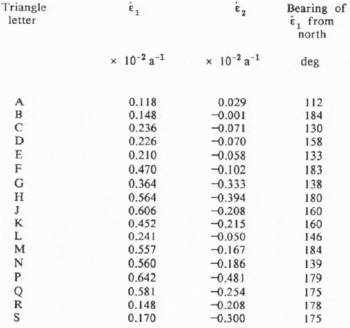
In more detail, the principal strain-rate ε, varied between 0.118 × 10⁻² and 0.642 × 10⁻² a−1. Minima in the value of
Table 1 Horizontal and vertical ice-surface velocities. stakes are located in figure 2


Fig. 5. Horizontal velocity vectors within the trilateration network on Basin 5. Vector length is proportional to horizontal ice-surface velocity.

Fig. 6. Principal strain-rates within the trilateration network on Basin 5. Vectors represent the magnitude and orientation of
Table 2. Experiments (δ values are shown in parts per thousand)
The orientations of principal strain-rate
Mass Balance
Mass inputs to Austfonna are mainly from surface snow accumulation and the formation of superimposed ice. Mass losses also take two principal forms: ablation and melt-water production, combined with the calving of icebergs from the terminal ice cliffs.
Snow lines and accumulation
The behaviour of the snow line on Austfonna during the melt season can be monitored from Landsat MSS imagery (Fig. 7). For the 1978 and 1979 seasons, for example, the snow line in Basin 5 had retreated approximately 20 km from the coast, to an elevation of about 500 m a.s.l. (Fig. 7b). In detail, the situation is more complex because, especially where surface topography is rough, snow accumulation is very variable on a kilometre scale. These local topographic effects are illustrated by the residual snow areas on the summer aerial photograph of the basin margin (Fig. 3).
The accumulation area extends lower than the snow line, however, through the development of a superimposed ice zone (Reference SchyttSchytt, 1964, 1969). The importance of superimposed ice development has also been reported from the 239 m summit of Storøyjøkulen, north-east of Nordaustlandet, where nourishment comes entirely from the refreezing of surface melt water (Reference JonssonJonssen, 1982). On Basin 5, ice was observed directly below winter snow cover in shallow pits as far up the network as station 12 (480 m elevation).
Horizontal ice-surface velocities reach a maximum at stations 14 and 17 on the two lines (Fig. 2a; Table I), and their vertical component progressively approaches zero in the bottom third of the network. Given the tendency for surface-velocity maxima to be associated with the equilibrium line, this evidence suggests that the ablation zone may begin at an elevation of between 330 and 400 m. A 9.8 m ice core collected in 1983 about 25 km to the south-west of Basin 5 at an elevation of 374 m (Isdomen, labelled Is in Figure 1b) supports this inference. The core was analysed for tritium content and the 1963 horizon was identified at a depth of 1 m. The presence of the layer shows that the accumulation of superimposed ice is still taking place at this relatively low elevation, and indicates an average net accumulation of 47 kg m−2 a−1. The equilibrium line cannot be far below this level, and this conclusion supports Schytt's (1964) suggestion that the equilibrium line in north-east Austfonna is at approximately 300 m. As a consequence, the accumulation zone comprises about 65–70% of the surface area of Basin 5.
The rate and spatial variability of accumulation within the basin is not well known. Measurements of the change in snow-surface height around stakes in the trilateral network between May 1986 and May 1987 did not yield useful information on net mass balance. In each of these years, considerable snow accumulation took place during spring blizzards, and the snow-surface height appeared to be dependent on such short-term factors rather than providing a useful record of the annual balance. Soviet analysis of a 204 m core taken at the summit of Austfonna, 30 km distant and 780 m in elevation, has shown an accumulation rate of between 400 and 500 kg m−2 a−1 over approximately the last 400 years (personal communication from V. Zagorodnov). Schytt (1964) recorded a similar value for net accumulation (530 kg m−2 a−1) on the summit of Vestfonna (622 m in elevation). Analysis of total β activity in a Soviet core from Vestfonna gave an accumulation rate of 810 kg m−2 a−1, averaged over a 19 year period (Reference Punning, Martma, Tyugu, Vaykmyae, Pourchet and PinglotPunning and others, 1985). Reference AhlmannAhlmann (1933) had earlier analysed snow stratigraphy in a number of pits on Austfonna and Vestfonna. He suggested a mean net balance of only 60–70 kg m−2 a°1 for the

Fig. 7. The location of snow lines on Austfonna through the melt season. a. Landsat Multispectral Scanner (MSS) band 7 image, showing the position of the snow line on 13 August 1978 (Id. No. 3016112143). The part scene is 130 km wide. b. Locations of the snow line from four Landsat MSS images. Basin 5 is indicated.
accumulation zones, implying a very negative total net balance for the ice caps. However, the observations of both Schytt and Soviet workers on net accumulation show that these earlier values represent a considerable underestimate, probably accounted for by the complexity of the snow stratigraphy on Nordaustlandet.
Assuming an accumulation area of about 440 km2 (65% of the basin), an averaged accumulation rate of between 0.3 and 0.4 m a−1 of ice equivalent would yield a total net gain of 132–176 × 106m3a−1 of ice for that part of Basin 5 above the equilibrium line. A hypsometric curve for the accumulation area shows that approximately 45% of the accumulation basin lies above 600 m. The averaged accumulation rate is therefore weighted towards the values observed at higher elevations.
Balance velocity at the equilibrium line
Balance velocity represents the average velocity required to transport, through a given section, the areally integrated net mass balance above that cross-section. There is an assumption that the ice mass is in a steady state. Negative departures of balance velocity from observed average velocity indicate that net-volume change up-glacier is negative, whereas positive departures signal positive volume changes. Balance velocities (K^) are calculated from the following mass-continuity equation:
where W and H are the transverse width and mean ice thickness at a given section across the drainage basin, Da is basin surface area, and A is the mean accumulation rate above the cross-section. No correction was made for the shape of the cross-section, since the geometry of the transverse profile is relatively simple.
The balance velocity is calculated for a transverse profile running through station 19 which, at an elevation of 330 m, approximates the position of the equilibrium line. The width of this cross-section through Basin 5, the mean ice thickness, and the basin area above it, are obtained from Figure 2. The average accumulation is less well defined at 0.4 ± 0.1 ma−1, and balance velocities are therefore calculated for ±0.1 of the assumed mean value. The result is a balance velocity of 36.6 ± 9 m a−1. Comparison with measured surface velocities at stations 17, 19, and 20 (39, 37, and 36 m a−1; Table I) shows that the observed and calculated values are very comparable. This implies either that Basin 5 is approximately in steady state at the present, or that the spatially averaged values of net accumulation discussed above and used in calculation are considerably in error.
Ablation and iceberg calving
There are no data from the ablation area of Austfonna which can be used to estimate reliably the amount of mass loss through melting at relatively low elevations. In Basin 5, such measurements were particularly problematic due to heavy crevassing (Fig. 3). Only an order-of-magnitude value for the mass lost by iceberg calving can be presented.
Mass is lost at the tide-water terminus of Basin 5 through iceberg calving and by direct melting of the terminal ice cliffs. Both are difficult to quantify. Tabular icebergs of up to 600 m in length have been observed offshore of the east coast of Austfonna during airborne radio echo-sounding flights, and isolated icebergs can also be identified on aerial photographs and Landsat satellite imagery. However, remotely sensed data are not available with sufficient frequency to provide a useful time series of observations. Iceberg-calving rates cannot therefore be reconstructed directly.
However, order-of-magnitude calculations of the combined mass lost at the terminal ice cliffs from the processes of iceberg calving and direct melting may be made. Assume that Basin 5 is in steady state, with a velocity at its terminus of 40 m a−1, and that it averages approximately 130 m in thickness (from RES data) along its 20 km interface with marine waters. For the ice-front position to be maintained, a mass of 100 × 106 m3 a−1 must be lost through the combined action of the two processes. Halving the velocity will clearly halve the rate of mass loss. The assumption that the ice front is stable is difficult to test because, although Landsat images are available for several different years, there is insufficient rock outcrop to fix accurately the ice front of Basin 5. However, the terminal ice cliffs of the basin immediately to the north-east of Basin 5 retreated by almost 500 m between 1976 and 1981 (Reference DowdeswellDowdeswell, 1986b). If the terminus of Basin 5 was also retreating during that period, the mass lost through calving may have been more than double that suggested above.
Subglacial Melt Water
Subglacial debris-rich melt water emerging from Austfonna is important for several reasons. Most significantly, it indicates that at least part of the ice–bed interface is at the pressure melting-point. Secondly, it shows that there is a subglacial source of unlithified material. Thirdly, it represents part of the mass lost by the ice cap each year.
Digital analysis of Landsat imagery has shown plumes of turbid water spreading out from point sources at the tide-water margins of Basin 5, and indeed from much of eastern Austfonna (Fig. 8). These plumes occur at the surface because glacial melt water is less dense than sea-water, except when turbidity is very high. Their inter-pretation as turbid melt-water plumes is confirmed by field measurements of relatively high near-surface suspended sediment concentration offshore of eastern Austfonna (personal communication from A. Solheim). Their origin is subglacial, because there are no sources of supraglacial sediment on the east side of Austfonna, and their debris load must therefore be derived from the glacier bed. Their emergence at discrete points indicates that water flow is in subglacial conduits. Analysis of several Landsat images shows that the position of these suspended-sediment plumes is relatively stable over time. Some are associated with troughs within the bed of Austfonna, and therefore with thicker ice, but this link is not a general one (Fig. 8b).
Several glaciological implications can be drawn from the presence of these major subglacial drainage channels at the margins of Basin 5 and the other drainage basins in northeast Austfonna. First, they provide direct evidence for the presence of water and therefore of melting at the base of Austfonna. Significantly, this melting extends to the margins of the ice cap at least in some terminal areas (Fig. 8). The thermal structure of Austfonna is complex, however, and forms the subject of a separate analysis (paper in preparation by D.J. Drewry and others). Secondly, the presence of suspended sediments within the melt water not only allows their identification on Landsat imagery but also indicates that there is a subglacial source of unlithified material. Unfortunately, there is no direct evidence to suggest whether this debris is derived from a till substrate of significant thickness and lateral extent, or if unlithified material is simply supplied by continuing glacial erosion of exposed bedrock.
Nature of the Substrate Underlying Basin 5
Recent evidence concerning the presence of unlithified, deformable sediments underlying some ice masses has emphasized the need for more precise specification of the basal boundary condition in modelling studies (e.g. Reference Blankenship, Bentley, Rooney and AlleyBlankenship and others, 1986). The mechanics of any subglacial sediment, as well as the thermal characteristics of the ice–bed interface, are therefore of considerable significance (Reference Boulton and HindmarshBoulton and Hindmarsh, 1987; Reference ClarkeClarke, 1987).
Indirect evidence from airborne radio echo-sounding returns is equivocal. In Antarctica, it is possible to infer the presence of water beneath certain outlet glaciers from radio echo-strength measurements (Reference NealNeal, 1976; Reference McIntyreMclntyre, 1985). On Nordaustlandet, however, the ice is closer to its melting point, and thermally more complex. Calculation and interpretation of bed-reflection coefficients is therefore problematic due to variations in absorption and scattering losses (personal communication from J.L. Bamber).
Marine geological surveys immediately offshore of east Austfonna show that the substrate recently exposed by ice-

Fig. 8. a. Plumes of subglacial melt water emerging from the tide-water terminus of Leighbreen, north-east Austfonna, imaged in a Landsat MSS band 5 scene acquired on 16 August 1979 (Id. No. 2338001093). The part scene is 30 km wide. b. Location of major outlets of subglacial melt water along the east coast of Austfonna, identified in the 16 August 1979 Landsat MSS scene. Large arrows represent the most important suspended-sediment plumes, in terms of their relatively large areal extent and higher sediment concentration.
mass retreat is composed of deformable sediment rather than bedrock (Reference SolheimSolheim and Pfirman, 1985; Reference Solheim and PfirmanSolheim, 1986). Side-scan sonar and shallow seismic reflection investigations provide morphological and stratigraphical evidence for the presence of soft sediments which were overlain by the surge-type drainage basin, Brasvellbreen, after its rapid advance between 1936 and 1938 (Reference SchyttSchytt, 1969). Sediments of similar surface morphology also lie immediately beyond the basin associated with Isdomen (Fig. 1b), which is inferred to have surged recently on both marine geological and glaciological grounds (Reference DowdeswellDowdeswell, 1986a; Reference SolheimSolheim, 1986). Advances of any other Austfonna tide-water outlets will be over a deformable substrate derived from glacimarine sedimentation. Similarly, over 28% of Austfonna rests on a bed that is below present sea-level, including about 30% of Basin 5 (Fig. 8). It is probable that marine sediments have accumulated here during past periods when Austfonna was smaller than it is today. Thus, the likelihood is that at least one-third of Basin 5 is underlain by deformable sediments, with the nature of the substrate beneath the remainder being less certain.
Conclusions
A number of glaciological field measurements have been described, which are fundamental prerequisites to modelling studies of Austfonna, the largest ice cap on Nordaustlandet, Svalbard. The ice cap is a very suitable one for such modelling studies because of the relative simplicity of its basal and surface topography, together with the knowledge that basins within it behave in several distinctive ways (including surging). The results from deep ice cores through Austfonna will also provide palaeoclimatic forcing for the modelling of ice-cap dynamics over time, and marine geological evidence will assist in constraining palaeo-ice-front positions.
The boundary conditions discussed here have dealt with both the upper and lower ice-cap interfaces. One drainage area, Basin 5, has been considered in detail, but some measurements can be generalized over much larger areas of Austfonna. The ice-surface and bed morphology of Basin 5 is mapped in detail. The first measurements of ice-surface velocities and strain-rates on Austfonna are presented, showing a maximum observed velocity at the equilibrium line of 47 m a−1. Mass-balance data for the ice cap are discussed and a comparison of balance with observed velocity at the equilibrium line suggests that the basin is approximately in balance. A first approximation for the rate of iceberg calving is also given. Subglacial melt water is observed issuing from the tide-water terminus of north-east Austfonna, implying that at least part of the outer margin of the ice mass is at the melting point. Finally, some comments are made on the nature of the substrate. It is likely that, around the perimeter of the ice cap at least, parts of the ice mass are underlain by unlithified sediments. Some inferences on the thermal structure of Austfonna are also made here, but direct field observations and calculations of the temperature distribution through the ice cap are considered in detail in a separate paper (paper in preparation by D.J. Drewry and others). Together, these data provide a relatively comprehensive set of boundary conditions which allow us to model mathematically both the present dynamics of Austfonna (paper in preparation by L.G. Watts and others) and then to step such a model both backward and forward through time.
Acknowledgements
This research was funded by U.K. Natural Environment Research Council grant GR3/4663. The field programme was conducted when both authors were at the Scott Polar Research Institute, University of Cambridge. We thank T.R. Duggleby, M.R. Gorman, R.K. Headland, and L.G. Watts for assistance with velocity measurements and data reduction, and Sysselmannen pȧ Svalbard for permission to work in Nordaust-Svalbard Naturreservat. Dr S. Helle kindly gave permission to reproduce an aerial photograph from the Norsk Polarinstitutt collection. E.K. Dowdeswell assisted in the production of this paper.


