


1. Introduction
The financialization trend, including household debt accumulation, has been a major characterization of the global economy in recent decades. However, this trend has not been without major cycles and crises such as the global financial crisis [Mian and Sufi (Reference Mian and Sufi2014)]. The financialization trend and the corresponding volatilities have also led to higher levels of research activity on the mechanisms and consequences of financial developments, as well as the finance-growth nexus and associated boom-bust cycles [Tornell and Westermann (Reference Tornell and Westermann2005), Schularick and Taylor (Reference Schularick and Taylor2012), Mian et al. (Reference Mian, Sufi and Verner2017)]. When the relevant studies are examined, it is found that they generally focus on the implications of finance on the aggregate output, with relatively scarce literature on the disaggregated or sector-level effects [Varela (Reference Varela2017)]. The present paper aims to fill this research gap by documenting the short-run and medium-run effects of household and firm credits on the dynamics of manufacturing (a proxy for the tradable sector) and services (a proxy for the non-tradable sector) sectors for a large sample of 41 advanced and developing countries.
In order to identify the time-varying effects of the changes in the household and firm credits to GDP ratios on the sector-level output dynamics, we follow the empirical strategy of Mian et al. (Reference Mian, Sufi and Verner2017) in terms of fixed-effects panel data estimations. We first replicate the results of Mian et al. (Reference Mian, Sufi and Verner2017) and show that an increase in the household credit to GDP ratio creates short-run positive effects and medium-run negative effects on the aggregate output growth. As a main additional result to Mian et al. (Reference Mian, Sufi and Verner2017), the analysis indicates that this boom-bust cycle is mainly observed in the case of developing countries, with no short-run positive effects of household credits for the advanced countries. Moreover, the effect sizes are quite large in both advanced and developing countries. For example, a one standard deviation increase in the household debt to GDP ratio over the last three years (7.1 percentage points for advanced countries and 5.2 percentage points for developing countries) is associated with a 2.20 percentage point decline in GDP over the next three years for advanced countries and a 1.97 percentage point decline for developing countries. As another main additional result, the present paper shows that the boom-bust cycles (i.e. short-run positive effects and medium-run negative effects) arising from the household credit are mainly observed in the services sector, with no similar cycles in the manufacturing sector. In addition, the panel data regressions indicate the medium-run negative effects of the household credits are larger in the case of the manufacturing sector. For instance, a one standard deviation increase in the household debt to GDP ratio over the last three years (6.4 percentage points for the full sample of advanced and developing countries) is associated with a 4.49 percentage point decline in the manufacturing output over the next three years and a 1.23 percentage point decline in the services sector output. So, the manufacturing sector is found to be more sensitive to credit developments. As a robustness analysis, we also implement seemingly unrelated regression (SUR) estimations to control for possible contemporaneous cross-equation error correlations among manufacturing and services sectors. The findings of the SUR analysis also confirm the results from the panel data regressions. Moreover, in order to display the dynamic effects of credit changes on the sector-level output, panel VAR estimations are conducted following the approach of Love and Zicchino (Reference Love and Zicchino2006). These findings also confirm the general findings in the paper. Overall, the present paper expands the existing literature on the finance-growth nexus in terms of differences across advanced-developing countries and manufacturing-services sectors.
The credit-driven business cycles in advanced and developing countries are acknowledged empirically and theoretically in the literature, and the second section discusses them in detail. The empirical results obtained in the present paper have important implications for the relevant literature and the theoretical models as it shows that these cycles differ to a large extent across countries and sectors. There can be different factors behind these findings. For example, relatively low levels of financial development and weak contract enforceability can lead to stronger boom-bust cycles in developing countries [Ranciere et al. (Reference Ranciere, Tornell and Westermann2008)]. Similarly, the presence of foreign currency borrowing and pecuniary externalities can increase the credit sensitivity of output in these countries [Bianchi (Reference Bianchi2011)]. Regarding the differential credit-driven cycles across manufacturing and services sectors, similar arguments can apply in the sense that financial constraints can be more binding in the services sector [Tornell and Westermann (Reference Tornell and Westermann2005)], thereby leading to credit-driven boom-bust cycles in this sector. As another possible mechanism, credit booms (especially household credits) can lead to the appreciation of the domestic currency [Bahadir and Gumus (Reference Bahadir and Gumus2016)], with negative effects of appreciation on the growth of the manufacturing sector [Rodrik (Reference Rodrik2008)]. Hence, the negative medium-term impacts of household credit can be stronger in the manufacturing sector than in the services sector. There can also be other factors that can create differential sector-level sensitivities such as different labor intensities, input-output linkages, product differentiation, returns to scale, and external finance dependence levels. Overall, the heterogenous credit-driven business cycles across countries and sectors can be justified using different theoretical mechanisms, and the present paper establishes the relevant empirical regularities strongly using a comprehensive dataset.
The rest of the paper is structured as follows. The next section provides a critical literature review and discusses the contribution and differences of the present paper. Then, the third section provides details of the methodological approach utilized, while the fourth section presents the data and summary statistics. The fifth section gives the results of the panel data regressions, while the sixth section provides additional robustness analyses. Finally, the last section concludes the paper. Additional regression results and panel VAR findings are presented in the appendices.
2. Literature review
There is a growing literature that examines the relationship between financial markets and the real economy. Earlier studies such as King and Levine (Reference King and Levine1993) and Levine (Reference Levine2005) argue that financial sector development positively affects economic growth. However, more recent studies, especially after the global financial crisis, document the possible negative consequences of the financial markets [Jorda et al. (Reference Jorda, Schularick and Taylor2013)]. For example, Schularick and Taylor (Reference Schularick and Taylor2012, p.1029) examine data for 14 advanced countries covering the 1870-2008 period and show that “Credit growth is a powerful predictor of financial crises.” Various papers try to provide some theoretical mechanisms for these finance-growth dynamics [Hall (Reference Hall2011)]. Eggertsson and Krugman (Reference Eggertsson and Krugman2012) show that if the high-debt agents are credit-constrained, then there can be strong debt deflation and liquidity trap dynamics in the economy with major effects on economic output. Guerrieri and Lorenzoni (Reference Guerrieri and Lorenzoni2017) study a mechanism where the borrowing capacity of the consumers is tightened permanently. In this case, the constrained consumers would be forced to deleverage, and the unconstrained consumers would increase their precautionary savings. Both mechanisms would lead to a large decline in economic output, even without any nominal stickiness in the economy. Different papers provide alternative mechanisms such as contract enforceability and bailout guarantees in Schneider and Tornell (Reference Schneider and Tornell2004), limited commitment and pecuniary externalities in Lorenzoni (Reference Lorenzoni2008), externalities in the foreign currency borrowing of small open economies in Bianchi (Reference Bianchi2011), and demand externalities and liquidity traps in Korinek and Simsek (Reference Korinek and Simsek2016). Overall, these papers offer different mechanisms on how various financial market imperfections and conditions lead to excessive borrowing and leverage that would produce costly economic crises in the following periods.
One common feature of the above studies, such as Schularick and Taylor (Reference Schularick and Taylor2012) and Jorda et al. (Reference Jorda, Schularick and Taylor2013), is that they generally look at the relationship between the total private sector credit and the total economic output. A new strand of the relevant literature also makes a distinction between the credit types and their effects on economic output [Mian and Sufi (Reference Mian and Sufi2011), (Reference Mian and Sufi2014), (Reference Mian and Sufi2018)]. For example, Mian et al. (Reference Mian, Sufi and Verner2017) examine the case of 30 advanced and developing countries covering the period of 1960–2012. Their results indicate that a rise in the household debt in the last three years is associated with a moderate increase in the economic output in the short run, while it leads to large negative growth effects in the medium and long run. Similar effects are also found in the case of consumption and unemployment. Hence, this paper shows that household debt is quite influential in affecting the business cycles in both advanced and developing countries. In contrast, Mian et al. (Reference Mian, Sufi and Verner2017) find that firm debt does not produce sizeable growth and business cycle effects. Lombardi et al. (Reference Lombardi, Mohanty and Shim2017) also find similar results with a larger sample of 54 countries covering the more recent periods of 1990–2015. Namely, a rise in the household debt-GDP ratio leads to a higher growth rate in the short run and a lower growth rate in the long run.
While there is a growing number of studies examining the effects of “different credit types,” the literature regarding the credit market effects on “different output types” is relatively limited. One underlying reason is that the majority of the existing theoretical and empirical studies do not have explicit mechanisms which would necessitate separate effects for the different sectors of the economy. As an important early study on the topic, Tornell and Westermann (Reference Tornell and Westermann2002) examine the dynamics and characteristics of the boom-bust cycles in middle-income countries. Their results indicate that the real credit gap and credit/GDP ratio increase before the crises and then decline afterwards significantly. In the process, the real GDP gap also displays a boom-bust cycle. These results are consistent with the other studies in the literature such as Schularick and Taylor (Reference Schularick and Taylor2012) and Jorda et al. (Reference Jorda, Schularick and Taylor2013). One important contribution of Tornell and Westermann (Reference Tornell and Westermann2002), Tornell et al. (Reference Tornell, Westermann and Martinez2003), and Tornell and Westermann (Reference Tornell and Westermann2005) is that the authors also examine the composition of output and the real exchange rates around the crises. They find that the non-tradable output as a ratio to the tradable output and the real exchange rate also displays boom-bust cycles. As a possible mechanism explaining the asymmetric response of the sector-level output to the credit cycle, the authors note that the firms in the non-tradable sectors face tighter financial constraints. Under such differential financial constraints, it becomes possible for the credit cycles to produce asymmetric effects on the output dynamics of different sectors. In a theoretical model, Schneider and Tornell (Reference Schneider and Tornell2004) offer fundamental factors (such as asymmetric financing conditions in the N and T sectors, along with implicit bailout guarantees) that can account for the asymmetric dynamics of the N and T sectors around the financial crises.
There are only a few papers that consider the possibility of the aforementioned asymmetric sectoral dynamics. For example, Varela (Reference Varela2017) examines the asymmetric response of the tradable and non-tradable sector outputs to the credit market conditions in a sample of 35 advanced and developing countries covering the 1992−2015 period. The results indicate that non-tradable output is positively responsive to credit growth, while tradable output is not responsive. In addition, these results are mostly observed in emerging countries. In a very recent study, Mian et al. (Reference Mian, Sufi and Verner2020) examine how credit supply expansion affects the real economy. The authors conduct a detailed analysis in the case of the US and find that the credit supply expansions lead to rises in the non-tradable output and employment. In contrast, the effects on tradable output and employment are found to be limited. The authors also conduct a short analysis of the panel sample of 56 countries. The panel data estimations indicate that credit growth, especially household debt growth, is positively associated with the N/T output and employment ratios, as well as the real exchange rate. There are also papers that try to model these dynamics of sectoral asymmetries within real business cycle models like Bahadir and Gumus (Reference Bahadir and Gumus2016) and Kehoe et al. (Reference Kehoe, Lopez, Midrigan and Pastorino2020).
The present study extends the relevant literature in terms of various dimensions. In the case of Varela (Reference Varela2017) and Mian et al. (Reference Mian, Sufi and Verner2020), the authors implement panel data regressions where the relationship between credit and sectoral output is estimated for one specific period. It is possible that this relationship is more dynamic. Hence, it becomes a useful extension to estimate the credit-sectoral output relationship over different time horizons. In that context, the present study follows Mian et al. (Reference Mian, Sufi and Verner2017) and runs regressions between credit types and sectoral output for various time horizons. In this way, the credit-output relationship is mapped in a broader temporal spectrum. As another extension to the relevant literature, the present study collects data from a large set of advanced and developing countries and identifies the differences between these two country groups. This is an important research area, as the financial conditions and cycles might matter more for some countries than others. For example, the size of household credit is much smaller in developing countries relative to advanced countries. Then, it is possible that the business cycle and sectoral output impact of the household credit can differ across developing and advanced countries. As another point, studies such as Tornell and Westermann (Reference Tornell and Westermann2005) and Mian et al. (Reference Mian, Sufi and Verner2020), except for Varela (Reference Varela2017), mainly examine the effect of credit on an indicator for the ratio of non-tradable (N) and tradable (T) sectors. However, the separate dynamics of the N and T sectors also become informative in understanding the sectoral effects. This is especially true in the case of the leading T sector, that is, manufacturing, and the leading N-sector, that is, services. Understanding the relationship can be useful for the literature on the structural transformation of the economies. For example, the relevant studies discuss the role of incomes, sectoral productivities, and relative prices in driving the structural transformation in the US and other countries [Duarte and Restuccia (Reference Duarte and Restuccia2010), Herrendorf et al. (Reference Herrendorf, Rogerson and Valentinyi2013)]. Credit dynamics, like the changing shares of the household and corporate credits, can be an important factor in explaining the structural transformation. Hence, it is valuable to see how credit developments affect the leading sectors in an economy. Overall, the present paper aims to expand the existing literature on several dimensions as discussed above.
3. Methodology
The studies in the literature use various panel data methods to examine the cross-country relationship between the credit markets and real economic variables. For example, Varela (Reference Varela2017) uses pooled mean group estimator methods, which take the individual dynamics of each country into account. In the case of Mian et al. (Reference Mian, Sufi and Verner2017), the authors use an instrumental variable fixed-effects method to control for the possible endogeneity of the regressors. They also cluster errors on country and year to control for both within-country and contemporaneous cross-country correlations. In the case of Mian et al. (Reference Mian, Sufi and Verner2020), the authors use the fixed-effects model with robust standard errors and cross-sectional dependence [Driscoll and Kraay (Reference Driscoll and Kraay1998)]. As the research design of the present paper follows the regression equations of Mian et al. (Reference Mian, Sufi and Verner2017), the present study also implements the fixed-effects model as the baseline method. The main regression equation is given as follows:
 \begin{equation} \triangle _{3}y_{it+k}=\alpha _{i}+\beta _{HH}\triangle _{3}Credit^{HH}_{it-1}+\beta _{F}\triangle _{3}Credit^{F}_{it-1}+X^{\prime}_{it-1}\Gamma +u_{it+k} \end{equation}
In the above equation, k takes values in the range of −1, 0, 1, $\ldots$
, 5. On the right-hand side, the credit variables are the debt stocks of households and firms as a ratio to their respective income levels. In the case the total credit to the private sector is used, it is estimated as a ratio to the GDP of the country.
$\ldots$
, 5. On the right-hand side, the credit variables are the debt stocks of households and firms as a ratio to their respective income levels. In the case the total credit to the private sector is used, it is estimated as a ratio to the GDP of the country. $X^{\prime}_{it-1}$
is the set of control variables.
$X^{\prime}_{it-1}$
is the set of control variables.
In order to see how the above specification displays the relevant information on the credit-output relationship in a temporal way, examining the equation details in some cases would be useful. For example, in the case of k = −1, the dependent variable becomes $\triangle _{3}y_{it-1}$
, and the main independent variables become
$\triangle _{3}y_{it-1}$
, and the main independent variables become $\triangle _{3}Credit^{HH}_{it-1}$
and
$\triangle _{3}Credit^{HH}_{it-1}$
and $\triangle _{3}Credit^{F}_{it-1}$
. So, output and credit variables become contemporaneous (i.e. the relevant periods fully overlap) and the regression estimates the impact of 3-year credit differences on the 3-year output difference. As k increases, the periods of credit and output get separated at a higher rate. For example, in the case of k = 4, the dependent variable becomes
$\triangle _{3}Credit^{F}_{it-1}$
. So, output and credit variables become contemporaneous (i.e. the relevant periods fully overlap) and the regression estimates the impact of 3-year credit differences on the 3-year output difference. As k increases, the periods of credit and output get separated at a higher rate. For example, in the case of k = 4, the dependent variable becomes $\triangle _{3}y_{it+4}$
, and the main independent variables are still
$\triangle _{3}y_{it+4}$
, and the main independent variables are still $\triangle _{3}Credit^{HH}_{it-1}$
and
$\triangle _{3}Credit^{HH}_{it-1}$
and $\triangle _{3}Credit^{F}_{it-1}$
. In this case, the regression estimates the impact of the credit change from four years ago to the last year on the output change from the following year to the four years in future. Overall, by running the equation (1) for seven different temporal relationships (i.e. k = −1, 0, 1,
$\triangle _{3}Credit^{F}_{it-1}$
. In this case, the regression estimates the impact of the credit change from four years ago to the last year on the output change from the following year to the four years in future. Overall, by running the equation (1) for seven different temporal relationships (i.e. k = −1, 0, 1, $\ldots$
, 5), one can get a detailed map of the credit-output relationship. It needs to be noted that as the time span requirements change across these different specifications, the number of countries and observations would also vary due to the unbalanced nature of the dataset. As another important feature, equation (1) examines the 3-year differences in the output and credit variables. In this way, the high-frequency and volatile nature of the yearly changes is not utilized in the regression estimations. These features of equation (1) are important differences from other studies like Tornell and Westermann (Reference Tornell and Westermann2005) and Varela (Reference Varela2017), which use yearly changes and examine only contemporaneous or one-lag relationships. In line with the cases of Mian et al. (Reference Mian, Sufi and Verner2017) and (Reference Mian, Sufi and Verner2020), the errors are clustered on year and country. As the regression variables move in an overlapping way, it is natural to have within-country correlations. Besides, the common global shocks can create correlations among the countries. Hence, clustering the errors on country and year is expected to control for such cases. As a robustness analysis, the SUR estimations are also implemented to control for possible contemporaneous cross-equation error correlations among manufacturing and services sectors. Moreover, various robustness estimations are conducted such as the inclusion of control variables, crisis dummies and their interactions with credit variables, and distributed lags, and the use of different datasets and definitions for the services sector to exclude the financial sector from the analysis.
$\ldots$
, 5), one can get a detailed map of the credit-output relationship. It needs to be noted that as the time span requirements change across these different specifications, the number of countries and observations would also vary due to the unbalanced nature of the dataset. As another important feature, equation (1) examines the 3-year differences in the output and credit variables. In this way, the high-frequency and volatile nature of the yearly changes is not utilized in the regression estimations. These features of equation (1) are important differences from other studies like Tornell and Westermann (Reference Tornell and Westermann2005) and Varela (Reference Varela2017), which use yearly changes and examine only contemporaneous or one-lag relationships. In line with the cases of Mian et al. (Reference Mian, Sufi and Verner2017) and (Reference Mian, Sufi and Verner2020), the errors are clustered on year and country. As the regression variables move in an overlapping way, it is natural to have within-country correlations. Besides, the common global shocks can create correlations among the countries. Hence, clustering the errors on country and year is expected to control for such cases. As a robustness analysis, the SUR estimations are also implemented to control for possible contemporaneous cross-equation error correlations among manufacturing and services sectors. Moreover, various robustness estimations are conducted such as the inclusion of control variables, crisis dummies and their interactions with credit variables, and distributed lags, and the use of different datasets and definitions for the services sector to exclude the financial sector from the analysis.
4. Data and summary statistics
The relevant data for the empirical analysis are collected from two public sources. The macroeconomic variables, including the real growth rates of the GDP, manufacturing sector output (as a proxy for the tradable sector), and services sector output (as a proxy for the non-tradable sector), are obtained from the World Development Indicators database of the World Bank (2021). The sample includes the 1960–2019 period. However, there are many missing observations, especially in the early decades, thereby leading to an unbalanced panel. Then, the credit data (i.e. total credit to the private sector, as well its decomposition in terms of credit to households and firms) are obtained from the Bank for International Settlements (BIS, 2022). These data are collected for 41 advanced and developing countries. The sample includes the following advanced countries: Australia, Austria, Belgium, Canada, Denmark, Finland, France, Germany, Greece, Ireland, Israel, Italy, Japan, Netherlands, New Zealand, Norway, Portugal, Spain, Sweden, Switzerland, the United Kingdom, and the United States. In addition, the sample includes the following developing countries: Argentina, Brazil, Chile, Colombia, Czechia, Hungary, India, Indonesia, Korea, Malaysia, Mexico, Poland, Russia, Saudi Arabia, Singapore, South Africa, Thailand, and Turkey. It is seen that the sample of developing countries consists of major emerging economies with sufficiently developed credit markets, at least during recent decades. These two data sources are combined to obtain the final sample. The summary statistics of this sample are presented in Table 1 below.
Table 1. Summary statistics
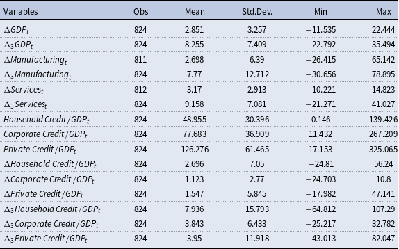
Table 1 shows that the number of observations in the sample is larger than 800.Footnote 1 The average real GDP growth rate is estimated at 2.85%, with a standard deviation of 3.26%. In the case of medium-run effects, the study looks at the three-period differences of the relevant variables. It is found that this medium-run variable has an average of 8.26%, with a standard deviation of 7.41%. In the case of the manufacturing sector, the one-period growth rate is estimated at 2.70%, while the three-period growth rate is estimated at 7.77%. Then, in the case of the services sector, the one-period growth rate is estimated at 3.17%, while the three-period growth rate is estimated at 9.16%. So, the sample has the property that the growth of the services is higher than the manufacturing growth rate, implying a rising share of services in the economy. Regarding the credit variables, the average private sector credit is estimated at 126.28% as a ratio to GDP, with a standard deviation of 61.47%. When the decomposition of private credits is examined, it is seen that household credits have an average of 48.96%, while corporate/firm credits have a mean of 77.68%.
In order to provide a relevant example, Figures 1 and 2 present the dynamics of credits and output in the United States around the global financial crisis of 2007–2009. It is seen that in the early 2000s, the credit growth rates for the households and corporates were at similar rates, whereas a household credit boom followed in the mid-2000s where the three-period change in the household credit to GDP ratio reached close to 15%, while the three-period change in the corporate credit to GDP ratio was around 0%. Then, after the global financial crisis, a bust in household credits was observed, while corporate credits displayed some recovery. So, household credit was much more volatile in the US around the financial crisis. Figure 2 shows that in the same period, the manufacturing sector was also more volatile than the services sector. The manufacturing sector experienced a boom before the household credit rise and experienced a sharp decline with the crisis. Hence, the present paper tries to document if there exists a link between the cycles of different credit types and the sector-level output dynamics in the sample of advanced and developing countries. As the previous sections displayed, a medium-run negative relationship between household credits and aggregate output is firmly established by Mian et al. (Reference Mian, Sufi and Verner2017). The present paper expands this relationship to the domain sector-level output.

Figure 1. Three-Period credit/GDP difference in the United States (%).

Figure 2. Three-Period real growth of sector outputs in the United States (%).
The relationship between the sector-level outputs and different credit types is not examined in detail in the literature. The previous sections showed that there is a number of studies looking at various dimensions of this relationship. The present paper aims to contribute to the relevant literature by providing a comprehensive account of the possible short-run and medium-run relationships between different credit types and sector-level output dynamics. Before moving to the empirical analysis, Figures 3 and 4 provide a graphical representation of these bivariate relationships. The three-period differences of the relevant variables are used in the graphs to be consistent with the regression equations presented in the methodology section. Figure 3 shows the scatter plots of sector-level outputs relative to the household credit to GDP ratio. A negative relationship is found for the growth rates of both the manufacturing and service sectors. However, it is also seen that the slope of the fit line is larger in absolute value for the manufacturing sector. Hence, Figure 3 provides some initial insights that manufacturing sector growth can be more sensitive to the household credit cycles. Figure 4 shows that this sensitivity with respect to corporate credits is smaller and does not differ across sectors.
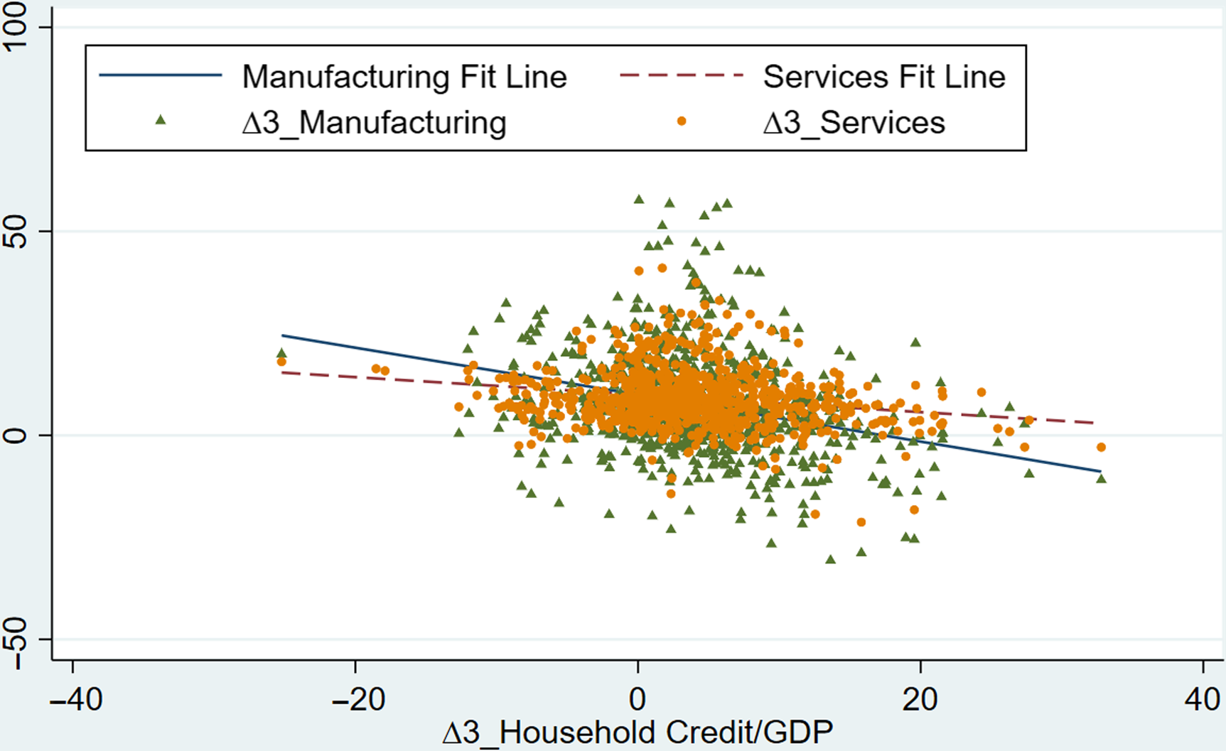
Figure 3. Scatter plots between three-Period differences of household credit and outputs.
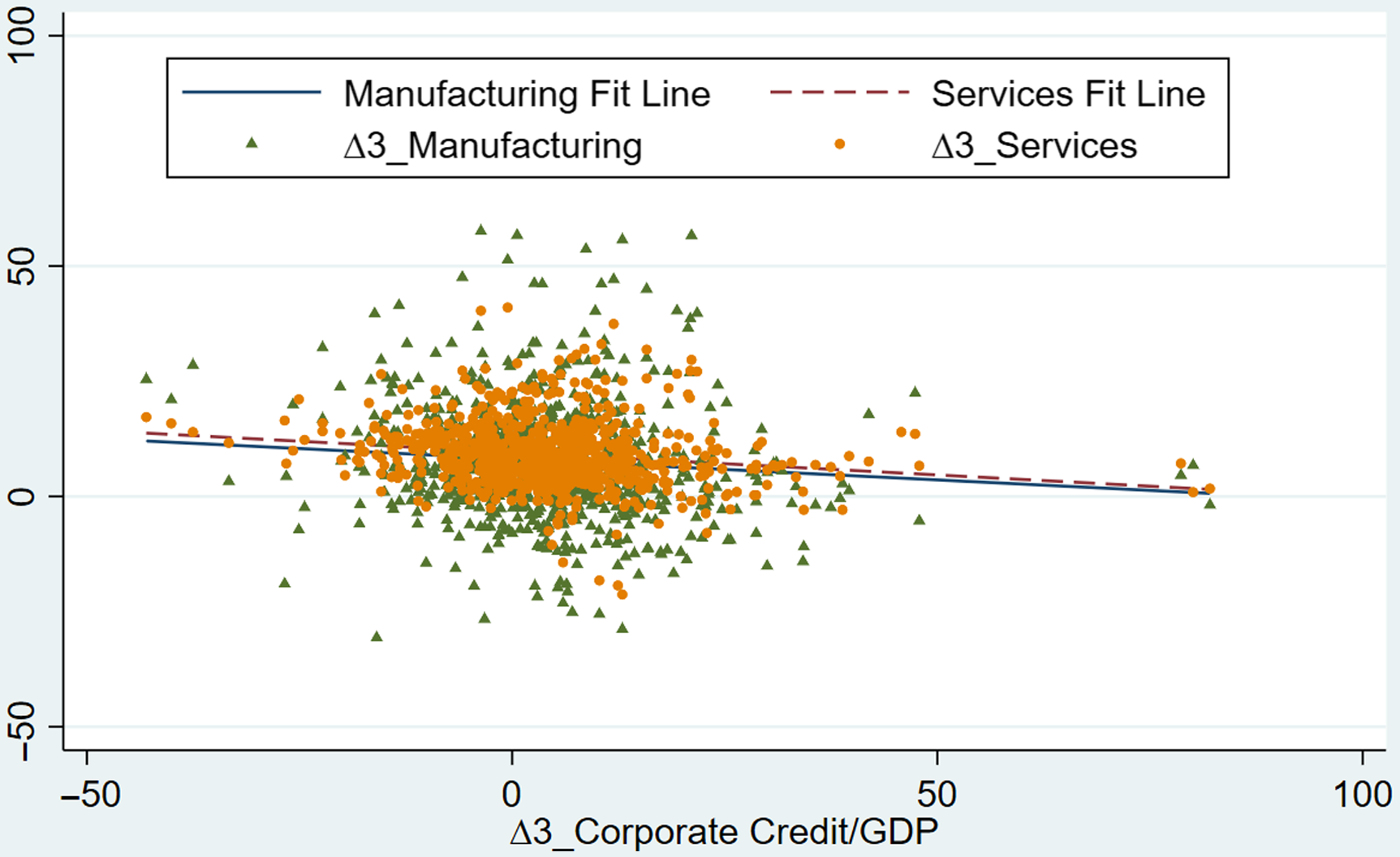
Figure 4. Scatter plots between three-Period differences of corporate credit and outputs.
This section has shown that in the present sample of 41 advanced and developing countries, there is a medium-run negative association between credit movements, especially from household credits, and sector-level output dynamics, especially in the manufacturing sector. The following section provides regression evidence on these relationships following the methodological approach of Mian et al. (Reference Mian, Sufi and Verner2017).
5. Panel regression results
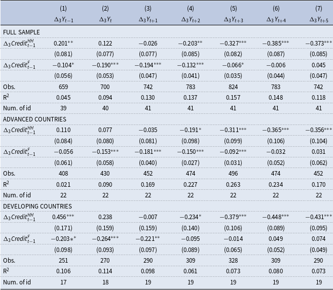
The methodology section reviewed some of the empirical strategies utilized in the relevant literature, such as the pooled mean group estimator in Varela (Reference Varela2017) and the instrumental variable fixed-effects method in Mian et al. (Reference Mian, Sufi and Verner2017). The latter approach also clusters errors on country and year to control for both within-country and contemporaneous cross-country correlations. The present paper follows the latter study as it aims to document the credit growth nexus in both short and medium runs. Then, the regression model presented in equation (1) becomes the benchmark regression. In this context, Table 2 presents the fixed-effects regression of the real output growth on household and firm credits.Footnote 2 In a way, this table replicates the results of Mian et al. (Reference Mian, Sufi and Verner2017) in their Table II. For example, in the first panel and first column of Table 2, the regression coefficient of the household credit is found to be 0.201, while Mian et al. (Reference Mian, Sufi and Verner2017) find this coefficient to be 0.176. In both cases, the regression coefficients are statistically significant at the 5% level. Similarly in the first panel and fifth column of Table 2, the coefficient of the household credit is estimated as −0.327, while Mian et al. (Reference Mian, Sufi and Verner2017) find this coefficient to be -0.337. In these cases, the regression coefficients are statistically significant at the 1% level. Hence, the results of Table 2 in the present paper and Table II of Mian et al. (Reference Mian, Sufi and Verner2017) are very close to each other, with differences arising mainly from the sample coverage where Mian et al. (Reference Mian, Sufi and Verner2017) have 30 countries and the present paper has 41 countries. The regression coefficient of −0.327 implies that a one standard deviation increase in change in the household debt to GDP ratio in the last three years (i.e. 6.4% as shown in Table 1) would correspond to a 2.1 percentage point lower growth in the following three years. Given that the average growth rate in three years is estimated as 8.3%, these numbers imply that the medium-run negative effects of household credit on economic growth are economically large as well.
Table 2. Fixed-effects regression of the real output growth on household and firm credit
The table shows the results of the fixed-effects panel regression ${\Delta }_3Y_{it+k}={\alpha }_i+{\beta }_{HH}{\Delta }_3{Credit}^{HH}_{it-1}+{\beta }_F{\Delta }_3{Credit}^F_{it-1}+u_{it+k}$
, where k = −1, 0, … 5. The dependent variable
${\Delta }_3Y_{it+k}={\alpha }_i+{\beta }_{HH}{\Delta }_3{Credit}^{HH}_{it-1}+{\beta }_F{\Delta }_3{Credit}^F_{it-1}+u_{it+k}$
, where k = −1, 0, … 5. The dependent variable ${\Delta }_3Y_{it+k}$
is the three-year logarithmic change in the reel GDP level in period t + k. The independent variables
${\Delta }_3Y_{it+k}$
is the three-year logarithmic change in the reel GDP level in period t + k. The independent variables ${\Delta }_3{Credit}^{HH}_{it-1}$
and
${\Delta }_3{Credit}^{HH}_{it-1}$
and ${\Delta }_3{Credit}^F_{it-1}$
are the three-year changes in the household and non-financial firm credit to GDP ratio in period t−1, respectively. Standard errors are clustered across countries and years and given in parentheses, with ***
p
${\Delta }_3{Credit}^F_{it-1}$
are the three-year changes in the household and non-financial firm credit to GDP ratio in period t−1, respectively. Standard errors are clustered across countries and years and given in parentheses, with ***
p $\mathrm{\lt }$
0.01, **
p
$\mathrm{\lt }$
0.01, **
p $\mathrm{\lt }$
0.05, *
p
$\mathrm{\lt }$
0.05, *
p $\mathrm{\lt }$
0.1.
$\mathrm{\lt }$
0.1.
In addition to replicating the results of Mian et al. (Reference Mian, Sufi and Verner2017), the above table also provides the analysis of the same effects for advanced and developing countries separately, partly thanks to the larger cross-sectional size of 41 countries. The middle and lower panels of Table 2 show that the negative medium-run effects of household credit on the real output growth are stronger in developing countries compared to advanced countries. In addition, the short-run positive effects of household credits on economic growth exist only in developing countries, with no similar effects in advanced countries. Hence, Table 2 expands the findings on the growth-credit nexus across countries.
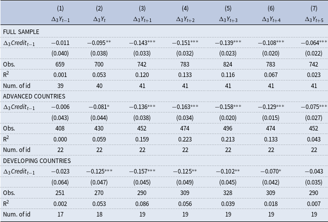
After repeating the analysis of Mian et al. (Reference Mian, Sufi and Verner2017), Tables 3 and 4 present the main regression results of the present paper by looking at the effects of the dynamics of different credit types on the short-run and medium-run growth rates of the manufacturing and services sectors, respectively. When the full sample results in the upper panel of Table 3 are examined, it is found that there are no statistically significant effects of household credits in the short-run, whereas there are negative and statistically significant medium-run effects on manufacturing growth. For example, model (5) of the upper panel in Table 3 finds that the regression coefficient of the change in household credit to GDP ratio is estimated at −0.701 with a 1% statistical significance, while the regression coefficient of the change in the firm credit to GDP ratio is estimated at 0.004 with no statistical significance. The regression coefficient of −0.701 for the household credit implies that a one standard deviation increase in change in the household debt to GDP ratio in the last three years (i.e. 6.4% as shown in Table 1) would correspond to a 4.49 percentage point lower growth of the manufacturing sector in the following three years. Given that the average growth rate in the manufacturing sector in three years is estimated as 7.77%, these numbers imply that the medium-run negative effects of household credit on manufacturing growth are economically large as well. When the differences across advanced and developing countries are examined in the middle and lower panels of Table 3, no major differences are spotted in the effects of the household credits.
Table 3. Fixed-effects regression of the real manufacturing growth on household and firm credit
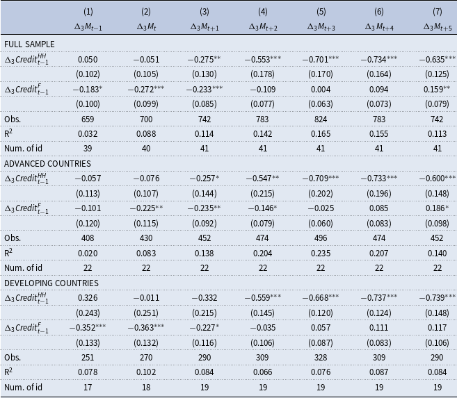
The table shows the results of the fixed-effects panel regression ${\Delta }_3M_{it+k}={\alpha }_i+{\beta }_{HH}{\Delta }_3{Credit}^{HH}_{it-1}+{\beta }_F{\Delta }_3{Credit}^F_{it-1}+u_{it+k}$
, where k = −1, 0, … 5. The dependent variable
${\Delta }_3M_{it+k}={\alpha }_i+{\beta }_{HH}{\Delta }_3{Credit}^{HH}_{it-1}+{\beta }_F{\Delta }_3{Credit}^F_{it-1}+u_{it+k}$
, where k = −1, 0, … 5. The dependent variable ${\Delta }_3M_{it+k}$
is the three-year logarithmic change in the reel manufacturing sector output level in period t + k. The independent variables
${\Delta }_3M_{it+k}$
is the three-year logarithmic change in the reel manufacturing sector output level in period t + k. The independent variables ${\Delta }_3{Credit}^{HH}_{it-1}$
and
${\Delta }_3{Credit}^{HH}_{it-1}$
and ${\Delta }_3{Credit}^F_{it-1}$
are the three-year changes in the household and non-financial firm credit to GDP ratio in period t−1, respectively. Standard errors are clustered across countries and years and given in parentheses, with ***
p
${\Delta }_3{Credit}^F_{it-1}$
are the three-year changes in the household and non-financial firm credit to GDP ratio in period t−1, respectively. Standard errors are clustered across countries and years and given in parentheses, with ***
p $\mathrm{\lt }$
0.01, **
p
$\mathrm{\lt }$
0.01, **
p $\mathrm{\lt }$
0.05, *
p
$\mathrm{\lt }$
0.05, *
p $\mathrm{\lt }$
0.1.
$\mathrm{\lt }$
0.1.
Table 4. Fixed-effects regression of the real services growth on household and firm credit
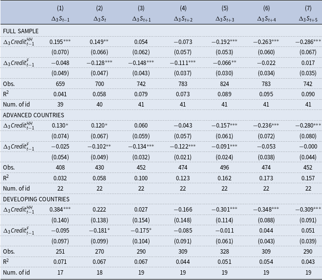
The table shows the results of the fixed-effects panel regression ${\Delta }_3S_{it+k}={\alpha }_i+{\beta }_{HH}{\Delta }_3{Credit}^{HH}_{it-1}+{\beta }_F{\Delta }_3{Credit}^F_{it-1}+u_{it+k}$
, where k = −1, 0, … 5. The dependent variable
${\Delta }_3S_{it+k}={\alpha }_i+{\beta }_{HH}{\Delta }_3{Credit}^{HH}_{it-1}+{\beta }_F{\Delta }_3{Credit}^F_{it-1}+u_{it+k}$
, where k = −1, 0, … 5. The dependent variable ${\Delta }_3S_{it+k}$
is the three-year logarithmic change in the reel services sector output level in period t + k. The independent variables
${\Delta }_3S_{it+k}$
is the three-year logarithmic change in the reel services sector output level in period t + k. The independent variables ${\Delta }_3{Credit}^{HH}_{it-1}$
and
${\Delta }_3{Credit}^{HH}_{it-1}$
and ${\Delta }_3{Credit}^F_{it-1}$
are the three-year changes in the household and non-financial firm credit to GDP ratio in period t−1, respectively. Standard errors are clustered across countries and years and given in parentheses, with ***
p
${\Delta }_3{Credit}^F_{it-1}$
are the three-year changes in the household and non-financial firm credit to GDP ratio in period t−1, respectively. Standard errors are clustered across countries and years and given in parentheses, with ***
p $\mathrm{\lt }$
0.01, **
p
$\mathrm{\lt }$
0.01, **
p $\mathrm{\lt }$
0.05, *
p
$\mathrm{\lt }$
0.05, *
p $\mathrm{\lt }$
0.1.
$\mathrm{\lt }$
0.1.
The above discussions about Table 3 showed that credit dynamics, especially household credits, can have strong negative effects on manufacturing growth over the medium run. Then, Table 4 shows the same analysis in the case of the services sector. The regression results in the upper panel show that there are positive effects of household credits in the short-run (i.e. models (1) and (2) in Table 4), whereas there are negative effects in the medium run (i.e. models (5), (6), and (7) in Table 4). So, the change in the household credit to GDP ratio leads to a rise in the services sector growth rate in the current and following periods. However, in the periods after three years, this effect turns negative, implying that a rise in the change of the household credit to GDP ratio is associated with lower growth rates. Hence, the dynamic relationship between household credits and the services sector is quite different compared to the manufacturing sector. Namely, there are boom-bust cycles in the case of the services sector, while there was only a bust period in the case of the manufacturing sector. This is a major finding of the present paper and another significant addition to the results of Mian et al. (Reference Mian, Sufi and Verner2017). It implies that the corresponding boom-bust cycles are only observed in the case of the services sector. However, the impact sizes of medium-run negative effects are relatively smaller in the services sector. For example, the regression coefficient of −0.192 in model (5) of Table 4 for the household credit implies that a one standard deviation increase in change in the household debt to GDP ratio in the last three years (i.e. 6.4% as shown in Table 1) would correspond to a 1.23 percentage point lower growth of the services sector in the following three years.
In addition to different sector-based dynamics, Table 4 shows that there are important differences between the advanced and developing country groups. It is found that the corresponding boom-bust cycles are larger in developing countries. For example, the contemporaneous effect of the change in the household credit to GDP ratio is measured by the regression coefficient of 0.130 for the advanced countries (model (1) in the middle panel of Table 4), whereas it is measured as 0.384 for the developing countries in the lower panel. Similarly, the negative growth effects in the medium run are measured with the regression coefficient of −0.157 for the developing countries (model (5) in the middle panel of Table 4), while it is measured as −0.301 for the developing countries in the lower panel. Hence, the boom-bust cycles of the services sector, which can be considered as a proxy for the non-tradable sector, seem to be more sensitive to the household credits in developing countries compared to advanced countries. However, the relevant negative medium-run effects are still smaller (in absolute value) in the services sector relative to the manufacturing sector.
Tables 3 and 4 provide evidence on the sensitivity of manufacturing and services sectors to the household and firm credits as separate regression models. However, it can be argued that the dynamics of these sectors would be closely related to each other within the same country. Then, as a robustness analysis, conducting a SUR model would be informative. In this context, Table 5 presents the results of the SUR model for the full sample of countries. The findings mainly confirm the results in the previous two tables. Namely, there is a direct negative impact of the house credits on the manufacturing growth rate both in the short run and medium run. In contrast, in the case of the services sector, there is a positive effect in the short run and a negative effect in the medium run. So, the services sector displays boom-bust cycles in its relationship with household credit. In addition, the effect sizes are much larger in the case of the manufacturing sector.
Table 5. Seemingly unrelated regression (SUR) model
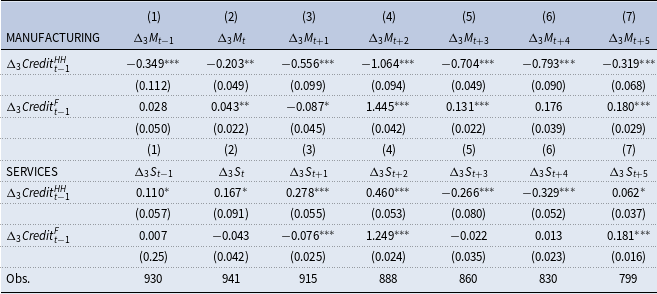
The table shows the results of the panel data seemingly unrelated regression model, where two equations ${\Delta }_3M_{it+k}={\alpha }_i+{\beta }_{HH}{\Delta }_3{Credit}^{HH}_{it-1}+{\beta }_F{\Delta }_3{Credit}^F_{it-1}+u_{it+k}$
, and
${\Delta }_3M_{it+k}={\alpha }_i+{\beta }_{HH}{\Delta }_3{Credit}^{HH}_{it-1}+{\beta }_F{\Delta }_3{Credit}^F_{it-1}+u_{it+k}$
, and ${\Delta }_3S_{it+k}={\alpha }_i+{\beta }_{HH}{\Delta }_3{Credit}^{HH}_{it-1}+{\beta }_F{\Delta }_3{Credit}^F_{it-1}+u_{it+k}$
, are jointly estimated using the SUR method. The dependent variables
${\Delta }_3S_{it+k}={\alpha }_i+{\beta }_{HH}{\Delta }_3{Credit}^{HH}_{it-1}+{\beta }_F{\Delta }_3{Credit}^F_{it-1}+u_{it+k}$
, are jointly estimated using the SUR method. The dependent variables ${\Delta }_3M_{it+k}$
and
${\Delta }_3M_{it+k}$
and ${\Delta }_3S_{it+k}$
are the three-year logarithmic changes in the reel manufacturing and services sector output levels in period t + k. The independent variables
${\Delta }_3S_{it+k}$
are the three-year logarithmic changes in the reel manufacturing and services sector output levels in period t + k. The independent variables ${\Delta }_3{Credit}^{HH}_{it-1}$
and
${\Delta }_3{Credit}^{HH}_{it-1}$
and ${\Delta }_3{Credit}^F_{it-1}$
are the three-year changes in the household and non-financial firm credit to GDP ratio in period t−1, respectively. Standard errors are clustered across countries and years and given in parentheses, with ***
p
${\Delta }_3{Credit}^F_{it-1}$
are the three-year changes in the household and non-financial firm credit to GDP ratio in period t−1, respectively. Standard errors are clustered across countries and years and given in parentheses, with ***
p $\mathrm{\lt }$
0.01, **
p
$\mathrm{\lt }$
0.01, **
p $\mathrm{\lt }$
0.05, *
p
$\mathrm{\lt }$
0.05, *
p $\mathrm{\lt }$
0.1.
$\mathrm{\lt }$
0.1.
Overall, the panel data regression results expand the findings of Mian et al. (Reference Mian, Sufi and Verner2017) in terms of sector-level dynamics and differences across advanced and developing countries. Mian et al. (Reference Mian, Sufi and Verner2017) show that household credits create business cycles in the real GDP in the form of positive short-run effects and negative long-run effects. The present paper shows that these business cycles mainly arise from the boom-bust cycles in the services sector. In the case of the manufacturing sector, there are no boom periods due to the household credit rise. In addition, the manufacturing growth-credit nexus does not differ across the advanced and developing countries. However, in the case of the boom-bust cycles in the services sector, these cycles are larger in magnitude in developing countries. Moreover, the negative medium-run effects of the household credit are larger in magnitude in the manufacturing sector relative to the services sector. Therefore, the present paper provides richer sets of results and dynamics in the finance-growth nexus in terms of sector-level and cross-country differences.
While the present paper documents the presence of heterogenous credit-driven business cycles across countries and sectors, it does not identify the sources of these heterogeneities. As discussed in the introduction section, there can be different theoretical mechanisms justifying heterogenous business cycles. For instance, in developing countries, relatively low levels of financial development and weak contract enforceability can result in greater boom-bust cycles [Ranciere et al. (Reference Ranciere, Tornell and Westermann2008)]. Similarly, the presence of foreign currency borrowing and pecuniary externalities in these countries can significantly raise the credit sensitivity of output [Bianchi (Reference Bianchi2011)]. Concerning the disparities in credit-driven cycles between the manufacturing and service sectors, similar arguments can be made, with financial constraints being more binding in the services sector [Tornell and Westermann (Reference Tornell and Westermann2005); Gunay and Kilinc (2015)], resulting in credit-driven boom-bust cycles in this sector. Another possible mechanism is credit booms (particularly household credit), which can lead to currency appreciation [Bahadir and Gumus (Reference Bahadir and Gumus2016)], with negative effects on manufacturing sector growth [Rodrik (Reference Rodrik2008)]. As a result, the negative medium-term effects of household credit in the manufacturing sector may be greater than in the services sector. Other factors that can cause differential sector-level sensitivities include different labor intensities, input-output linkages, product differentiation, and returns to scale. For example, external finance dependence can vary across sectors [Rajan and Zinagles (Reference Rajan and Zingales1998)], and these differences can affect the credit sensitivity of the sectors. Overall, the heterogeneous credit-driven business cycles across countries and sectors can be substantiated using various theoretical mechanisms, and the current paper strongly establishes the relevant empirical regularities using a large dataset.
6. Robustness analysis
This section conducts various robustness analyses to check if the new results continue to hold under new specifications, the inclusion of new variables, and the use of new datasets. Given that credit variables are the main variables of interest in the present study, whether the findings are robust to the banking or financial crises is a relevant robustness question. Namely, the results might be driven by credit crises and periods, and it is possible that in non-crisis periods, there are no boom-bust cycles driven by credits. For example, Tornell and Westermann (Reference Tornell and Westermann2005) show the existence of boom-bust cycles in N/T ratio around the crisis periods. A detailed robustness analysis to check the possible role of the crises would be to include the crisis-year dummies and their interactions with the credit variables. The relevant information on banking and financial crisis is obtained from the Behavioral Finance and Financial Stability (2022) at the Harvard Business School. Then, the relevant crisis dummies, as well as their interactions with credit variables, are included as additional regressors in the estimations. The relevant results are presented in Tables 6 and 7.
Table 6. Fixed-effects regression of the real manufacturing output growth on household and firm credit with banking crisis
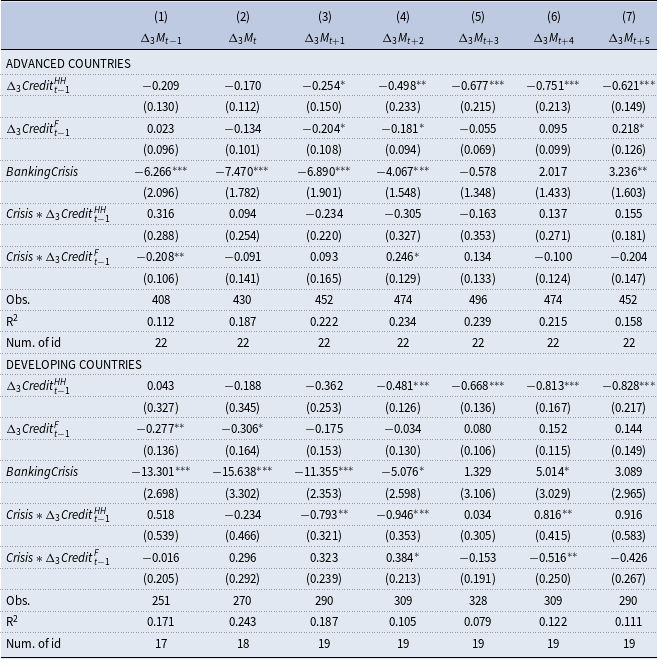
The table shows the results of the fixed-effects panel regression ${\Delta }_3M_{it+k}={\alpha }_i+{\beta }_{HH}{\Delta }_3{Credit}^{HH}_{it-1}+{\beta }_F{\Delta }_3{Credit}^F_{it-1}+u_{it+k}$
, where k = −1, 0, … 5. The dependent variable
${\Delta }_3M_{it+k}={\alpha }_i+{\beta }_{HH}{\Delta }_3{Credit}^{HH}_{it-1}+{\beta }_F{\Delta }_3{Credit}^F_{it-1}+u_{it+k}$
, where k = −1, 0, … 5. The dependent variable ${\Delta }_3M_{it+k}$
is the three-year logarithmic change in the real manufacturing level in period t + k. The independent variables
${\Delta }_3M_{it+k}$
is the three-year logarithmic change in the real manufacturing level in period t + k. The independent variables ${\Delta }_3{Credit}^{HH}_{it-1}$
and
${\Delta }_3{Credit}^{HH}_{it-1}$
and ${\Delta }_3{Credit}^F_{it-1}$
are the three-year changes in the household and non-financial firm credit to GDP ratio in period t−1, respectively. Standard errors are clustered across countries and years and given in parentheses, with ***
p
${\Delta }_3{Credit}^F_{it-1}$
are the three-year changes in the household and non-financial firm credit to GDP ratio in period t−1, respectively. Standard errors are clustered across countries and years and given in parentheses, with ***
p $\mathrm{\lt }$
0.01, **
p
$\mathrm{\lt }$
0.01, **
p $\mathrm{\lt }$
0.05, *
p
$\mathrm{\lt }$
0.05, *
p $\mathrm{\lt }$
0.1.
$\mathrm{\lt }$
0.1.
Table 7. Fixed-effects regression of the real services growth on household and firm credit with banking crisis variables
The table shows the results of the fixed-effects panel regression ${\Delta }_3S_{it+k}={\alpha }_i+{\beta }_{HH}{\Delta }_3{Credit}^{HH}_{it-1}+{\beta }_F{\Delta }_3{Credit}^F_{it-1}+u_{it+k}$
, where k = −1, 0, … 5. The dependent variable
${\Delta }_3S_{it+k}={\alpha }_i+{\beta }_{HH}{\Delta }_3{Credit}^{HH}_{it-1}+{\beta }_F{\Delta }_3{Credit}^F_{it-1}+u_{it+k}$
, where k = −1, 0, … 5. The dependent variable ${\Delta }_3S_{it+k}$
is the three-year logarithmic change in the real services level in period t + k. The independent variables
${\Delta }_3S_{it+k}$
is the three-year logarithmic change in the real services level in period t + k. The independent variables ${\Delta }_3{Credit}^{HH}_{it-1}$
and
${\Delta }_3{Credit}^{HH}_{it-1}$
and ${\Delta }_3{Credit}^F_{it-1}$
are the three-year changes in the household and non-financial firm credit to GDP ratio in period t−1, respectively. Standard errors are clustered across countries and years and given in parentheses, with ***
p
${\Delta }_3{Credit}^F_{it-1}$
are the three-year changes in the household and non-financial firm credit to GDP ratio in period t−1, respectively. Standard errors are clustered across countries and years and given in parentheses, with ***
p $\mathrm{\lt }$
0.01, **
p
$\mathrm{\lt }$
0.01, **
p $\mathrm{\lt }$
0.05, *
p
$\mathrm{\lt }$
0.05, *
p $\mathrm{\lt }$
0.1.
$\mathrm{\lt }$
0.1.
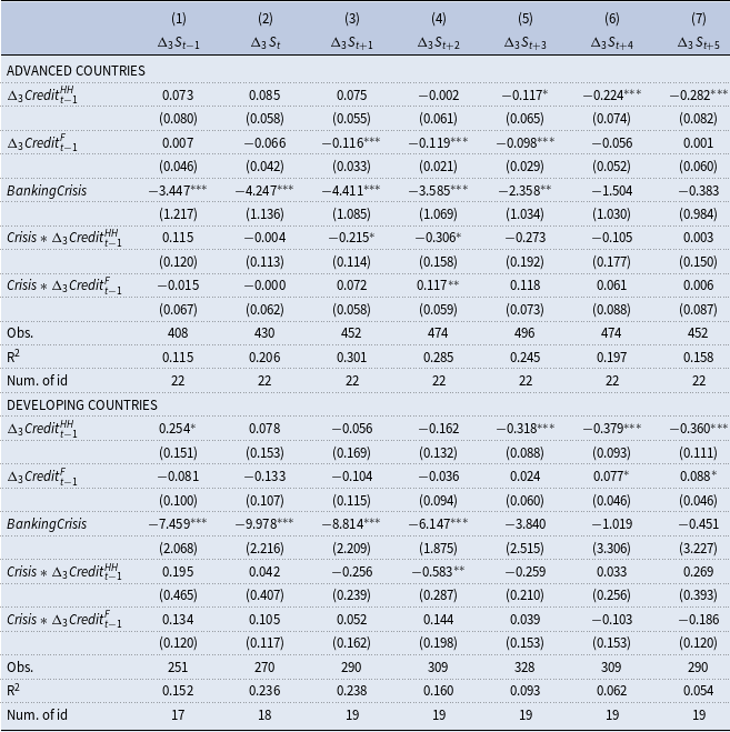
The results in Table 6 show that crisis dummies have negative effects on the manufacturing output growth in the short run for both advanced and developing countries, while their impacts disappear in the medium run. In addition, the negative effects are stronger in the case of developing countries. Moreover, the interaction terms with the household credits are statistically significant in certain specifications for developing countries, implying that the negative impacts of household credits are amplified during crisis periods. However, no similar interaction effects of household credits for the manufacturing sector are found in the case of advanced countries. This finding also supports the general result that credit-driven cycles differ between advanced and developing countries. Table 7 documents similar findings in the case of the services sector as well. Namely, the crises produce negative short-term effects on the service sector growth, while these effects disappear over the medium run. In addition, the interactions between crisis dummies and household credit point to amplified medium-run negative effects of household credits during crises. Moreover, household credits still produce negative medium-run effects (unconditional on crises) on the services sector. However, one important difference between Tables 6 and 7 is that the services sector in developing countries experiences positive short-term effects of household credits. So, the services sector experiences boom-bust cycles driven by housing credits in developing countries. Based on Tables 6 and 7, it can be argued that even after controlling these crisis effects, the main results continue to hold in the sense that developing countries and services sectors display boom-bust cycles, while the negative medium-run effects of household credits are stronger in the manufacturing sector relative to the services sector.
Another robustness analysis in the study is to exclude the global financial crisis and the following years from the empirical analysis. Mian et al. (Reference Mian, Sufi and Verner2017) find that the relevant results can be sensitive to this exclusion. In the present dataset, the relevant fixed-effects regression results are presented in Tables 12, 13, and 14, for GDP, the manufacturing sector, and the services sector, respectively. The results show that developing countries display higher sensitivity to household credits relative to advanced countries. In addition, it is found that the services sector in developing countries documents boom-bust cycles (i.e. short-run positive effects of household credits and negative medium-run effects), while no credit-driven cycles are observed in advanced countries or the manufacturing sector. Still, the negative medium-run effects of household credits are larger in the manufacturing sector. Hence, the exclusion of the global financial crisis does not change the main results of the present study.
Another robustness analysis is the inclusion of additional macroeconomic variables in the main regression equations. In this context, Tables 15, 16, and 17 (for GDP, the manufacturing sector, and the services sector, respectively) present the fixed-effects regression results with the control variables of government consumption to GDP ratio, investments to GDP ratio, current account to GDP ratio, the unemployment rate, and the inflation rate. The regression results imply that government consumption and inflation are associated with lower GDP growth rates, while investments are associated with higher GDP growth rates in the full sample. The results continue to hold in the sense that developing countries display household credit-driven boom-bust cycles in contrast to advanced countries. In addition, the responsiveness of the manufacturing sector is higher in the medium run compared to the services sector. However, the sizes of regression coefficients for credit variables decline (in absolute value) to some extent when macroeconomic variables are included in the regression models. For example, the impact of household credits in model (7) in Table 2 was −0.373 for the full sample, −0.356 for advanced countries, and −0.431 for developing countries. These coefficients become −0.252, −0.223, and −0.263, respectively, in Table 15. Hence, the explanatory power of credit variables declines to some extent, while their impacts are still statistically and economically significant. In addition to including additional macroeconomic variables, Mian et al. (Reference Mian, Sufi and Verner2017) also include distributed lags to control for the possibility of mean reversion in time-series variables. The present paper also follows the same approach and includes the lags of the dependent variables in the regression models from (4) to (7). The corresponding results are presented in Tables 18, 19, and 20 for GDP, the manufacturing sector, and the services sector, respectively. The results are also robust to this extension in the regression model. Tables 21, 22, and 23 provide more detailed results in the case of the regression models with the banking crisis variables.
As a further robustness analysis, Tables 24, 25, and 26 combine the above extensions in the same regression models in terms of control variables, distributed lags, crisis dummies, and crisis interactions with credit variables. The results are robust to these specifications as well. Finally, as another robustness, Tables 27, 28, and 29 utilize one-period differences instead of three-period differences.
One possible issue with the above results is that the classification of the services sector in the World Bank database includes the financial sector. Then, it is likely that the credit cycles would be directly reflected in the dynamics of the services sector. As a robustness analysis, it would be informative to exclude the financial sector from the analysis. For this purpose, a new dataset on sector-level output and employment levels is obtained from the 10-sector database of the Groningen Growth and Development Centre (GGDC) (2022). From this database, the services sector is constructed as the sum of (i) construction, (ii) trade, restaurants and hotels, and (iii) transport, storage, and communication. In this classification, the sectors of finance, insurance, real estate, business services, government services, and community, social and personal services are not included in the services definition. Then, the manufacturing data are also obtained from the same database to produce comparable results. We repeat the same estimations with this new dataset and present the results in Tables 30 and 31 for the manufacturing and services sectors, respectively. One shortcoming, in this case, is that the number of countries in the sample declines from 41 to 19 (10 advanced countries and 9 developing countries). The results show that developing countries and the manufacturing sector are more sensitive to household credits in the medium run. However, the boom effects in the short run are not observed in the services sector. Finally, with the new dataset, it is also possible to examine the possible credit effects on sector-level employment growth as the dependent variables. The relevant regression results are presented in Tables 32 and 33. The results show that household credits affect manufacturing employment negatively over the medium run in advanced countries and in both short and medium runs in developing countries. In addition, the negative impact is larger in developing countries. In the case of services employment, household credits produce negative effects for developing countries, while they produce short-run positive and medium-run negative effects for advanced countries. Similar effects of boom-bust cycles in services employment are also obtained in response to the corporate credits. These analyses can be extended for different sector-level variables such as investments and exports in future research.
7. Conclusion
This paper has examined the relationship between credit developments and sector-level output dynamics in a large sample of 41 advanced and developing countries. The existing literature shows that changes in the household credits to GDP ratio are associated with boom-bust cycles in the aggregate output, whereas firm credits do not produce such output dynamics. Namely, when there is an increase in the household credit to GDP ratio, the real GDP growth rises contemporaneously while it declines in the following three or four years. Mian et al. (Reference Mian, Sufi and Verner2017) interpret these boom-bust output dynamics or real business cycles associated with household credit as indications of positive supply credit shocks and overoptimistic expectations about future economic activity. The present paper expands these findings in terms of advanced versus developing countries and manufacturing versus services sectors.
The new findings indicate that the resulting boom-bust cycles in the aggregate output are generally observed in the sample of developing countries, with no similar dynamics in the advanced countries. Hence, the credit market mechanisms seem to differ across country groups. As another major finding, the paper shows that the boom-bust cycles are generated mainly in the services sector, with no similar dynamics in the services sector. However, the medium-run negative effects are stronger in the manufacturing sector. These findings matter for the modeling of the financial frictions in developing versus advanced countries, as well as mechanisms affecting manufacturing versus services sectors or tradable versus non-tradable sectors. For example, Schneider and Tornell (Reference Schneider and Tornell2004) show that the presence of currency mismatches and systemic bailout guarantees can generate asymmetric responses of tradable versus non-tradable sectors to credit developments for emerging countries. Therefore, the findings of the present paper provide valuable empirical inputs to the literature on the finance-growth nexus in terms of the boom-bust cycles or real business cycles generated by credit developments across advanced versus developing countries and tradable versus non-tradable sectors.
The above discussions show that the extension of the literature on the credit growth nexus in terms of heterogenous credit-driven business cycles across countries and sectors is of high importance for the relevant literature. While the present paper does not identify the sources of these heterogeneous cycles, their presence implies that researchers and policymakers need to take these differences into account. For example, recent decades have experienced major structural changes in many countries where the share of the manufacturing sector declined to a large extent [Matsuyama (Reference Matsuyama2009), while the tradability of services increased significantly [Francois and Hoekman (Reference Francois and Hoekman2010)]. The findings of the present paper imply that credit market developments can be important factors for the structural changes in the economy. Then, identifying the sources of these heterogenous credit-driven business cycles and their association with structural changes in the relevant countries becomes important research questions for future research. By collecting more detailed sector-level or firm-level data, it can become possible to recover the underlying mechanisms of sectoral heterogeneity in credit sensitivities.
A. Appendix I: Panel VAR analysis
An empirical strategy to see the dynamic relationship between credits and sector-level outputs is to use the panel VAR methods. In addition to the single-equation panel data methods, the present study also employs panel VAR methods, which allows the identification of the credit-output relationship in a more dynamic way over both short run and medium/long run. In this context, the panel VAR approach of Love and Zicchino (Reference Love and Zicchino2006) is followed. The corresponding VAR equation is given as follows:
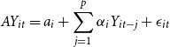 \begin{equation} AY_{it}=a_{i}+\sum ^{p}_{j=1}\alpha _{i}Y_{it-j}+\epsilon _{it} \end{equation}
In the above equation, the country fixed-effects are controlled by $a_i$
, while
$a_i$
, while $\epsilon _it$
is the vector of structural shocks with the following properties
$\epsilon _it$
is the vector of structural shocks with the following properties $E[\epsilon _{it}\epsilon ^{\prime}_{it}]=I$
and
$E[\epsilon _{it}\epsilon ^{\prime}_{it}]=I$
and $E[\epsilon _{t}\epsilon ^{\prime}_{s}]=0$
. The optimal lag length is chosen according to the model selection criteria of Andrews and Lu (Reference Andrews and Lu2001) for GMM estimations in panel data using the Akaike information criteria, the Bayesian information criteria, and the Hannan-Quinn information criteria. The reduced-form VAR equation is given as follows:
$E[\epsilon _{t}\epsilon ^{\prime}_{s}]=0$
. The optimal lag length is chosen according to the model selection criteria of Andrews and Lu (Reference Andrews and Lu2001) for GMM estimations in panel data using the Akaike information criteria, the Bayesian information criteria, and the Hannan-Quinn information criteria. The reduced-form VAR equation is given as follows:
 \begin{equation} Y_{it}=c_{i}+\sum ^{p}_{j=1}\delta _{i}Y_{it-j}+u_{it} \end{equation}
In the transformation of the VAR system, the following equalities are used: $S=A^{-1}$
,
$S=A^{-1}$
, $c_{i}=Sa_{i}$
,
$c_{i}=Sa_{i}$
, $\delta _{i}=S\alpha _{i}$
, and
$\delta _{i}=S\alpha _{i}$
, and $u_{it}=S\epsilon _{it}$
. The structural shocks are identified using the Cholesky decomposition where the structural shocks are mapped into the reduced-form shocks using the S matrix with the following property
$u_{it}=S\epsilon _{it}$
. The structural shocks are identified using the Cholesky decomposition where the structural shocks are mapped into the reduced-form shocks using the S matrix with the following property $E[u_{it}u^{\prime}_{it}]=SS^{\prime}=\Sigma$
. This model is estimated using the GMM approach with forward orthogonal deviation. In this context, the impulse response functions become valuable to see the dynamics relationship between output and credit variables. The confidence intervals of the impulse response functions are estimated using the Monte Carlo simulation and bootstrap resampling methods [Love and Zicchino (Reference Love and Zicchino2006)].
$E[u_{it}u^{\prime}_{it}]=SS^{\prime}=\Sigma$
. This model is estimated using the GMM approach with forward orthogonal deviation. In this context, the impulse response functions become valuable to see the dynamics relationship between output and credit variables. The confidence intervals of the impulse response functions are estimated using the Monte Carlo simulation and bootstrap resampling methods [Love and Zicchino (Reference Love and Zicchino2006)].
The results of the panel VAR model are examined in terms of impulse responses. Four lags are selected in the estimations and the first panel VAR model includes the following variables: $\triangle Household Credit/GDP_{t}$
,
$\triangle Household Credit/GDP_{t}$
, $\triangle Firm Credit/GDP_{t}$
,
$\triangle Firm Credit/GDP_{t}$
, $\triangle Ln(GDP_{t})$
. The model satisfies the necessary stability conditions of Love and Zicchino (Reference Love and Zicchino2006). The corresponding impulse responses of the real GDP growth to the household and firm credit shocks are presented in Figure 5. The graph shows the impulse response lines and the 90% confidence intervals estimated by the Monte Carlo simulation and bootstrap resampling methods. It is seen that in the case of the aggregate output, a rise in the change of the firm credit to GDP ratio leads to a slight decline in the real output growth rate, which is statistically significant for around four years. This finding is consistent with the panel data regression results in Table 2. Then, in the case of the household credit, a rise in its change as a ratio to GDP is associated with an increase in the output growth in the short run, whereas it leads to lower output growth in the medium run. Hence, the dynamics of the household credit create boom-bust cycles in the aggregate output. This finding is also consistent with the panel data regression results in Table 2, which finds positive short-run effects and negative medium-run effects of household credit. This finding is also the main result of the paper by Mian et al. (Reference Mian, Sufi and Verner2017). Overall, impulse response functions in Figure 5 provide supportive evidence on the boom-bust creating capacity of household credits for the aggregate economic activity. When the ordering of variables is changed as a robustness exercise, the impulse response functions stay very similar, showing the robustness of findings to the ordering of variables.
$\triangle Ln(GDP_{t})$
. The model satisfies the necessary stability conditions of Love and Zicchino (Reference Love and Zicchino2006). The corresponding impulse responses of the real GDP growth to the household and firm credit shocks are presented in Figure 5. The graph shows the impulse response lines and the 90% confidence intervals estimated by the Monte Carlo simulation and bootstrap resampling methods. It is seen that in the case of the aggregate output, a rise in the change of the firm credit to GDP ratio leads to a slight decline in the real output growth rate, which is statistically significant for around four years. This finding is consistent with the panel data regression results in Table 2. Then, in the case of the household credit, a rise in its change as a ratio to GDP is associated with an increase in the output growth in the short run, whereas it leads to lower output growth in the medium run. Hence, the dynamics of the household credit create boom-bust cycles in the aggregate output. This finding is also consistent with the panel data regression results in Table 2, which finds positive short-run effects and negative medium-run effects of household credit. This finding is also the main result of the paper by Mian et al. (Reference Mian, Sufi and Verner2017). Overall, impulse response functions in Figure 5 provide supportive evidence on the boom-bust creating capacity of household credits for the aggregate economic activity. When the ordering of variables is changed as a robustness exercise, the impulse response functions stay very similar, showing the robustness of findings to the ordering of variables.
While Figure 5 confirms the findings of Mian et al. (Reference Mian, Sufi and Verner2017) and the new panel data regression results in Table 2, the main objective of the present paper is to decompose the aggregate output dynamics into sector-level effects. In this context, Figure 6 shows the impulse responses of real growth rates to the changes in the firm and household credits to GDP ratios. The upper panel shows the responses of the services and manufacturing sectors to a rise in the change of firm credit to GDP ratio. It is found that both services and manufacturing growth rates decline in response to the rise in the firm credit, while these negative effects are relatively smaller (in absolute value) in the case of the services sector. The panel data regression results of Tables 3 and 4 also confirm these findings. Table 4 finds that the peak negative effect of the firm credits on the services sector is −0.148 in model (3), while Table 3 shows that the peak negative effect on the manufacturing sector is −0.272 in model (2). Hence, consistent with the results in Table 2 and Figure 5, as well as the findings of Mian et al. (Reference Mian, Sufi and Verner2017), the movements in the change of the firm credits to GDP do not create boom-bust cycles in the aggregate output or the sector-level outputs.
In contrast to the relatively small and one-directional effects (i.e. only negative effects) of the firm credits on economic activity and sector-level outputs, the lower panel of Figure 6 shows that household credits generate larger and two-directional effects (i.e. both positive and negative effects or boom-bust cycles) on sector-level outputs. In the case of the services sector, there are small positive effects in the short run, whereas the medium-run effects are negative. These results are consistent with the findings of the panel data regressions in Table 4. The results showed that there are positive regression coefficients of the household credits on the services sector in the short-run models (1) and (2), whereas there are negative effects in the medium-run models (5), (6), and (7).

Figure 5. Impulse responses of real GDP to the household and firm credit shocks from the panel VAR model.

Figure 6. Impulse responses of sector-level outputs to the household and firm credit shocks with 1-year differences.
In the case of the manufacturing sector, the lower panel of Figure 6 shows that the household credits create larger boom-bust cycles with larger positive effects in the short run and larger negative effects in the medium run. These larger negative medium-run effects of the household credits are also observed in the panel data regression coefficients of Table 3. For example, it is found that the regression coefficient of the household credits in the model (5) of Table 3 was −0.701 for the manufacturing sector compared to a regression coefficient of -0.192 in the same model of Table 4 for the services sector. Hence, the lower panel of Figure 6 shows similar differential medium-run effects of the change in the household credits to GDP ratio for the services and manufacturing sectors. However, the short-run positive effects of the household credits on the manufacturing output are a different result from the findings of the panel data regressions. This finding might arise from the different formats of variables (i.e. three-year differences in the case of panel data and one-year differences in the case of panel VAR). As a robustness analysis, the VAR analysis is repeated with three-year differences in the relevant dependent and independent variables. In this case, the optimal lag length is selected as two based on the relevant statistics. The corresponding impulse response functions are presented in Figure 7.
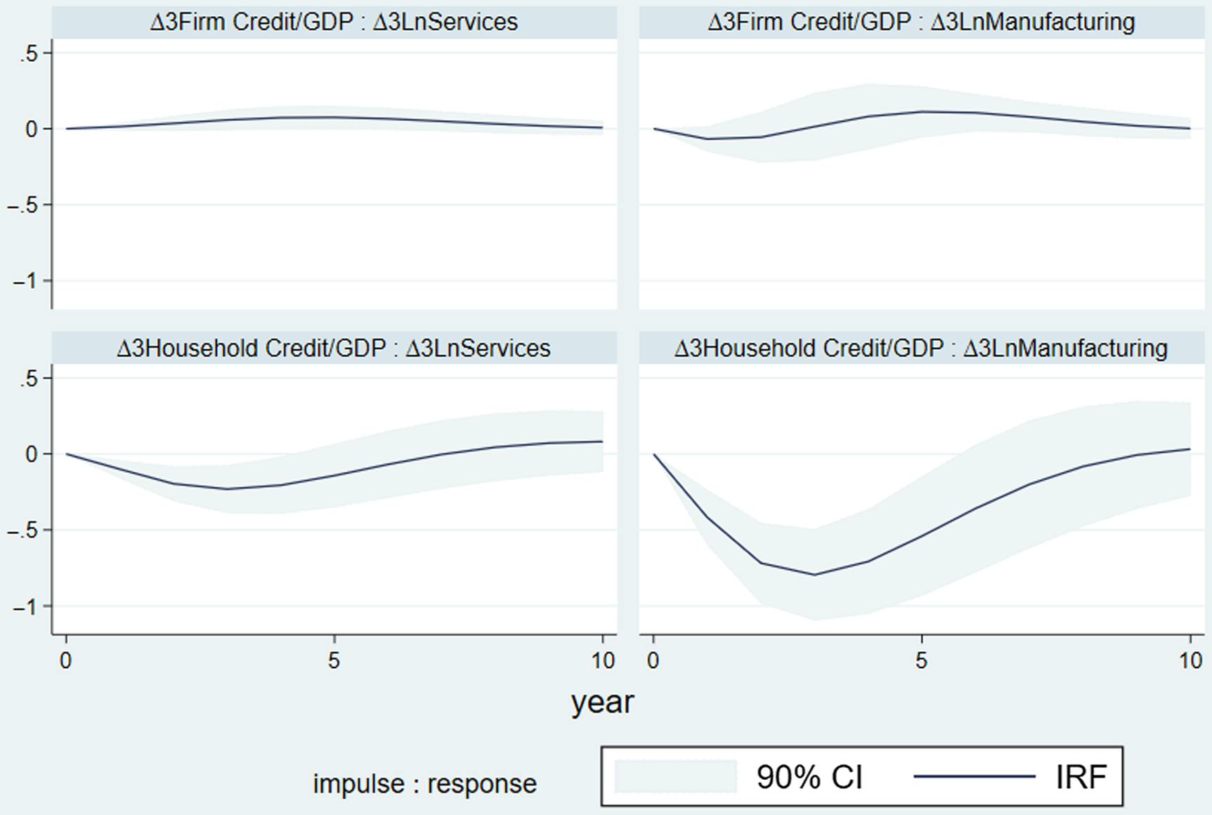
Figure 7. Shows that both manufacturing and services sectors are negatively affected by the changes in the household credits over the medium run. In addition, the responsiveness of the manufacturing sector is higher than the services sector. In contrast, the impacts of the firm credits are not statistically significant for both sectors. When the impulse response functions are compared between Figures 6 and 7, some differences are found. For example, the boom periods of household credit in both sectors are not observed when three-year differences are utilized. These results mostly confirm the medium-run effects documented in columns 4 to 7 in the relevant panel regression tables. Overall, the panel VAR results also display important differences in the sector-level sensitivities to credit developments.
B. Appendix II: Additional tables
Table 8. Summary statistics for advanced and developing countries

Table 9. Fixed-effects regression of the real output growth on private sector credit
The table shows the results of the fixed-effects panel regression ${\Delta }_3Y_{it+k}={\alpha }_i+{\beta }_C{\Delta }_3{Credit}_{t-1}+u_{it+k}$
, where k = −1, 0, … 5. The dependent variable
${\Delta }_3Y_{it+k}={\alpha }_i+{\beta }_C{\Delta }_3{Credit}_{t-1}+u_{it+k}$
, where k = −1, 0, … 5. The dependent variable ${\Delta }_3Y_{it+k}$
is the three-year logarithmic change in the reel GDP level in period t + k. The independent variable
${\Delta }_3Y_{it+k}$
is the three-year logarithmic change in the reel GDP level in period t + k. The independent variable ${\Delta }_3{Credit}_{t-1}$
is the three-year change in the private sector credit (i.e. households and non-financial firms) to GDP ratio in period t−1. Robust standard errors are given in parentheses, with ***
p
${\Delta }_3{Credit}_{t-1}$
is the three-year change in the private sector credit (i.e. households and non-financial firms) to GDP ratio in period t−1. Robust standard errors are given in parentheses, with ***
p $\mathrm{\lt }$
0.01, **
p
$\mathrm{\lt }$
0.01, **
p $\mathrm{\lt }$
0.05, *
p
$\mathrm{\lt }$
0.05, *
p $\mathrm{\lt }$
0.1.
$\mathrm{\lt }$
0.1.
Table 10. Fixed-Effects regression of the real manufacturing growth on private sector credit

The table shows the results of the fixed-effects panel regression ${\Delta }_3M_{it+k}={\alpha }_i+{\beta }_C{\Delta }_3{Credit}_{t-1}+u_{it+k}$
, where k = −1, 0, … 5. The dependent variable
${\Delta }_3M_{it+k}={\alpha }_i+{\beta }_C{\Delta }_3{Credit}_{t-1}+u_{it+k}$
, where k = −1, 0, … 5. The dependent variable ${\Delta }_3M_{it+k}$
is the three-year logarithmic change in the reel manufacturing sector output level in period t + k. The independent variable
${\Delta }_3M_{it+k}$
is the three-year logarithmic change in the reel manufacturing sector output level in period t + k. The independent variable ${\Delta }_3{Credit}_{t-1}$
is the three-year change in the private sector credit (i.e. households and non-financial firms) to GDP ratio in period t−1. Robust standard errors are given in parentheses, with ***
p
${\Delta }_3{Credit}_{t-1}$
is the three-year change in the private sector credit (i.e. households and non-financial firms) to GDP ratio in period t−1. Robust standard errors are given in parentheses, with ***
p $\mathrm{\lt }$
0.01, **
p
$\mathrm{\lt }$
0.01, **
p $\mathrm{\lt }$
0.05, *
p
$\mathrm{\lt }$
0.05, *
p $\mathrm{\lt }$
0.1.
$\mathrm{\lt }$
0.1.
Table 11. Fixed-effects regression of the real services growth on private sector credit

The table shows the results of the fixed-effects panel regression ${\Delta }_3S_{it+k}={\alpha }_i+{\beta }_C{\Delta }_3{Credit}_{t-1}+u_{it+k}$
, where k = −1, 0, … 5. The dependent variable
${\Delta }_3S_{it+k}={\alpha }_i+{\beta }_C{\Delta }_3{Credit}_{t-1}+u_{it+k}$
, where k = −1, 0, … 5. The dependent variable ${\Delta }_3S_{it+k}$
is the three-year logarithmic change in the reel services sector output level in period t+k. The independent variable
${\Delta }_3S_{it+k}$
is the three-year logarithmic change in the reel services sector output level in period t+k. The independent variable ${\Delta }_3{Credit}_{t-1}$
is the three-year change in the private sector credit (i.e. households and non-financial firms) to GDP ratio in period t−1. Robust standard errors are given in parentheses, with ***
p
${\Delta }_3{Credit}_{t-1}$
is the three-year change in the private sector credit (i.e. households and non-financial firms) to GDP ratio in period t−1. Robust standard errors are given in parentheses, with ***
p $\mathrm{\lt }$
0.01, **
p
$\mathrm{\lt }$
0.01, **
p $\mathrm{\lt }$
0.05, *
p
$\mathrm{\lt }$
0.05, *
p $\mathrm{\lt }$
0.1.
$\mathrm{\lt }$
0.1.
Table 12. Fixed-effects regression of the real output growth on household and firm credit for the periods before the global financial crisis

The table shows the results of the fixed-effects panel regression ${\Delta }_3Y_{it+k}={\alpha }_i+{\beta }_{HH}{\Delta }_3{Credit}^{HH}_{it-1}+{\beta }_F{\Delta }_3{Credit}^F_{it-1}+u_{it+k}$
, where k = −1, 0, … 5. The dependent variable
${\Delta }_3Y_{it+k}={\alpha }_i+{\beta }_{HH}{\Delta }_3{Credit}^{HH}_{it-1}+{\beta }_F{\Delta }_3{Credit}^F_{it-1}+u_{it+k}$
, where k = −1, 0, … 5. The dependent variable ${\Delta }_3Y_{it+k}$
is the three-year logarithmic change in the real GDP level in period t + k. The independent variables
${\Delta }_3Y_{it+k}$
is the three-year logarithmic change in the real GDP level in period t + k. The independent variables ${\Delta }_3{Credit}^{HH}_{it-1}$
and
${\Delta }_3{Credit}^{HH}_{it-1}$
and ${\Delta }_3{Credit}^F_{it-1}$
are the three-year changes in the household and non-financial firm credit to GDP ratio in period t−1, respectively. Standard errors are clustered across countries and years and given in parentheses, with ***
p
${\Delta }_3{Credit}^F_{it-1}$
are the three-year changes in the household and non-financial firm credit to GDP ratio in period t−1, respectively. Standard errors are clustered across countries and years and given in parentheses, with ***
p $\mathrm{\lt }$
0.01, **
p
$\mathrm{\lt }$
0.01, **
p $\mathrm{\lt }$
0.05, *
p
$\mathrm{\lt }$
0.05, *
p $\mathrm{\lt }$
0.1.
$\mathrm{\lt }$
0.1.
Table 13. Fixed-effects regression of the real manufacturing growth on household and firm credit for the periods before the global financial crisis

The table shows the results of the fixed-effects panel regression ${\Delta }_3M_{it+k}={\alpha }_i+{\beta }_{HH}{\Delta }_3{Credit}^{HH}_{it-1}+{\beta }_F{\Delta }_3{Credit}^F_{it-1}+u_{it+k}$
, where k = −1, 0, … 5. The dependent variable
${\Delta }_3M_{it+k}={\alpha }_i+{\beta }_{HH}{\Delta }_3{Credit}^{HH}_{it-1}+{\beta }_F{\Delta }_3{Credit}^F_{it-1}+u_{it+k}$
, where k = −1, 0, … 5. The dependent variable ${\Delta }_3M_{it+k}$
is the three-year logarithmic change in the real manufacturing sector output level in period t + k. The independent variables
${\Delta }_3M_{it+k}$
is the three-year logarithmic change in the real manufacturing sector output level in period t + k. The independent variables ${\Delta }_3{Credit}^{HH}_{it-1}$
and
${\Delta }_3{Credit}^{HH}_{it-1}$
and ${\Delta }_3{Credit}^F_{it-1}$
are the three-year changes in the household and non-financial firm credit to GDP ratio in period t−1, respectively. Standard errors are clustered across countries and years and given in parentheses, with ***
p
${\Delta }_3{Credit}^F_{it-1}$
are the three-year changes in the household and non-financial firm credit to GDP ratio in period t−1, respectively. Standard errors are clustered across countries and years and given in parentheses, with ***
p $\mathrm{\lt }$
0.01, **
p
$\mathrm{\lt }$
0.01, **
p $\mathrm{\lt }$
0.05, *
p
$\mathrm{\lt }$
0.05, *
p $\mathrm{\lt }$
0.1.
$\mathrm{\lt }$
0.1.
Table 14. Fixed-effects regression of the real services growth on household and firm credit for the periods before the global financial crisis

The table shows the results of the fixed-effects panel regression ${\Delta }_3S_{it+k}={\alpha }_i+{\beta }_{HH}{\Delta }_3{Credit}^{HH}_{it-1}+{\beta }_F{\Delta }_3{Credit}^F_{it-1}+u_{it+k}$
, where k = −1, 0, … 5. The dependent variable
${\Delta }_3S_{it+k}={\alpha }_i+{\beta }_{HH}{\Delta }_3{Credit}^{HH}_{it-1}+{\beta }_F{\Delta }_3{Credit}^F_{it-1}+u_{it+k}$
, where k = −1, 0, … 5. The dependent variable ${\Delta }_3S_{it+k}$
is the three-year logarithmic change in the real services sector output level in period t + k. The independent variables
${\Delta }_3S_{it+k}$
is the three-year logarithmic change in the real services sector output level in period t + k. The independent variables ${\Delta }_3{Credit}^{HH}_{it-1}$
and
${\Delta }_3{Credit}^{HH}_{it-1}$
and ${\Delta }_3{Credit}^F_{it-1}$
are the three-year changes in the household and non-financial firm credit to GDP ratio in period t−1, respectively. Standard errors are clustered across countries and years and given in parentheses, with ***
p
${\Delta }_3{Credit}^F_{it-1}$
are the three-year changes in the household and non-financial firm credit to GDP ratio in period t−1, respectively. Standard errors are clustered across countries and years and given in parentheses, with ***
p $\mathrm{\lt }$
0.01, **
p
$\mathrm{\lt }$
0.01, **
p $\mathrm{\lt }$
0.05, *
p
$\mathrm{\lt }$
0.05, *
p $\mathrm{\lt }$
0.1.
$\mathrm{\lt }$
0.1.
Table 15. Fixed-effects regression of the real output growth on household and firm credit with control variables

The table shows the results of the fixed-effects panel regression ${\Delta }_3Y_{it+k}={\alpha }_i+{\beta }_{HH}{\Delta }_3{Credit}^{HH}_{it-1}+{\beta }_F{\Delta }_3{Credit}^F_{it-1}+\gamma{Control\ Variables}_{it-1}+u_{it+k}$
, where k = −1, 0, … 5. The dependent variable
${\Delta }_3Y_{it+k}={\alpha }_i+{\beta }_{HH}{\Delta }_3{Credit}^{HH}_{it-1}+{\beta }_F{\Delta }_3{Credit}^F_{it-1}+\gamma{Control\ Variables}_{it-1}+u_{it+k}$
, where k = −1, 0, … 5. The dependent variable ${\Delta }_3Y_{it+k}$
is the three-year logarithmic change in the real GDP level in period t + k. The independent variables
${\Delta }_3Y_{it+k}$
is the three-year logarithmic change in the real GDP level in period t + k. The independent variables ${\Delta }_3{Credit}^{HH}_{it-1}$
and
${\Delta }_3{Credit}^{HH}_{it-1}$
and ${\Delta }_3{Credit}^F_{it-1}$
are the three-year changes in the household and non-financial firm credit to GDP ratio in period t−1, respectively. Standard errors are clustered across countries and years and given in parentheses, with ***
p
${\Delta }_3{Credit}^F_{it-1}$
are the three-year changes in the household and non-financial firm credit to GDP ratio in period t−1, respectively. Standard errors are clustered across countries and years and given in parentheses, with ***
p $\mathrm{\lt }$
0.01, **
p
$\mathrm{\lt }$
0.01, **
p $\mathrm{\lt }$
0.05, *
p
$\mathrm{\lt }$
0.05, *
p $\mathrm{\lt }$
0.1.
$\mathrm{\lt }$
0.1.
Table 16. Fixed-effects regression of the real manufacturing growth on household and firm credit with control variables

The table shows the results of the fixed-effects panel regression ${\Delta }_3M_{it+k}={\alpha }_i+{\beta }_{HH}{\Delta }_3{Credit}^{HH}_{it-1}+{\beta }_F{\Delta }_3{Credit}^F_{it-1}+\gamma{Control\ Variables}_{it-1}+u_{it+k}$
, where k = −1, 0, … 5. The dependent variable
${\Delta }_3M_{it+k}={\alpha }_i+{\beta }_{HH}{\Delta }_3{Credit}^{HH}_{it-1}+{\beta }_F{\Delta }_3{Credit}^F_{it-1}+\gamma{Control\ Variables}_{it-1}+u_{it+k}$
, where k = −1, 0, … 5. The dependent variable ${\Delta }_3M_{it+k}$
is the three-year logarithmic change in the real manufacturing level in period t + k. The independent variables
${\Delta }_3M_{it+k}$
is the three-year logarithmic change in the real manufacturing level in period t + k. The independent variables ${\Delta }_3{Credit}^{HH}_{it-1}$
and
${\Delta }_3{Credit}^{HH}_{it-1}$
and ${\Delta }_3{Credit}^F_{it-1}$
are the three-year changes in the household and non-financial firm credit to GDP ratio in period t−1, respectively. Standard errors are clustered across countries and years and given in parentheses, with ***
p
${\Delta }_3{Credit}^F_{it-1}$
are the three-year changes in the household and non-financial firm credit to GDP ratio in period t−1, respectively. Standard errors are clustered across countries and years and given in parentheses, with ***
p $\mathrm{\lt }$
0.01, **
p
$\mathrm{\lt }$
0.01, **
p $\mathrm{\lt }$
0.05, *
p
$\mathrm{\lt }$
0.05, *
p $\mathrm{\lt }$
0.1.
$\mathrm{\lt }$
0.1.
Table 17. Fixed-effects regression of the real services growth on household and firm credit with control variables

The table shows the results of the fixed-effects panel regression ${\Delta }_3S_{it+k}={\alpha }_i+{\beta }_{HH}{\Delta }_3{Credit}^{HH}_{it-1}+{\beta }_F{\Delta }_3{Credit}^F_{it-1}+\gamma{Control\ Variables}_{it-1}+u_{it+k}$
, where k = −1, 0, … 5. The dependent variable
${\Delta }_3S_{it+k}={\alpha }_i+{\beta }_{HH}{\Delta }_3{Credit}^{HH}_{it-1}+{\beta }_F{\Delta }_3{Credit}^F_{it-1}+\gamma{Control\ Variables}_{it-1}+u_{it+k}$
, where k = −1, 0, … 5. The dependent variable ${\Delta }_3S_{it+k}$
is the three-year logarithmic change in the real services level in period t + k. The independent variables
${\Delta }_3S_{it+k}$
is the three-year logarithmic change in the real services level in period t + k. The independent variables ${\Delta }_3{Credit}^{HH}_{it-1}$
and
${\Delta }_3{Credit}^{HH}_{it-1}$
and ${\Delta }_3{Credit}^F_{it-1}$
are the three-year changes in the household and non-financial firm credit to GDP ratio in period t−1, respectively. Standard errors are clustered across countries and years and given in parentheses, with ***
p
${\Delta }_3{Credit}^F_{it-1}$
are the three-year changes in the household and non-financial firm credit to GDP ratio in period t−1, respectively. Standard errors are clustered across countries and years and given in parentheses, with ***
p $\mathrm{\lt }$
0.01, **
p
$\mathrm{\lt }$
0.01, **
p $\mathrm{\lt }$
0.05, *
p
$\mathrm{\lt }$
0.05, *
p $\mathrm{\lt }$
0.1.
$\mathrm{\lt }$
0.1.
Table 18. Fixed-effects regression of the real output growth on household and firm credit with distributed lags

The table shows the results of the fixed-effects panel regression ${\Delta }_3Y_{it+k}={\alpha }_i+{\beta }_{HH}{\Delta }_3{Credit}^{HH}_{it-1}+{\beta }_F{\Delta }_3{Credit}^F_{it-1}+{\gamma }_1\mathrm{\Delta }Y_{it}+{\gamma }_1{\mathrm{\Delta }}_2Y_{it}+{\gamma }_1{\mathrm{\Delta }}_3Y_{it}+u_{it+k}$
, where k = −1, 0, … 5. The dependent variable
${\Delta }_3Y_{it+k}={\alpha }_i+{\beta }_{HH}{\Delta }_3{Credit}^{HH}_{it-1}+{\beta }_F{\Delta }_3{Credit}^F_{it-1}+{\gamma }_1\mathrm{\Delta }Y_{it}+{\gamma }_1{\mathrm{\Delta }}_2Y_{it}+{\gamma }_1{\mathrm{\Delta }}_3Y_{it}+u_{it+k}$
, where k = −1, 0, … 5. The dependent variable ${\Delta }_3Y_{it+k}$
is the three-year logarithmic change in the real GDP level in period t + k. The independent variables
${\Delta }_3Y_{it+k}$
is the three-year logarithmic change in the real GDP level in period t + k. The independent variables ${\Delta }_3{Credit}^{HH}_{it-1}$
and
${\Delta }_3{Credit}^{HH}_{it-1}$
and ${\Delta }_3{Credit}^F_{it-1}$
are the three-year changes in the household and non-financial firm credit to GDP ratio in period t−1, respectively. The regression model also includes the distributed lags of the dependent variable. Standard errors are clustered across countries and years and given in parentheses, with ***
p
${\Delta }_3{Credit}^F_{it-1}$
are the three-year changes in the household and non-financial firm credit to GDP ratio in period t−1, respectively. The regression model also includes the distributed lags of the dependent variable. Standard errors are clustered across countries and years and given in parentheses, with ***
p $\mathrm{\lt }$
0.01, **
p
$\mathrm{\lt }$
0.01, **
p $\mathrm{\lt }$
0.05, *
p
$\mathrm{\lt }$
0.05, *
p $\mathrm{\lt }$
0.1.
$\mathrm{\lt }$
0.1.
Table 19. Fixed-effects regression of the real manufacturing output growth on household and firm credit with distributed lags

The table shows the results of the fixed-effects panel regression ${\Delta }_3M_{it+k}={\alpha }_i+{\beta }_{HH}{\Delta }_3{Credit}^{HH}_{it-1}+{\beta }_F{\Delta }_3{Credit}^F_{it-1}+{\gamma }_1\mathrm{\Delta }M_{it}+{\gamma }_1{\mathrm{\Delta }}_2M_{it}+{\gamma }_1{\mathrm{\Delta }}_3M_{it}+u_{it+k}$
, where k = −1, 0, … 5. The dependent variable
${\Delta }_3M_{it+k}={\alpha }_i+{\beta }_{HH}{\Delta }_3{Credit}^{HH}_{it-1}+{\beta }_F{\Delta }_3{Credit}^F_{it-1}+{\gamma }_1\mathrm{\Delta }M_{it}+{\gamma }_1{\mathrm{\Delta }}_2M_{it}+{\gamma }_1{\mathrm{\Delta }}_3M_{it}+u_{it+k}$
, where k = −1, 0, … 5. The dependent variable ${\Delta }_3M_{it+k}$
is the three-year logarithmic change in the real manufacturing level in period t + k. The independent variables
${\Delta }_3M_{it+k}$
is the three-year logarithmic change in the real manufacturing level in period t + k. The independent variables ${\Delta }_3{Credit}^{HH}_{it-1}$
and
${\Delta }_3{Credit}^{HH}_{it-1}$
and ${\Delta }_3{Credit}^F_{it-1}$
are the three-year changes in the household and non-financial firm credit to GDP ratio in period t−1, respectively. The regression model also includes the distributed lags of the dependent variable. Standard errors are clustered across countries and years and given in parentheses, with ***
p
${\Delta }_3{Credit}^F_{it-1}$
are the three-year changes in the household and non-financial firm credit to GDP ratio in period t−1, respectively. The regression model also includes the distributed lags of the dependent variable. Standard errors are clustered across countries and years and given in parentheses, with ***
p $\mathrm{\lt }$
0.01, **
p
$\mathrm{\lt }$
0.01, **
p $\mathrm{\lt }$
0.05, *
p
$\mathrm{\lt }$
0.05, *
p $\mathrm{\lt }$
0.1.
$\mathrm{\lt }$
0.1.
Table 20. Fixed-effects regression of the real services output growth on household and firm credit with distributed lags

The table shows the results of the fixed-effects panel regression ${\Delta }_3S_{it+k}={\alpha }_i+{\beta }_{HH}{\Delta }_3{Credit}^{HH}_{it-1}+{\beta }_F{\Delta }_3{Credit}^F_{it-1}+{\gamma }_1\mathrm{\Delta }S_{it}+{\gamma }_1{\mathrm{\Delta }}_2S_{it}+{\gamma }_1{\mathrm{\Delta }}_3S_{it}+u_{it+k}$
, where k = −1, 0, … 5. The dependent variable
${\Delta }_3S_{it+k}={\alpha }_i+{\beta }_{HH}{\Delta }_3{Credit}^{HH}_{it-1}+{\beta }_F{\Delta }_3{Credit}^F_{it-1}+{\gamma }_1\mathrm{\Delta }S_{it}+{\gamma }_1{\mathrm{\Delta }}_2S_{it}+{\gamma }_1{\mathrm{\Delta }}_3S_{it}+u_{it+k}$
, where k = −1, 0, … 5. The dependent variable ${\Delta }_3M_{it+k}$
is the three-year logarithmic change in the real services level in period t + k. The independent variables
${\Delta }_3M_{it+k}$
is the three-year logarithmic change in the real services level in period t + k. The independent variables ${\Delta }_3{Credit}^{HH}_{it-1}$
and
${\Delta }_3{Credit}^{HH}_{it-1}$
and ${\Delta }_3{Credit}^F_{it-1}$
are the three-year changes in the household and non-financial firm credit to GDP ratio in period t−1, respectively. The regression model also includes the distributed lags of the dependent variable. Standard errors are clustered across countries and years and given in parentheses, with ***
p
${\Delta }_3{Credit}^F_{it-1}$
are the three-year changes in the household and non-financial firm credit to GDP ratio in period t−1, respectively. The regression model also includes the distributed lags of the dependent variable. Standard errors are clustered across countries and years and given in parentheses, with ***
p $\mathrm{\lt }$
0.01, **
p
$\mathrm{\lt }$
0.01, **
p $\mathrm{\lt }$
0.05, *
p
$\mathrm{\lt }$
0.05, *
p $\mathrm{\lt }$
0.1.
$\mathrm{\lt }$
0.1.
Table 21. Fixed-effects regression of the real output growth on household and firm credit with banking crisis variables

The table shows the results of the fixed-effects panel regression ${\Delta }_3Y_{it+k}={\alpha }_i+{\beta }_{HH}{\Delta }_3{Credit}^{HH}_{it-1}+{\beta }_F{\Delta }_3{Credit}^F_{it-1}+u_{it+k}$
, where k = −1, 0, … 5. The dependent variable
${\Delta }_3Y_{it+k}={\alpha }_i+{\beta }_{HH}{\Delta }_3{Credit}^{HH}_{it-1}+{\beta }_F{\Delta }_3{Credit}^F_{it-1}+u_{it+k}$
, where k = −1, 0, … 5. The dependent variable ${\Delta }_3Y_{it+k}$
is the three-year logarithmic change in the real GDP level in period t + k. The independent variables
${\Delta }_3Y_{it+k}$
is the three-year logarithmic change in the real GDP level in period t + k. The independent variables ${\Delta }_3{Credit}^{HH}_{it-1}$
and
${\Delta }_3{Credit}^{HH}_{it-1}$
and ${\Delta }_3{Credit}^F_{it-1}$
are the three-year changes in the household and non-financial firm credit to GDP ratio in period t−1, respectively. Standard errors are clustered across countries and years and given in parentheses, with ***
p
${\Delta }_3{Credit}^F_{it-1}$
are the three-year changes in the household and non-financial firm credit to GDP ratio in period t−1, respectively. Standard errors are clustered across countries and years and given in parentheses, with ***
p $\mathrm{\lt }$
0.01, **
p
$\mathrm{\lt }$
0.01, **
p $\mathrm{\lt }$
0.05, *
p
$\mathrm{\lt }$
0.05, *
p $\mathrm{\lt }$
0.1.
$\mathrm{\lt }$
0.1.
Table 22. Fixed-effects regression of the real manufacturing output growth on household and firm credit with banking crisis variables

The table shows the results of the fixed-effects panel regression ${\Delta }_3M_{it+k}={\alpha }_i+{\beta }_{HH}{\Delta }_3{Credit}^{HH}_{it-1}+{\beta }_F{\Delta }_3{Credit}^F_{it-1}+u_{it+k}$
, where k = −1, 0, … 5. The dependent variable
${\Delta }_3M_{it+k}={\alpha }_i+{\beta }_{HH}{\Delta }_3{Credit}^{HH}_{it-1}+{\beta }_F{\Delta }_3{Credit}^F_{it-1}+u_{it+k}$
, where k = −1, 0, … 5. The dependent variable ${\Delta }_3M_{it+k}$
is the three-year logarithmic change in the real manufacturing level in period t + k. The independent variables
${\Delta }_3M_{it+k}$
is the three-year logarithmic change in the real manufacturing level in period t + k. The independent variables ${\Delta }_3{Credit}^{HH}_{it-1}$
and
${\Delta }_3{Credit}^{HH}_{it-1}$
and ${\Delta }_3{Credit}^F_{it-1}$
are the three-year changes in the household and non-financial firm credit to GDP ratio in period t−1, respectively. Standard errors are clustered across countries and years and given in parentheses, with ***
p
${\Delta }_3{Credit}^F_{it-1}$
are the three-year changes in the household and non-financial firm credit to GDP ratio in period t−1, respectively. Standard errors are clustered across countries and years and given in parentheses, with ***
p $\mathrm{\lt }$
0.01, **
p
$\mathrm{\lt }$
0.01, **
p $\mathrm{\lt }$
0.05, *
p
$\mathrm{\lt }$
0.05, *
p $\mathrm{\lt }$
0.1.
$\mathrm{\lt }$
0.1.
Table 23. Fixed-effects regression of the real services output growth on household and firm credit with banking crisis variables

The table shows the results of the fixed-effects panel regression ${\Delta }_3S_{it+k}={\alpha }_i+{\beta }_{HH}{\Delta }_3{Credit}^{HH}_{it-1}+{\beta }_F{\Delta }_3{Credit}^F_{it-1}+u_{it+k}$
, where k =−1, 0, … 5. The dependent variable
${\Delta }_3S_{it+k}={\alpha }_i+{\beta }_{HH}{\Delta }_3{Credit}^{HH}_{it-1}+{\beta }_F{\Delta }_3{Credit}^F_{it-1}+u_{it+k}$
, where k =−1, 0, … 5. The dependent variable ${\Delta }_3S_{it+k}$
is the three-year logarithmic change in the real services level in period t + k. The independent variables
${\Delta }_3S_{it+k}$
is the three-year logarithmic change in the real services level in period t + k. The independent variables ${\Delta }_3{Credit}^{HH}_{it-1}$
and
${\Delta }_3{Credit}^{HH}_{it-1}$
and ${\Delta }_3{Credit}^F_{it-1}$
are the three-year changes in the household and non-financial firm credit to GDP ratio in period t−1, respectively. Standard errors are clustered across countries and years and given in parentheses, with ***
p
${\Delta }_3{Credit}^F_{it-1}$
are the three-year changes in the household and non-financial firm credit to GDP ratio in period t−1, respectively. Standard errors are clustered across countries and years and given in parentheses, with ***
p $\mathrm{\lt }$
0.01, **
p
$\mathrm{\lt }$
0.01, **
p $\mathrm{\lt }$
0.05, *
p
$\mathrm{\lt }$
0.05, *
p $\mathrm{\lt }$
0.1.
$\mathrm{\lt }$
0.1.
Table 24. Fixed-effects regression of the real output growth on household and firm credit with control variables, distributed lags, crisis, and crisis interactions

The table shows the results of the fixed-effects panel regression ${\Delta }_3Y_{it+k}={\alpha }_i+{\beta }_{HH}{\Delta }_3{Credit}^{HH}_{it-1}+{\beta }_F{\Delta }_3{Credit}^F_{it-1}+{\gamma }_1\mathrm{\Delta }Y_{it}+{\gamma }_1{\mathrm{\Delta }}_2Y_{it}+{\gamma }_1{\mathrm{\Delta }}_3Y_{it}+\alpha{Control\ Variables}_{it}+{\theta }_1{Banking\ Crisis}_{it}+{\theta }_2{Banking\ Crisis}_{it}*{\Delta }_3{Credit}^{HH}_{it-1}+{\theta }_3{Banking\ Crisis}_{it}+{\theta }_2{Banking\ Crisis}_{it}*{\Delta }_3{Credit}^F_{it-1}+u_{it+k}$
, where k = −1, 0, … 5. The dependent variable
${\Delta }_3Y_{it+k}={\alpha }_i+{\beta }_{HH}{\Delta }_3{Credit}^{HH}_{it-1}+{\beta }_F{\Delta }_3{Credit}^F_{it-1}+{\gamma }_1\mathrm{\Delta }Y_{it}+{\gamma }_1{\mathrm{\Delta }}_2Y_{it}+{\gamma }_1{\mathrm{\Delta }}_3Y_{it}+\alpha{Control\ Variables}_{it}+{\theta }_1{Banking\ Crisis}_{it}+{\theta }_2{Banking\ Crisis}_{it}*{\Delta }_3{Credit}^{HH}_{it-1}+{\theta }_3{Banking\ Crisis}_{it}+{\theta }_2{Banking\ Crisis}_{it}*{\Delta }_3{Credit}^F_{it-1}+u_{it+k}$
, where k = −1, 0, … 5. The dependent variable ${\Delta }_3Y_{it+k}$
is the three-year logarithmic change in the real GDP level in period t + k. The independent variables
${\Delta }_3Y_{it+k}$
is the three-year logarithmic change in the real GDP level in period t + k. The independent variables ${\Delta }_3{Credit}^{HH}_{it-1}$
and
${\Delta }_3{Credit}^{HH}_{it-1}$
and ${\Delta }_3{Credit}^F_{it-1}$
are the three-year changes in the household and non-financial firm credit to GDP ratio in period t−1, respectively. The regression model also includes the distributed lags of the dependent variable, various macroeconomic control variables (i.e. government consumption to GDP ratio, investments to GDP ratio, current account to GDP ratio, unemployment rate, and inflation), dummy variables for the banking crisis, and interaction of credit variables with crisis dummies. Standard errors are clustered across countries and years and given in parentheses, with ***
p
${\Delta }_3{Credit}^F_{it-1}$
are the three-year changes in the household and non-financial firm credit to GDP ratio in period t−1, respectively. The regression model also includes the distributed lags of the dependent variable, various macroeconomic control variables (i.e. government consumption to GDP ratio, investments to GDP ratio, current account to GDP ratio, unemployment rate, and inflation), dummy variables for the banking crisis, and interaction of credit variables with crisis dummies. Standard errors are clustered across countries and years and given in parentheses, with ***
p $\mathrm{\lt }$
0.01, **
p
$\mathrm{\lt }$
0.01, **
p $\mathrm{\lt }$
0.05, *
p
$\mathrm{\lt }$
0.05, *
p $\mathrm{\lt }$
0.1.
$\mathrm{\lt }$
0.1.
Table 25. Fixed-effects regression of the real manufacturing growth on household and firm credit with control variables, distributed lags, crisis, and crisis interactions

The table shows the results of the fixed-effects panel regression ${\Delta }_3M_{it+k}={\alpha }_i+{\beta }_{HH}{\Delta }_3{Credit}^{HH}_{it-1}+{\beta }_F{\Delta }_3{Credit}^F_{it-1}+{\gamma }_1\mathrm{\Delta }M_{it}+{\gamma }_1{\mathrm{\Delta }}_2M_{it}+{\gamma }_1{\mathrm{\Delta }}_3M_{it}+\alpha{Control\ Variables}_{it}+{\theta }_1{Banking\ Crisis}_{it}+{\theta }_2{Banking\ Crisis}_{it} *{\Delta }_3{Credit}^{HH}_{it-1}+{\theta }_3{Banking\ Crisis}_{it}+{\theta }_2{Banking\ Crisis}_{it}*{\Delta }_3{Credit}^F_{it-1}+u_{it+k}$
, where k = −1, 0, … 5. The dependent variable
${\Delta }_3M_{it+k}={\alpha }_i+{\beta }_{HH}{\Delta }_3{Credit}^{HH}_{it-1}+{\beta }_F{\Delta }_3{Credit}^F_{it-1}+{\gamma }_1\mathrm{\Delta }M_{it}+{\gamma }_1{\mathrm{\Delta }}_2M_{it}+{\gamma }_1{\mathrm{\Delta }}_3M_{it}+\alpha{Control\ Variables}_{it}+{\theta }_1{Banking\ Crisis}_{it}+{\theta }_2{Banking\ Crisis}_{it} *{\Delta }_3{Credit}^{HH}_{it-1}+{\theta }_3{Banking\ Crisis}_{it}+{\theta }_2{Banking\ Crisis}_{it}*{\Delta }_3{Credit}^F_{it-1}+u_{it+k}$
, where k = −1, 0, … 5. The dependent variable ${\Delta }_3M_{it+k}$
is the three-year logarithmic change in the real manufacturing level in period t + k. The independent variables
${\Delta }_3M_{it+k}$
is the three-year logarithmic change in the real manufacturing level in period t + k. The independent variables ${\Delta }_3{Credit}^{HH}_{it-1}$
and
${\Delta }_3{Credit}^{HH}_{it-1}$
and ${\Delta }_3{Credit}^F_{it-1}$
are the three-year changes in the household and non-financial firm credit to GDP ratio in period t−1, respectively. The regression model also includes the distributed lags of the dependent variable, various macroeconomic control variables (i.e. government consumption to GDP ratio, investments to GDP ratio, current account to GDP ratio, unemployment rate, and inflation), dummy variables for the banking crisis, and interaction of credit variables with crisis dummies. Standard errors are clustered across countries and years and given in parentheses, with ***
p
${\Delta }_3{Credit}^F_{it-1}$
are the three-year changes in the household and non-financial firm credit to GDP ratio in period t−1, respectively. The regression model also includes the distributed lags of the dependent variable, various macroeconomic control variables (i.e. government consumption to GDP ratio, investments to GDP ratio, current account to GDP ratio, unemployment rate, and inflation), dummy variables for the banking crisis, and interaction of credit variables with crisis dummies. Standard errors are clustered across countries and years and given in parentheses, with ***
p $\mathrm{\lt }$
0.01, **
p
$\mathrm{\lt }$
0.01, **
p $\mathrm{\lt }$
0.05, *
p
$\mathrm{\lt }$
0.05, *
p $\mathrm{\lt }$
0.1.
$\mathrm{\lt }$
0.1.
Table 26. Fixed-effects regression of the real services growth on household and firm credit with control variables, distributed lags, crisis, and crisis interactions

The table shows the results of the fixed-effects panel regression ${\Delta }_3S_{it+k}={\alpha }_i+{\beta }_{HH}{\Delta }_3{Credit}^{HH}_{it-1}+{\beta }_F{\Delta }_3{Credit}^F_{it-1}+{\gamma }_1\mathrm{\Delta }S_{it}+{\gamma }_1{\mathrm{\Delta }}_2S_{it}+{\gamma }_1{\mathrm{\Delta }}_3S_{it}+\alpha{Control\ Variables}_{it}+{\theta }_1{Banking\ Crisis}_{it}+{\theta }_2{Banking\ Crisis}_{it}*{\Delta }_3{Credit}^{HH}_{it-1}+{\theta }_3{Banking\ Crisis}_{it}+{\theta }_2{Banking\ Crisis}_{it}*{\Delta }_3{Credit}^F_{it-1}+u_{it+k}$
, where k = −1, 0, … 5. The dependent variable
${\Delta }_3S_{it+k}={\alpha }_i+{\beta }_{HH}{\Delta }_3{Credit}^{HH}_{it-1}+{\beta }_F{\Delta }_3{Credit}^F_{it-1}+{\gamma }_1\mathrm{\Delta }S_{it}+{\gamma }_1{\mathrm{\Delta }}_2S_{it}+{\gamma }_1{\mathrm{\Delta }}_3S_{it}+\alpha{Control\ Variables}_{it}+{\theta }_1{Banking\ Crisis}_{it}+{\theta }_2{Banking\ Crisis}_{it}*{\Delta }_3{Credit}^{HH}_{it-1}+{\theta }_3{Banking\ Crisis}_{it}+{\theta }_2{Banking\ Crisis}_{it}*{\Delta }_3{Credit}^F_{it-1}+u_{it+k}$
, where k = −1, 0, … 5. The dependent variable ${\Delta }_3M_{it+k}$
is the three-year logarithmic change in the real services level in period t + k. The independent variables
${\Delta }_3M_{it+k}$
is the three-year logarithmic change in the real services level in period t + k. The independent variables ${\Delta }_3{Credit}^{HH}_{it-1}$
and
${\Delta }_3{Credit}^{HH}_{it-1}$
and ${\Delta }_3{Credit}^F_{it-1}$
are the three-year changes in the household and non-financial firm credit to GDP ratio in period t−1, respectively. The regression model also includes the distributed lags of the dependent variable, various macroeconomic control variables (i.e. government consumption to GDP ratio, investments to GDP ratio, current account to GDP ratio, unemployment rate, and inflation), dummy variables for the banking crisis, and interaction of credit variables with crisis dummies. Standard errors are clustered across countries and years and given in parentheses, with ***
p
${\Delta }_3{Credit}^F_{it-1}$
are the three-year changes in the household and non-financial firm credit to GDP ratio in period t−1, respectively. The regression model also includes the distributed lags of the dependent variable, various macroeconomic control variables (i.e. government consumption to GDP ratio, investments to GDP ratio, current account to GDP ratio, unemployment rate, and inflation), dummy variables for the banking crisis, and interaction of credit variables with crisis dummies. Standard errors are clustered across countries and years and given in parentheses, with ***
p $\mathrm{\lt }$
0.01, **
p
$\mathrm{\lt }$
0.01, **
p $\mathrm{\lt }$
0.05, *
p
$\mathrm{\lt }$
0.05, *
p $\mathrm{\lt }$
0.1.
$\mathrm{\lt }$
0.1.
Table 27. Fixed-effects regression of the real output growth on household and firm credit with one-period differences instead of three-period differences

The table shows the results of the fixed-effects panel regression $\Delta Y_{it+k}={\alpha }_i+{\beta }_{HH}\Delta{Credit}^{HH}_{it-1}+{\beta }_F\Delta{Credit}^F_{it-1}+u_{it+k}$
, where k = −1, 0, … 5. The dependent variable
$\Delta Y_{it+k}={\alpha }_i+{\beta }_{HH}\Delta{Credit}^{HH}_{it-1}+{\beta }_F\Delta{Credit}^F_{it-1}+u_{it+k}$
, where k = −1, 0, … 5. The dependent variable $\Delta Y_{it+k}$
is the one-year logarithmic change in the real GDP level in period t + k. The independent variables
$\Delta Y_{it+k}$
is the one-year logarithmic change in the real GDP level in period t + k. The independent variables $\Delta{Credit}^{HH}_{it-1}$
and
$\Delta{Credit}^{HH}_{it-1}$
and $\Delta{Credit}^F_{it-1}$
are the one-year changes in the household and non-financial firm credit to GDP ratio in period t−1, respectively. Standard errors are clustered across countries and years and given in parentheses, with ***
p
$\Delta{Credit}^F_{it-1}$
are the one-year changes in the household and non-financial firm credit to GDP ratio in period t−1, respectively. Standard errors are clustered across countries and years and given in parentheses, with ***
p $\mathrm{\lt }$
0.01, **
p
$\mathrm{\lt }$
0.01, **
p $\mathrm{\lt }$
0.05, *
p
$\mathrm{\lt }$
0.05, *
p $\mathrm{\lt }$
0.1.
$\mathrm{\lt }$
0.1.
Table 28. Fixed-effects regression of the real manufacturing output growth on household and firm credit with one-period differences instead of three-period differences

The table shows the results of the fixed-effects panel regression $\Delta M_{it+k}={\alpha }_i+{\beta }_{HH}\Delta{Credit}^{HH}_{it-1}+{\beta }_F\Delta{Credit}^F_{it-1}+u_{it+k}$
, where k = −1, 0, … 5. The dependent variable
$\Delta M_{it+k}={\alpha }_i+{\beta }_{HH}\Delta{Credit}^{HH}_{it-1}+{\beta }_F\Delta{Credit}^F_{it-1}+u_{it+k}$
, where k = −1, 0, … 5. The dependent variable $\Delta M_{it+k}$
is the one-year logarithmic change in the real manufacturing level in period t + k. The independent variables
$\Delta M_{it+k}$
is the one-year logarithmic change in the real manufacturing level in period t + k. The independent variables $\Delta{Credit}^{HH}_{it-1}$
and
$\Delta{Credit}^{HH}_{it-1}$
and $\Delta{Credit}^F_{it-1}$
are the one-year changes in the household and non-financial firm credit to GDP ratio in period t−1, respectively. Standard errors are clustered across countries and years and given in parentheses, with ***
p
$\Delta{Credit}^F_{it-1}$
are the one-year changes in the household and non-financial firm credit to GDP ratio in period t−1, respectively. Standard errors are clustered across countries and years and given in parentheses, with ***
p $\mathrm{\lt }$
0.01, **
p
$\mathrm{\lt }$
0.01, **
p $\mathrm{\lt }$
0.05, *
p
$\mathrm{\lt }$
0.05, *
p $\mathrm{\lt }$
0.1.
$\mathrm{\lt }$
0.1.
Table 29. Fixed-effects regression of the real services output growth on household and firm credit with one-period differences instead of three-period differences

The table shows the results of the fixed-effects panel regression $\Delta S_{it+k}={\alpha }_i+{\beta }_{HH}\Delta{Credit}^{HH}_{it-1}+{\beta }_F\Delta{Credit}^F_{it-1}+u_{it+k}$
, where k = −1, 0, … 5. The dependent variable
$\Delta S_{it+k}={\alpha }_i+{\beta }_{HH}\Delta{Credit}^{HH}_{it-1}+{\beta }_F\Delta{Credit}^F_{it-1}+u_{it+k}$
, where k = −1, 0, … 5. The dependent variable $\Delta S_{it+k}$
is the one-year logarithmic change in the real services level in period t + k. The independent variables
$\Delta S_{it+k}$
is the one-year logarithmic change in the real services level in period t + k. The independent variables $\Delta{Credit}^{HH}_{it-1}$
and
$\Delta{Credit}^{HH}_{it-1}$
and $\Delta{Credit}^F_{it-1}$
are the one-year changes in the household and non-financial firm credit to GDP ratio in period t−1, respectively. Standard errors are clustered across countries and years and given in parentheses, with ***
p
$\Delta{Credit}^F_{it-1}$
are the one-year changes in the household and non-financial firm credit to GDP ratio in period t−1, respectively. Standard errors are clustered across countries and years and given in parentheses, with ***
p $\mathrm{\lt }$
0.01, **
p
$\mathrm{\lt }$
0.01, **
p $\mathrm{\lt }$
0.05, *
p
$\mathrm{\lt }$
0.05, *
p $\mathrm{\lt }$
0.1.
$\mathrm{\lt }$
0.1.
Table 30. Fixed-effects regression of the real manufacturing output growth on household and firm credits using the 10-sector dataset from the Groningen Growth and Development Centre (GGDC)

The table shows the results of the fixed-effects panel regression ${\Delta }_3M_{it+k}={\alpha }_i+{\beta }_{HH}{\Delta }_3{Credit}^{HH}_{it-1}+{\beta }_F{\Delta }_3{Credit}^F_{it-1}+u_{it+k}$
, where k = −1, 0, … 5. The dependent variable
${\Delta }_3M_{it+k}={\alpha }_i+{\beta }_{HH}{\Delta }_3{Credit}^{HH}_{it-1}+{\beta }_F{\Delta }_3{Credit}^F_{it-1}+u_{it+k}$
, where k = −1, 0, … 5. The dependent variable ${\Delta }_3M_{it+k}$
is the three-year logarithmic change in the real manufacturing level in period t + k. The independent variables
${\Delta }_3M_{it+k}$
is the three-year logarithmic change in the real manufacturing level in period t + k. The independent variables ${\Delta }_3{Credit}^{HH}_{it-1}$
and
${\Delta }_3{Credit}^{HH}_{it-1}$
and ${\Delta }_3{Credit}^F_{it-1}$
are the three-year changes in the household and non-financial firm credit to GDP ratio in period t−1, respectively. Standard errors are clustered across countries and years and given in parentheses, with ***
p
${\Delta }_3{Credit}^F_{it-1}$
are the three-year changes in the household and non-financial firm credit to GDP ratio in period t−1, respectively. Standard errors are clustered across countries and years and given in parentheses, with ***
p $\mathrm{\lt }$
0.01, **
p
$\mathrm{\lt }$
0.01, **
p $\mathrm{\lt }$
0.05, *
p
$\mathrm{\lt }$
0.05, *
p $\mathrm{\lt }$
0.1.
$\mathrm{\lt }$
0.1.
Table 31. Fixed-Effects regression of the real services output growth (excluding finance, government, and community services) on household and firm credits using the 10-sector dataset from the Groningen Growth and Development Centre (GGDC)

The table shows the results of the fixed-effects panel regression ${\Delta }_3S_{it+k}={\alpha }_i+{\beta }_{HH}{\Delta }_3{Credit}^{HH}_{it-1}+{\beta }_F{\Delta }_3{Credit}^F_{it-1}+u_{it+k}$
, where k = −1, 0, … 5. The dependent variable
${\Delta }_3S_{it+k}={\alpha }_i+{\beta }_{HH}{\Delta }_3{Credit}^{HH}_{it-1}+{\beta }_F{\Delta }_3{Credit}^F_{it-1}+u_{it+k}$
, where k = −1, 0, … 5. The dependent variable ${\Delta }_3S_{it+k}$
is the three-year logarithmic change in the real services level in period t + k. The independent variables
${\Delta }_3S_{it+k}$
is the three-year logarithmic change in the real services level in period t + k. The independent variables ${\Delta }_3{Credit}^{HH}_{it-1}$
and
${\Delta }_3{Credit}^{HH}_{it-1}$
and ${\Delta }_3{Credit}^F_{it-1}$
are the three-year changes in the household and non-financial firm credit to GDP ratio in period t−1, respectively. Standard errors are clustered across countries and years and given in parentheses, with ***
p
${\Delta }_3{Credit}^F_{it-1}$
are the three-year changes in the household and non-financial firm credit to GDP ratio in period t−1, respectively. Standard errors are clustered across countries and years and given in parentheses, with ***
p $\mathrm{\lt }$
0.01, **
p
$\mathrm{\lt }$
0.01, **
p $\mathrm{\lt }$
0.05, *
p
$\mathrm{\lt }$
0.05, *
p $\mathrm{\lt }$
0.1.
$\mathrm{\lt }$
0.1.
Table 32. Fixed-effects regression of the manufacturing employment growth on household and firm credit

The table shows the results of the fixed-effects panel regression ${\Delta }_3E_{M,it+k}={\alpha }_i+{\beta }_{HH}{\Delta }_3{Credit}^{HH}_{it-1}+{\beta }_F{\Delta }_3{Credit}^F_{it-1}+u_{it+k}$
, where k = −1, 0, … 5. The dependent variable
${\Delta }_3E_{M,it+k}={\alpha }_i+{\beta }_{HH}{\Delta }_3{Credit}^{HH}_{it-1}+{\beta }_F{\Delta }_3{Credit}^F_{it-1}+u_{it+k}$
, where k = −1, 0, … 5. The dependent variable ${\Delta }_3E_{M,it+k}$
is the three-year logarithmic change in the manufacturing employment level in period t + k. The independent variables
${\Delta }_3E_{M,it+k}$
is the three-year logarithmic change in the manufacturing employment level in period t + k. The independent variables ${\Delta }_3{Credit}^{HH}_{it-1}$
and
${\Delta }_3{Credit}^{HH}_{it-1}$
and ${\Delta }_3{Credit}^F_{it-1}$
are the three-year changes in the household and non-financial firm credit to GDP ratio in period t−1, respectively. Standard errors are clustered across countries and years and given in parentheses, with ***
p
${\Delta }_3{Credit}^F_{it-1}$
are the three-year changes in the household and non-financial firm credit to GDP ratio in period t−1, respectively. Standard errors are clustered across countries and years and given in parentheses, with ***
p $\mathrm{\lt }$
0.01, **
p
$\mathrm{\lt }$
0.01, **
p $\mathrm{\lt }$
0.05, *
p
$\mathrm{\lt }$
0.05, *
p $\mathrm{\lt }$
0.1.
$\mathrm{\lt }$
0.1.
Table 33. Fixed-effects regression of the services employment growth on household and firm credit

The table shows the results of the fixed-effects panel regression ${\Delta }_3E_{S,it+k}={\alpha }_i+{\beta }_{HH}{\Delta }_3{Credit}^{HH}_{it-1}+{\beta }_F{\Delta }_3{Credit}^F_{it-1}+u_{it+k}$
, where k = −1, 0, … 5. The dependent variable
${\Delta }_3E_{S,it+k}={\alpha }_i+{\beta }_{HH}{\Delta }_3{Credit}^{HH}_{it-1}+{\beta }_F{\Delta }_3{Credit}^F_{it-1}+u_{it+k}$
, where k = −1, 0, … 5. The dependent variable ${\Delta }_3E_{S,it+k}$
is the three-year logarithmic change in the services employment level in period t + k. The independent variables
${\Delta }_3E_{S,it+k}$
is the three-year logarithmic change in the services employment level in period t + k. The independent variables ${\Delta }_3{Credit}^{HH}_{it-1}$
and
${\Delta }_3{Credit}^{HH}_{it-1}$
and ${\Delta }_3{Credit}^F_{it-1}$
are the three-year changes in the household and non-financial firm credit to GDP ratio in period t−1, respectively. Standard errors are clustered across countries and years and given in parentheses, with ***
p
${\Delta }_3{Credit}^F_{it-1}$
are the three-year changes in the household and non-financial firm credit to GDP ratio in period t−1, respectively. Standard errors are clustered across countries and years and given in parentheses, with ***
p $\mathrm{\lt }$
0.01, **
p
$\mathrm{\lt }$
0.01, **
p $\mathrm{\lt }$
0.05, *
p
$\mathrm{\lt }$
0.05, *
p $\mathrm{\lt }$
0.1.
$\mathrm{\lt }$
0.1.


