3.1. The ray Lagrangian correlation time

To better characterize the wave dynamics in such a random environment, the covariance of the fluid velocity can be evaluated in the wave group frame. To take into account the small-scale unresolved component $\boldsymbol {v}'$, its Eulerian spatio-temporal covariance is considered, assuming statistical homogeneity and stationarity for the Eulerian velocity $\boldsymbol {v}'_E(t,\boldsymbol {x})=\boldsymbol {v}'(t,\boldsymbol {x})$:

(3.2)\begin{align} C_{ij}^{v'_{E}}(\delta t,\delta \boldsymbol{x}) =\mathbb{E} (v'_i (t,\boldsymbol{x})\,v'_j (t+\delta t,\boldsymbol{x}+\delta\boldsymbol{x})) =\mathbb{E} (v'_i (t,\boldsymbol{x}_r(t))\,v'_j (t+\delta t,\boldsymbol{x}_r(t)+\delta\boldsymbol{x})), \end{align}

where $\boldsymbol {x}_r$ is a solution of (2.2) with an arbitrary initial position $\boldsymbol {x}_r^0$. Then we define ${v'_R(t) =v' (t,\boldsymbol {x}_r(t))}$, the Lagrangian velocity along the ray $\boldsymbol {x}_r(t)$. The temporal covariance of the small-scale component $\boldsymbol {v}'$ – in the wave group frame – is the covariance of that Lagrangian velocity:

(3.3)\begin{equation} C_{ij}^{v'_R} (\delta t)= \mathbb{E} (v'_i (t,\boldsymbol{x}_r(t))\,v'_j (t+\delta t,\boldsymbol{x}_r(t+\delta t))) =C_{ij}^{v'_E} (\delta t, \boldsymbol{x}_r(t+\delta t)-\boldsymbol{x}_r(t)). \end{equation}

Assuming, for example, a typical isotropic form for the Eulerian covariance,

(3.4)\begin{equation} C^{v'_E} ( \delta t, \delta \boldsymbol{x} ) = C \left(\frac{|\delta t|}{\tau_{v'}} + \frac{\| \delta \boldsymbol{x} \|}{l_{v'}}\right), \end{equation}

the covariance can be evaluated in the wave group frame for small time increment $\delta t$:

(3.5)\begin{align} C^{v'_R} ( \delta t )= C \left(\frac{|\delta t|}{\tau_{v'}} + \frac{\| \boldsymbol{x}_r(t'+t)-\boldsymbol{x}_r(t') \|}{l_{v'}}\right) =C \left(\left( \frac{1}{\tau_{v'}} + \frac{\| \boldsymbol{v}_g \|}{l_{v'}}\right) |\delta t| + O(\delta t^2) \right), \end{align}

since $\boldsymbol {x}_r(t'+t)-\boldsymbol {x}_r(t') = \boldsymbol {v}_g\,\delta t + O(\delta t^2)$. Therefore, $({1}/{\tau _{v'}} + {\| \boldsymbol {v}_g \|}/{l_{v'}})^{-1}$ is the correlation time of $\boldsymbol {v}' (t,\boldsymbol {x}_r(t))$. For fast waves, the along-ray correlation time of the small-scale velocity can be approximated by ${l_{v'}}/{v_g^0 }$. Note that eikonal equations (2.2)–(2.3) involve both velocity and velocity gradients. The above derivation is also valid for the small-scale velocity gradients $(\boldsymbol {\nabla } {\boldsymbol {v}}^{{\rm T}})'(t,\boldsymbol {x}_r(t))$. The ratio $\epsilon$ between that along-ray correlation time and the characteristic time of the wave group properties evolution will then control the time decorrelation assumption of $\boldsymbol {v}'$:

(3.6)\begin{equation} \epsilon =\frac{l_{v'}}{v_g^0 }\,\|\boldsymbol{\nabla} {\boldsymbol{v}}^{{\rm T}}\| \sim\frac{l_{v'}}{l_{v}}\,\frac{\|\boldsymbol{v}\|}{v_g^0}.\end{equation}

This time scale estimation can be obtained from spatio-temporal covariances more general than (3.4) (not shown) even though the derivation is more technical. Note that the Eulerian small-scale velocity $\boldsymbol {v}'$ is not necessarily time-uncorrelated, as assumed in Voronovich (Reference Voronovich1991) and Klyatskin & Koshel (Reference Klyatskin and Koshel2015). Yet for small enough $\epsilon$, the Lagrangian small-scale velocity along the ray can be considered time-uncorrelated. From the expression for $\epsilon$, such a condition depends upon:

1. (i) $v_g^0$, the fast wave group velocity;

2. (ii) $\|\boldsymbol {v}\|$, often slow but not always negligible compared to the intrinsic wave group $v_g^0$;

3. (iii) ${l_{v'}}/{l_{v}}$, related to the separation between large scales $\bar {\boldsymbol {v}}$ and small scales $\boldsymbol {v}'$, e.g. the spatial filtering cutoff of the large-scale velocity $\bar {\boldsymbol {v}}$, but also related to its kinetic energy distribution over spatial scales, typically the spectrum slope.

This along-ray partial time-decorrelation assumption is less restrictive than the usual fast wave approximation (White & Fornberg Reference White and Fornberg1998; Dysthe Reference Dysthe2001; Bal & Chou Reference Bal and Chou2002; Borcea et al. Reference Borcea, Garnier and Solna2019; Kafiabad et al. Reference Kafiabad, Savva and Vanneste2019; Smit & Janssen Reference Smit and Janssen2019; Bôas & Young Reference Bôas and Young2020; Garnier et al. Reference Garnier, Gay and Savin2020; Boury et al. Reference Boury, Bühler and Shatah2023; Wang et al. Reference Wang, Bôas, Young and Vanneste2023) – say ${\|\boldsymbol {v}\|}/{v_g^0 } \ll 1$ – and than the SALT-LU time-decorrelation used for turbulence dynamics (Mémin Reference Mémin2014; Holm Reference Holm2015; Cotter et al. Reference Cotter, Gottwald and Holm2017; Resseguier et al. Reference Resseguier, Li, Jouan, Dérian, Mémin and Bertrand2020a) – say ${l_{v'}}/{l_{v}} \ll 1$. Similarly, this last validity criterion can be obtained by replacing $\boldsymbol {x}_r$ in (3.2)–(3.6) by the fluid particle Lagrangian path $\boldsymbol {x}$ (solution of ${{\mathrm {d}} \boldsymbol {x}}/{{\mathrm {d}} t} =\boldsymbol {v}$) and thus $\boldsymbol {v}_g^0$ by $\boldsymbol {v}$. These asymptotic models often rely on averaging or homogenization techniques (Papanicolaou & Kohler Reference Papanicolaou and Kohler1974; White & Fornberg Reference White and Fornberg1998) to derive Markovian dynamics involving various types of diffusivity.

3.2. Ray absolute diffusivity and turbulence statistics: calibration

Diffusivity is a natural tool to specify statistics of uncorrelated random media. For waves in random media, we will specify multi-point statistics, and the Fourier space is convenient for this purpose. We will first present scalar diffusivity and then distribute it over spatial scales to fully calibrate the random velocity $\boldsymbol {v}'$, i.e. choose some parameter values to set the statistics of that velocity field. As such, we will obtain a closed model to derive analytic results and generate samples for simulations.

The absolute diffusivity (or Kubo-type formula) usually corresponds, in the so-called diffusive regime, to the variance per unit of time of a fluid particle Lagrangian path ${{\mathrm {d}} \boldsymbol {x}(t)}/{{\mathrm {d}} t} =\boldsymbol {v}_L(t)= \boldsymbol {v} (t,\boldsymbol {x}(t))$. It is approximately equal to the velocity variance times its correlation time. The Eulerian velocity covariance (3.4) will thus induce an absolute diffusivity (Piterbarg & Ostrovskii Reference Piterbarg and Ostrovskii1997; Klyatskin Reference Klyatskin2005)

(3.7)\begin{equation} {\tfrac 12}\,a^L=\int_0^{+\infty} {\mathrm{d}} \delta t\, C^{v'_L} (\delta t)=\int_0^{+\infty} {\mathrm{d}}\delta t\, C^{v'_E} (\delta t, \boldsymbol{x}(t+\delta t)-\boldsymbol{x}(t))\approx \tfrac 12\,\tau_{v'}C(0). \end{equation}

This diffusivity well describes effects of fast-varying eddies, but is not appropriate in our case. Indeed, along a propagating wave group ${{\mathrm {d}} \boldsymbol {x}_r(t)}/{{\mathrm {d}} t} = \boldsymbol v_g^0(t) + \boldsymbol v_R(t)$, a ray absolute diffusivity occurs and slightly differs from the usual absolute diffusivity to become

(3.8)\begin{equation} {\frac 12}\,a^{R}=\int_0^{+\infty} {\mathrm{d}} \delta t\, C^{v'_R} (\delta t)\approx\frac 12\left(\frac{1}{\tau_{v'}} + \frac{\| \boldsymbol{v}_g \|}{l_{v'}}\right)^{{-}1} C(0)\approx\frac 12\, \frac{l_{v'}}{v_g^0}\,C(0). \end{equation}

The absolute diffusivity sets the amplitude of the small-scale velocity $\boldsymbol {v}'$. Indeed, since the kinetic energy of a time-continuous white noise is infinite, it has no physical meaning. It is more relevant to deal with absolute diffusivity rather than kinetic energy in order to describe the statistics of the time-uncorrelated velocity. To calibrate its spatial correlations, we may focus on its Fourier transform $\widehat {\boldsymbol {v}'}(\boldsymbol {\kappa },t)$, denoting by ${\boldsymbol {\kappa } = \kappa \left (\!\begin{smallmatrix} \cos \theta _\kappa \\ \sin \theta _\kappa \end{smallmatrix}\!\right )}$, the surface current wavevector. By analogy with the current kinetic energy spectra $E_\kappa = \frac 12 \oint _0^{2{\rm \pi} } {\mathrm {d}} \theta _\kappa \,\kappa ({\|\hat {\boldsymbol {v} }(\boldsymbol {\kappa },t) \|^2}/{(2{\rm \pi} )^2})$, Resseguier, Mémin & Chapron (Reference Resseguier, Mémin and Chapron2017b) and Resseguier, Pan & Fox-Kemper (Reference Resseguier, Pan and Fox-Kemper2020b) decompose the absolute diffusivity scale by scale:

(3.9)\begin{equation} a^R=\int_0^{+\infty} A^{R} _{v'} (\kappa) \,{\mathrm{d}} \kappa. \end{equation}

Referring it to absolute diffusivity spectral density (ADSD), it is defined as the kinetic energy spectra multiplied by the correlation time at each scale, $\tau (\kappa )$. Unlike Resseguier et al. (Reference Resseguier, Mémin and Chapron2017b, Reference Resseguier, Pan and Fox-Kemper2020b), that correlation time is here imposed by the wave dynamics. Therefore, by analogy with (3.8), we choose a correlation time $\tau ^R(\kappa )={1/ \kappa }/{v_g^0 (k)}$, and then

(3.10)\begin{equation} {\frac 12}\,A^{R} (\kappa)=\frac 12\,\tau^R(\kappa)\,E_\kappa (\kappa) =\frac 12\,\frac {1/ \kappa} { v_g^0 (k) }\,E_\kappa (\kappa), \end{equation}

where $k$ denotes the wave wavenumber and $\kappa$ the current wavenumber.

To calibrate an equivalent noise, we model $\boldsymbol {v}'$ by $\boldsymbol {\sigma } \,{{\mathrm {d}}} B_t/{\mathrm {d}} t$, where ${{\mathrm {d}}} B_t/{\mathrm {d}} t$ is a spatio-temporal white noise, and $\boldsymbol {\sigma }$ denotes a spatial filtering operator that encodes spatial correlations through its ADSD, $A^{R} _{v'}$ and the horizontal incompressibility condition ($\boldsymbol {\nabla } \boldsymbol {\cdot } \boldsymbol {\sigma }=0$). For incompressibility, we work with the curl of a streamfunction. To generate a homogeneous and isotropic streamfunction, we can filter a one-dimensional white noise $\dot {B}$ with a filter $\breve {\psi }_\sigma$ (Resseguier et al. Reference Resseguier, Mémin and Chapron2017b), i.e. $\breve {\psi }_\sigma \star \dot {B}$, where $\star$ denotes a spatial convolution. The velocity field is hence

(3.11)\begin{equation} \boldsymbol{v}' = \boldsymbol{\sigma} \,{{\mathrm{d}}} B_t/{\mathrm{d}} t= \boldsymbol{\nabla}^{\bot} \breve{\psi}_{\sigma} \star{{\mathrm{d}}} B_t/{\mathrm{d}} t, \end{equation}

with $\boldsymbol {\nabla }^{\bot }$ the 2-D curl. That formula is easily written and implementable in Fourier space (see (A2)). To define the streamfunction filter, we note that $({{\rm \pi} \kappa ^3}/{(2{\rm \pi} )^2}) | \widehat { \breve {\psi }_{\sigma } }( \kappa ) |^2 = \frac 12 \oint _0^{2{\rm \pi} } {\mathrm {d}} \theta _\kappa \,\kappa ({\| \widehat { \boldsymbol {\sigma } \,{{\mathrm {d}}} B_t }(\boldsymbol {\kappa }) \|^2}/{(2{\rm \pi} )^2\,{\mathrm {d}} t}) = A^{R} _{v'} (\kappa )$, i.e. the filter can be fully defined by the small-scale ADSD $A^{R} _{v'}$. To close our model, we assume an ADSD power law:

(3.12)\begin{equation} A^{R} (\kappa)\approx A^R_0 \kappa^{-\mu}. \end{equation}

It enables automatic closure calibration $A^{R} _{v'} ( \kappa ) = A^R_0 \kappa ^{-\mu } - A^{R}_{\bar {v}} ( \kappa )$, from instantaneous large-scale current statistics $A^{R} _{\bar {v}}$ only (Resseguier et al. Reference Resseguier, Pan and Fox-Kemper2020b), as illustrated in figure 1.

Figure 1. (a) Kinetic energy (KE) spectrum (m$^2$ s$^{-2}$/ (rad m$^{-1}$)) and (b) ADSD (m$^2$ s$^{-1}$/ (rad m$^{-1}$)) of the resolved high-resolution velocity $A^{R}$ in red, low-resolution velocity $A^{R}_{\bar {v}}$ in blue, and modelled stochastic velocity $A^{R} _{v'} ( \kappa ) = A^R_0 \kappa ^{-\mu } - A^{R}_{\bar {v}} (\kappa )$ in green. For the ADSD power law $A^{R} (\kappa )\approx A^R_0 \kappa ^{-\mu }$, we impose the theoretical kinetic energy spectrum slope $- \frac 5 3$ (black solid line), coherently with homogeneous surface quasi-geostrophic dynamics (see § 5). The residual ADSD (green line) is set to extrapolate that power law at small scales.

4.1. Single-ray stochastic differential equations

When studying a single ray in a homogeneous and isotropic turbulence (3.11), the wavevector dynamics simplifies. In the local crest-oriented frame, the influence of small-scale currents can be represented solely by four one-dimensional white noise forcings.

Notably, dynamics of wavevectors (2.3) are similar to tracer gradient dynamics (Bühler Reference Bühler2009; Plougonven & Zhang Reference Plougonven and Zhang2014). Only the coupled ray path dynamics (2.2) differs. Accordingly, we follow the notations and derivations of the mixing analysis from Lapeyre, Klein & Hua (Reference Lapeyre, Klein and Hua1999), and references therein. Without loss of generality, the large-scale velocity can be parametrized as

(4.2a,b)\begin{equation} \bar{\boldsymbol{v}}=\bar{v} \begin{pmatrix} \cos\bar{\theta} \\ \sin\bar{\theta} \end{pmatrix}\quad \text{and} \quad \boldsymbol{\nabla}{\bar{\boldsymbol{v}}}^{{\rm T}}= \frac{1}{2} \begin{bmatrix} \bar{\sigma} \sin{2 \bar{\phi}} & \bar{\omega} + \bar{\sigma} \cos{2 \bar{\phi}} \\ -\bar{\omega} + \bar{\sigma}\cos{2 \bar{\phi}} & - \bar{\sigma} \sin{2 \bar{\phi}} \end{bmatrix}. \end{equation}

Figure 2 provides a synthetic view of angles involved. The dynamics wave group centroid $\boldsymbol {x}_r$ is driven directly by the large current wave group velocity $\boldsymbol v_g^0 + \bar {\boldsymbol v}$. The influence of the large-scalecurrent gradients on the wavevector dynamics (4.1), expressed in the local crest-oriented frame $(\tilde {\boldsymbol {k}}, \tilde {\boldsymbol {k}}^\bot )$, is straightforward (Lapeyre et al. Reference Lapeyre, Klein and Hua1999). The small-scale currents force the ray dynamics through a stochastic noise. For a single ray $(\boldsymbol {x}_r,\boldsymbol {k})=(x_r, y_r,k \cos \theta _k, k \sin \theta _k)$, this noise can be described rigorously by four independent one-dimensional white noises only (see Appendix A), $\dot {B}_t^{(1)}$, $\dot {B}_t^{(2)}$, $\dot {B}_t^{(3)}$ and $\dot {B}_t^{(4)}$, and

(4.3)$$\begin{gather} \frac{{\mathrm{d}} }{{\mathrm{d}} t} x_{r}= v_g^0\cos {\theta}_k + \bar{v} \cos \bar{\theta} + \sqrt{a_0}\,{\dot{B}_t^{(1)}}, \end{gather}$$

(4.4)$$\begin{gather}\frac{{\mathrm{d}}}{{\mathrm{d}} t} y_{r} = v_g^0\sin {\theta}_k + \bar{v} \sin \bar{\theta} + \sqrt{a_0}\,{\dot{B}_t^{(2)}}, \end{gather}$$

(4.5)$$\begin{gather}\frac{{\mathrm{d}} }{{\mathrm{d}} t} \log k ={-}\bar{\sigma} \sin(\zeta) + \gamma_0 + \sqrt{\gamma_0}\,{\dot{B}_t^{(3)}}, \end{gather}$$

(4.6)$$\begin{gather}\frac{{\mathrm{d}} }{{\mathrm{d}} t} {\theta}_{k} = \frac{1}{2}\,(\bar{\omega} - \bar{\sigma} \cos(\zeta) ) + \sqrt{3 \gamma_0}\,{ \dot{B}_t^{(4)}}, \end{gather}$$

where $\zeta = {2({\theta }_{k}+\bar {\phi })}$ and

(4.7)$$\begin{gather} a_0=\frac 1{2\,{\mathrm{d}} t}\,\mathbb{E}\| \boldsymbol{\sigma}\,{{\mathrm{d}}} B_t \|^2= \int_0^{+\infty} A^{R} _{v'} (\kappa) \,{\mathrm{d}} \kappa, \end{gather}$$

(4.8)$$\begin{gather}\gamma_0 = \frac 1{8\,{\mathrm{d}} t}\,\mathbb{E} \| \boldsymbol{\nabla}_{\boldsymbol{x}} (\boldsymbol{\sigma}\,{{\mathrm{d}}} B_t)^{{\rm T}} \|^2 = \frac 14 \int_0^{+\infty} k^2\,A^{R} _{v'} (\kappa) \,{\mathrm{d}} \kappa. \end{gather}$$

Diffusivity constants depend through (3.10) on both the correlation length and the spectrum slope of the small-scale velocity. In contrast to the classical fast wave approximation, the wavenumber does vary. This is due to (i) the finite large-scale strain rate $\bar {\sigma }$, and (ii) the small-scale isotropic velocity model (3.11). This isotropy assumption and its implication are discussed in Appendix C. Note that neither the large-scale component nor the small-scale component is assumed to be steady, even though that Eulerian velocity unsteadiness is only a secondary process in the wave dynamics. The fast temporal variations seen by the wave are driven mainly by the large wave speed and not by the Eulerian velocity unsteadiness. The current unsteadiness can also lead to wavenumber variations (Dong, Bühler & Smith Reference Dong, Bühler and Smith2020; Boury et al. Reference Boury, Bühler and Shatah2023; Cox, Kafiabad & Vanneste Reference Cox, Kafiabad and Vanneste2023). Given a known wavevector angle, it leads to a wavenumber evolution

(4.9)\begin{equation} k(t) = k(0)\exp \left(- \int_0^t \bar{\sigma} \sin({2({\theta}_{k}+\bar{\phi})}) \,{\rm d} t'\right) \exp (\gamma_0 t + \sqrt{\gamma_0}\,B_t^{(3)}), \end{equation}

and hence to the complete wavevector distribution, i.e. the wave spectrum. The second exponential factor in (4.9) is a geometric Brownian motion. Its mean diverges in time exponentially rapidly. Physically, shear and strain of $\boldsymbol {v}'$ tends to shorten the wavelength (Voronovich Reference Voronovich1991; Boury et al. Reference Boury, Bühler and Shatah2023) leading to this exponential divergence. This factor has a log-normal distribution, suggesting possible extreme transient wavenumber events. This generalizes previous results (Voronovich Reference Voronovich1991; Klyatskin & Koshel Reference Klyatskin and Koshel2015), obtained with neglecting the time-correlated current component $\bar {\boldsymbol {v}}$.

Figure 2. Schematic view of vectors and angles involved in single-ray dynamics, where $\bar {\boldsymbol {S}}_-$ and $\bar {\boldsymbol {S}}_+$ are respectively compression and dilatation axes associated with the large-scale velocity gradient $\boldsymbol {\nabla }{\bar {\boldsymbol {v}}}^{{\rm T}}$.

For completeness, the action distribution over space and wavevector can be derived. Some approaches consider finite-size wave trains either through additional equations (Jonsson Reference Jonsson1990; White & Fornberg Reference White and Fornberg1998) or re-meshing (Hell, Fox-Kemper & Chapron submitted). Otherwise, each ray transports its action spectrum (2.6), and we need to numerically combine many rays (Lavrenov Reference Lavrenov2013), or rely on analytic approximations. Typically, we solve (4.3)–(4.5), exhibiting $p(\boldsymbol {x},\boldsymbol {k} \,|\, \boldsymbol {x}_r^0,\boldsymbol {k}_r^0,t)$, the distribution of the ray $(\boldsymbol {x},\boldsymbol {k})$ at time $t$ given initial conditions $(\boldsymbol {x}_r^0,\boldsymbol {k}^0)$. Then by analogy with tracers in incompressible turbulence (Piterbarg & Ostrovskii Reference Piterbarg and Ostrovskii1997, (1.31); see also Appendix D), we can evaluate the wave action spectrum mean – or any pointwise statistics – as

(4.10)\begin{equation} \mathbb{E} N(\boldsymbol{x},\boldsymbol{k},t)= \iint {\mathrm{d}} \boldsymbol{x}_r^0 \,{\mathrm{d}} \boldsymbol{k}^0\,N^0(\boldsymbol{x}_r^0,\boldsymbol{k}_r^0)\,p(\boldsymbol{x},\boldsymbol{k} \,|\, \boldsymbol{x}_r^0,\boldsymbol{k}^0,t), \end{equation}

where $N^0$ is the initial wave action spectrum. Integrating this expression over wavevectors, we note that the distribution inside the integrals changes:

(4.11)\begin{equation} \mathbb{E} A(\boldsymbol{x},t)= \iint {\mathrm{d}} \boldsymbol{x}_r^0 \,{\mathrm{d}} \boldsymbol{k}^0\, N^0(\boldsymbol{x}_r^0,\boldsymbol{k}_r^0)\,p(\boldsymbol{x} \,|\, \boldsymbol{x}_r^0,\boldsymbol{k}^0,t). \end{equation}

The wave action mean depends solely on group positions distribution. Multi-point action statistics – e.g. focusing $\mathbb {E}\|\boldsymbol{\nabla} _x A\|^2$ – rely on multi-ray correlations, encoded in the stochastic characteristic equations (4.1), but not the simplified model (4.3)–(4.6). Alternatively, Eulerian descriptions of wave action dynamics directly provide action distribution over space and wavevector.

4.2. Eulerian dynamics and action diffusion

Wave action spectrum is transported along a four-dimensional volume-preserving stochastic flow (4.1). Again by analogy with incompressible turbulence (Resseguier et al. Reference Resseguier, Mémin and Chapron2017a), the stochastic transport of wave action spectrum in Itō notations reads

(4.12)\begin{align} & \partial_t N + \left(\boldsymbol{v}_g^0 + \bar{\boldsymbol{v}} + \boldsymbol{\sigma}\,\frac{{{\mathrm{d}}} B_t}{{\mathrm{d}} t}\right) \boldsymbol{\cdot}\boldsymbol{\nabla}_{\boldsymbol{x}} N + \left(-\boldsymbol{\nabla}_{\boldsymbol{x}} \left(\bar{\boldsymbol{v}} + \boldsymbol{\sigma}\,\frac{{{\mathrm{d}}} B_t}{{\mathrm{d}} t}\right)^{{\rm T}} \boldsymbol{k}\right) \boldsymbol{\cdot} \boldsymbol{\nabla}_{\boldsymbol{k}} N \nonumber\\ &\quad =\begin{bmatrix} \boldsymbol{\nabla}_{\boldsymbol{x}} \\ \boldsymbol{\nabla}_{\boldsymbol{k}} \end{bmatrix}\boldsymbol{\cdot} \left(\boldsymbol{\mathsf{D}} \begin{bmatrix} \boldsymbol{\nabla}_{\boldsymbol{x}} \\ \boldsymbol{\nabla}_{\boldsymbol{k}} \end{bmatrix}N\right) =\frac 1 2\,a_0\,\Delta_{\boldsymbol{x}}N+\frac 1 2\,\gamma_0\, \frac 1 {k}\,\partial_{k}\left(k^3\,\partial_{k}N\right) +\frac 3 2\,\gamma_0\,\partial^2_{\theta_k}N. \end{align}

The right-hand side is reminiscent of (3.16) in Bôas & Young (Reference Bôas and Young2020), and (36) in Smit & Janssen (Reference Smit and Janssen2019), and more generally of rapid wave models. Nevertheless, (4.12) is not averaged and explicitly involves large-scale currents and noise terms (terms with factor ${{{\mathrm {d}}} B_t}/{{\mathrm {d}} t}$). Differences with Smit & Janssen (Reference Smit and Janssen2019) and Bôas & Young (Reference Bôas and Young2020) for the diffusivity estimates and the detailed computation of the $4\times 4$ diffusion matrix $\boldsymbol{\mathsf{D}}$ can be found in Appendix A. Itō notations for (4.12) explicitly separate mean terms (e.g. diffusion terms) and zero-mean noise terms. Here, the Eulerian Itō notations reveal that coefficients $\frac 1 2 a_0$, $\frac 1 2 \gamma _0$ and $\frac 32 \gamma _0$ act to diffuse wave action in space, wavenumber and wavevector angle, respectively.

5.1. Surface current dynamics

Simplified upper ocean dynamics are considered to follow

(5.1)\begin{equation} (\partial_t + \boldsymbol{v} \boldsymbol{\cdot} \boldsymbol{\nabla}) \varTheta= 0, \quad \text{with } \boldsymbol{v}={-} \boldsymbol{\nabla}^{\bot} (-\varDelta)^{-\xi} \varTheta, \end{equation}

where $\varTheta$ stands for the buoyancy, $\boldsymbol {\nabla }^{\bot }$ for the curl, and $\varDelta$ for the Laplacian. Two extreme cases are the surface quasi-geostrophic (SQG) dynamics ($\xi = \frac 12$) (Held et al. Reference Held, Pierrehumbert, Garner and Swanson1995; Lapeyre Reference Lapeyre2017), and the 2-D Euler dynamics ($\xi = 1$). The SQG dynamics has an extreme locality (kinetic energy spectrum slope $-5/3$), whereas 2-D Euler dynamics has an extreme non-locality (kinetic energy spectrum slope $-3$). The objective is to test how the proposed closures apply to both dynamics to be equally useful for any more realistic upper ocean dynamics. Additionally, test cases are developed to assess the multiscale stochastic closure in both homogeneous and heterogeneous propagating media. Moreover, we would like to challenge our closure beyond the validity of rapid wave models. In our first test case, surface fast waves travel in a homogeneous and isotropic SQG turbulence. Then we simulate waves propagating in a spatially heterogeneous 2-D Euler turbulence, mimicking an oceanic jet. For both SQG and 2-D Euler dynamics, a reference simulation is obtained at resolution $512\times 512$ for a $1000$ km$^2$ domain, with the help of a pseudo-spectral code (Resseguier et al. Reference Resseguier, Mémin and Chapron2017b, Reference Resseguier, Pan and Fox-Kemper2020b). Once initialized, the current velocity $\boldsymbol {v}$ is approximately 0.1 m s$^{-1}$ for the homogeneous turbulence, and 1 m s$^{-1}$ for the jet (see figure 3).

Figure 3. Current velocity norms of (a) the SQG homogeneous turbulence and (b) the 2-D Euler jet current at high resolution ($512\times 512$).

5.2. Rays scattering in homogeneous SQG turbulence

A wave system enters the bottom boundary, propagating to the top. The carrier incident wave has intrinsic wave group velocity 10 m s$^{-1}$, i.e. wavelength $\lambda = 250$ m. Its envelope is Gaussian with isotropic spatial extension $30 \lambda$. Figures 4(a) and 5(a) illustrate the resulting dynamics, spreading the wavevectors (figure 5) of the incoming waves. From bottom to top, spectral diffusion occurs (figure 5) in the direction orthogonal (here $k_x$) to the propagation (here $k_y$), in line with the additive noise appearing in (4.6). This scattering accelerates – along the propagation – the wave position spread (figure 4). This acceleration is explained by the ray equation (4.3) dominated by the intrinsic wave group velocity.

Figure 4. Swell (wavelength $\lambda = 250$ m) interacting with (a) a high-resolution ($512\times 512$) deterministic SQG current, (b) a low-resolution ($32\times 32$) deterministic SQG current, and (c) a low-resolution ($32\times 32$) deterministic SQG current plus (one realization of) the time-uncorrelated stochastic model – coloured by the corresponding wave amplitude, $h(t)=\sqrt {\omega _0(k(t))\,N(t=0)}$ (right-hand side colour bars) – computed by forward advection and superimposed on the current vorticity $\omega = \boldsymbol {\nabla }^{\bot } \boldsymbol {\cdot } \boldsymbol {v}$. The red crosses indicate where the bidirectional wave spectra of figure 5 are computed.

Figure 5. Bidirectional wave spectra, computed by backward advection, at eight locations along a vertical axis (the mean wave propagation direction) resulting from a swell interacting with (a) a high-resolution ($512\times 512$) deterministic SQG current, (b) a low-resolution ($32\times 32$) deterministic SQG current, and (c) a low-resolution ($32\times 32$) deterministic SQG current plus (one realization of) the stochastic model (3.11). The spatial locations where the spectra are calculated are highlighted in figure 4 by the red crosses.

To mimic a badly resolved $\bar {\boldsymbol v}$ field, ${\boldsymbol v}$ is smoothed at resolution $32\times 32$. Using this coarse-scale current in figures 4(b) and 5(b), the scattering – described in the previous paragraph – is strongly depleting in comparison to ray tracing in fully-resolved turbulence. The spectral diffusion induced by small-scale turbulence is missing. Thus the spatial spreading also is narrower compared to high-resolution simulations. A stochastic current $\boldsymbol {v}'$ is then added for ray tracing (4.1). This stochastic component is divergence-free and has a self-similar distribution of energy across spatial scales (3.11) (see figure 1). The resulting spatial and spectral spreads are now comparable to simulations with high-resolution currents. For this setting, the stochastic closure provides satisfying results for a sufficiently well-resolved large-scale current. The key decorrelation ratio $\epsilon = ({l_{v'}}/{l_{v}}) ({\|\boldsymbol {v}\|}/{v_g^0})$ indeed depends on the resolution through $l_{v'}$. The large-scale current $\bar {\boldsymbol {v}}$ is resolved on a $32\times 32$ grid, i.e. with resolution $l_{v'} = ({\|\boldsymbol {\nabla } {\boldsymbol {v}}^{{\rm T}}\|}/{\|\boldsymbol {\nabla } {\boldsymbol {v}'}^{{\rm T}}\|}) l_{v} = 0.33 l_{v}$. As such, $\epsilon = 4.1 \times 10^{-3}$, computed with $v_g^0 \approx 10$ m s$^{-1}$ and $\|\boldsymbol {v}\|\approx 0.12$ m s$^{-1}$, so ${\|\boldsymbol {v}\|}/{v_g^0} \approx 1.2\times 10^{-2}$, which is sufficiently small to make the proposed model applicable.

From the ADSD estimate (3.10) (illustrated by figure 1) and (4.7)–(4.8), evaluations of the diffusivity coefficients $a_0$ and $\gamma _0$ are straightforward. As discussed previously (Smit & Janssen Reference Smit and Janssen2019), the spatial diffusivity is extremely weak: $a_0 = 6.4 \times 10^{-1}$ m$^2$ s$^{-1}$ (spatial variations in ray equations (4.3)–(4.4) of approximately $\sqrt {a_0 t} = 230$ m during $1$ day). In contrast, the spectral angle diffusivity is large: $3 \gamma _0 = 3.0 \times 10^{-8}$ rad$^2$ s$^{-1}$. Along our $1$-day simulation, neglecting large-scale velocity influence, (4.6) leads to Brownian wavevector angle variations $\delta \theta _k =\theta _k - \theta _k(0) = \sqrt {3 \gamma _0}\,B_t^{(4)}$ with standard deviation $\sigma _{\delta \theta _k} = \sqrt {3 \gamma _0 t} = 5.2 \times 10^{-2}$ rad $\approx 3.0^{\circ }$, eventually increasing the wave group spectral maximal extension from $\pm 2\sigma _{ k_x} = \pm 2({2{\rm \pi} }/{30 \lambda }) = \pm 1.7 \times 10^{-3}$ rad m$^{-1}$ to $\pm 2\sigma _{ k_x} \approx \pm 2 \sqrt {({2{\rm \pi} }/{30 \lambda })^2 + (k \sigma _{\delta \theta _k})^2} = \pm 3.1 \times 10^{-3}$ rad m$^{-1}$, confirmed by figure 5. This figure also illustrates the wave action diffusion induced by diffusivity $\gamma _0$, well predicted by the Eulerian wave action model (4.12). In this scattering regime, the increased angle variability leads, by advection, to a spatial spread. The simplified ray equation (4.3) gives $\delta x \approx \int _0^t v_g^0 \cos {\theta }_k \,{\rm d} t' \approx v_g^0 \int _0^t \delta {\theta }_k \,{\rm d} t' \approx v_g^0 \sqrt {3 \gamma _0} \int _0^t B_{t'}^{(4)} \,{\rm d} t'$ with maximal extension $\pm 2\sigma _{x} \approx \pm 2 v_g^0 \sqrt { \gamma _0 t^3} \approx \pm 52$ km, in agreement with figure 4. Finally, we estimate a first-order delay along the propagation

(5.1) \begin{align} \delta t = t - (y - y(0))/v_g^0 \approx \int _0^t ( 1 - \sin {\theta }_k ) {\rm d}t' \approx \frac {1}{2} \int _0^t \delta {\theta }_k^2 \,{\rm d} t' \approx \frac {3 }{2} \gamma _0 \int _0^t ( B_{t'}^{(4)} )^2 \,{\rm d} t', \end{align}

with mean value $\mathbb {E} \delta t = \frac {3}{4} \gamma _0 t^2$.

5.3. Wave groups trapped in a 2-D Euler turbulent jet

Tests are now performed for rays travelling in fast and strongly heterogeneous 2-D Euler flows. Classical fast wave models – assuming flows of weak amplitude and often uniform statistics – are expected to fail here. Jets exhibit strong current gradients (e.g. Kudryavtsev et al. Reference Kudryavtsev, Yurovskaya, Chapron, Collard and Donlon2017), creating strong ray focusing and possibly rogue events. Passing through localized spatial structures, caustics can appear, but solely from unrealistically collimated wave trains (White & Fornberg Reference White and Fornberg1998; Heller, Kaplan & Dahlen Reference Heller, Kaplan and Dahlen2008; Wang et al. Reference Wang, Bôas, Young and Vanneste2023).

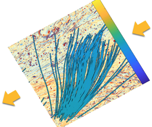
Occurrences strongly reduce for finite directional spread (Slunyaev & Shrira Reference Slunyaev and Shrira2023). Here, wave groups are trapped in a jet, but nonlinear wave interactions are neglected. The high-resolution numerical simulations (see figure 6) reveal that even linear wave trains are well trapped in adversarial currents. Freund & Fleischman (Reference Freund and Fleischman2002) observed a similar behaviour for acoustic waves in a three-dimensional turbulent jet. Note that during our simulation, rays cross the domain several times (because of the doubly periodic boundary conditions; see Appendix E for technical details). At the top (resp. bottom) of the jet, the vorticity and thus – at first order – rays curvatures (Dysthe Reference Dysthe2001) are negative (resp. positive). Therefore, rays oscillate around the jet. A toy model can explain this behaviour. Following the multiscale stochastic approach (4.3)–(4.6), wave scattering is also taken into account.

Figure 6. Rays facing a high-resolution ($512\times 512$) deterministic 2-D Euler jet current – coloured by the corresponding wave amplitude $h(t)=\sqrt {\omega _0(k(t))\,N(t=0)}$ (right-hand side colour bars) – computed by forward advection and superimposed on the current vorticity $\omega = \boldsymbol {\nabla }^{\bot } \boldsymbol {\cdot } \boldsymbol {v}$ (top colour bars).

For very-coarse-grained ($4\times 4$) current $\bar {\boldsymbol {v}}$, oscillation remains, but most of the scattering vanishes, as illustrated by figure 7. Moreover, the curvature of the jet creates artificial wave focusing at $t=8$ and $10$ days. Introducing a time-uncorrelated model (3.11) corrects the resolution issue in figure 8. Figure 9 plots the current ADSD. The current is strong ($\|\boldsymbol {v}\|\approx 1.4$ m s$^{-1}$), and the usual fast wave approximation cannot be applied (${\|\boldsymbol {v}\|}/{v_g^0 } \approx 1.2\times 10^{-1}$). However, the proposed modified fast wave model is valid, even at the very coarse $4\times 4$ resolution.

Figure 7. Rays facing a low-resolution ($4\times 4$) deterministic 2-D Euler jet current – coloured by the corresponding wave amplitude $h(t)=\sqrt {\omega _0(k(t))\,N(t=0)}$ (right-hand side colour bars) – computed by forward advection and superimposed on the current vorticity $\omega = \boldsymbol {\nabla }^{\bot } \boldsymbol {\cdot } \boldsymbol {v}$ (top colour bars).

Figure 8. Rays facing a low-resolution ($4\times 4$) deterministic 2-D Euler jet current plus (one realization of) the time-uncorrelated stochastic model – coloured by the corresponding wave amplitude $h(t)=\sqrt {\omega _0(k(t))\,N(t=0)}$ (right-hand side colour bars) – computed by forward advection and superimposed on the low-resolution current vorticity $\bar {\omega } = \boldsymbol {\nabla }^{\bot } \boldsymbol {\cdot } \bar {\boldsymbol {v}}$ (top colour bars).

Figure 9. The ADSD (m$^2$ s$^{-1}$/(rad m$^{-1}$)) of the resolved high-resolution jet velocity in red, low-resolution jet velocity in blue, and modelled stochastic velocity in green. The theoretical spectrum slope $- 3$ (black solid line) is imposed, consistent with homogeneous 2-D Euler dynamics. The residual ADSD (green line) is set to extrapolate that power law at small scales.

Indeed, 2-D Euler spectra are steeper than for SQG dynamics, and the length scale ratio is already significant at this resolution, ${l_{v'}}/{l_{v}} = 0.14$, and the derived time-decorrelation ratio is small: $\epsilon = ({l_{v'}}/{l_{v}}) ({\|\boldsymbol {v}\|}/{v_g^0}) = 1.6 \times 10^{-2}$.

Furthermore, by approximating the under-resolved current $\bar {v}$, an analytic stochastic solution can be obtained for a ray travelling against the current. The large-scale pattern of the jet takes a quadratic form

(5.3a,b)\begin{equation} \bar{u} \approx \bar{U}_0 - \frac 12\,\bar{\beta} \left(y-\frac{L_y}{2}\right)^2 \quad \textrm{and} \quad \bar{v} \approx 0,\quad \textrm{with}\ \bar{U}_0,\bar{\beta} <0. \end{equation}

Note that the toy model (5.3a,b) simply considers a straight jet, neglecting its curvature. For weak subgrid currents and a ray $(x_r,y_r'+{L_y}/{2},k,\theta _k)$, propagating mainly to the right, $\theta _k$ is small and the simplified ray equation (4.4) determines the group position with respect to the jet $y_r'$:

(5.4)\begin{equation} \frac{{\mathrm{d}} }{{\mathrm{d}} t} y_r'\approx v_g^0 \sin ( \theta_k) = v_g^0 \theta_k+ O(\theta_k^2). \end{equation}

For frozen turbulence, the wavenumber and hence $v_g^0$ will not vary significantly. The other ray equation (4.3) localizes the group along the jet, $x_r \approx x_r(0) + (v_g^0-\bar {u})t$, dropping the $O(\theta _k^2)$ from now on. Moreover, $\tilde {\boldsymbol {k}}^\bot \boldsymbol {\cdot } \boldsymbol {\nabla } \bar {\boldsymbol {v}}^{{\rm T}} \tilde {\boldsymbol {k}} \approx -\partial _y \bar {u}$, and the dynamics of wavevector angle (4.6) simplifies to a stochastic oscillator equation:

(5.5)\begin{equation} \frac{{\mathrm{d}}^2 }{{\mathrm{d}} t^2} y_r'= v_g^0\, \frac{{\mathrm{d}} }{{\mathrm{d}} t} {\theta}_{k}=s-\partial_y (v_g^0 \bar{u}) + v_g^0 \sqrt{3 \gamma_0}\,\dot{B}_t^{(4)}={-} \bar{\omega}_r^2 y_r'+ v_g^0 \sqrt{3 \gamma_0}\,\dot{B}_t^{(4)}, \end{equation}

with $\bar {\omega }_r = \sqrt {|v_g^0 \bar {\beta }|}$. Here, $v_g^0 \bar {u}$ plays the role of a potential, trapping the rays in the jet vicinity, whereas the noise accounts for wave scattering. The solution of this linear equation is known (e.g. Resseguier et al. (Reference Resseguier, Mémin and Chapron2017a), (51)–(55)):

(5.6)\begin{align} y_r (t) = \underbrace{\frac{L_y}{2} + y_r'(0) \cos(\bar{\omega}_rt) + \frac{v_g^0}{\bar{\omega}_r}\,\theta_k(0)\sin(\bar{\omega}_rt)}_{=\,\mathbb{E} (y_r(t) )} +\underbrace{Y_{\gamma_0} \sqrt{ \bar{\omega}_r} \int_{0}^t \sin(\bar{\omega}_r(t-r))\, {\mathrm{d}} B_r^{(4)}}_{=\,y_r''(t)}, \end{align}

with $Y_{\gamma _0} = v_g^0\sqrt {{ 3 \gamma _0}/{\bar {\omega }_r^3} }$. The wavevector angle solution is similar. The solution ensemble mean $\mathbb {E} y_r$ is a simple coherent deterministic oscillator. This mean solution describes well the interaction between the group and the under-resolved current from figure 7. From the coarse-scale vorticity shear plotted in figure 10 in the vicinity of the jet, we can estimate $\bar {\beta } = - 2.7 \times 10^{-11}$ m$^{-1}$ s$^{-1}$. It yields an oscillation frequency $\bar {\omega }_r = 1.3 \times 10^{-5}$ rad s$^{-1}$, i.e. period $2{\rm \pi} /\bar {\omega }_r = 5.7$ days, in agreement with the ray tracing simulations. Note that the high-resolution vorticity shear in figure 10(a) does not suggest any relevant values to explain the ray oscillations. Only the proposed multiscale current decomposition provides a quantitative explanation for these oscillations, and by extension for trapping rays inside the jet. Added to the mean solution, the random parts $y_r''(t)$ are continuous summations of zero-mean incoherent wave fluctuations. At each time $r$, the additive random forcing introduces an oscillation. But the influence of the past excitations is weighed by a sine wave due to the phase change. The group position and wavevector angle are Gaussian random variables (as linear combinations of independent Gaussian variables). Therefore, their finite-dimensional law (i.e. the multi-time probability density function) is entirely defined by their mean and covariance functions. Specifically,

(5.7)\begin{align} \mathbb{E} (y_r''(t)\,y_r''(t+\tau))=\tfrac{1}{4} Y_{\gamma_0}^2 (\cos(\bar{\omega}_r \tau )\,(2 \bar{\omega}_r t - \sin( 2 \bar{\omega}_r t)) +\sin(\bar{\omega}_r \tau )\,(1 - \cos( 2 \bar{\omega}_r t))). \end{align}

In particular, the variance of the vertical positions reads $\sigma _y^2 (t) =\frac {1}{4} Y_{\gamma _0}^2 (2 \bar {\omega }_r t - \sin ( 2 \bar {\omega }_r t))$. At $t= 2{\rm \pi} / \bar {\omega }_r$, the group has oscillated once around the jet, and the maximal position extension reaches $\pm 2\sigma _y = \pm 2\sqrt {{\rm \pi} }\,Y_{\gamma _0} = \pm 42$ km, well confirmed by ray simulations. In contrast, usual fast wave models (e.g. Smit & Janssen Reference Smit and Janssen2019) do not consider the interplay between smooth and rough currents, and hence solely predict a classical scattering with a much faster vertical location spreading: $\pm 2 \sigma _y = \pm 2 \sqrt {(2 {\rm \pi})^3/3}\,Y_{\gamma _0} = \pm 217$ km. For large time, our multiscale approach predicts a scaling in $t$, much slower than the usual scattering $t^3$ scaling.

Figure 10. Vorticity shear $\partial ^2_y u$ of the deterministic 2-D Euler jet current at (a) high-resolution ($512\times 512$) and (b) low-resolution ($4\times 4$), and (c) the corresponding swell system period $2{\rm \pi} /\bar {\omega }_r$. Far from the jet (${\pm }200$ km away), the vorticity shear becomes zero or even positive, so periods larger than $10$ days are cropped.

From the group vertical location and wavevector angle, we can also solve (4.5) analytically to estimate the group wavenumber variations. For small wavevector angles, $-\int _0^t \bar {\sigma } \sin (\zeta ) \,{\rm d} t' \approx 2\int _0^t \bar {\omega } \theta _k \,{\rm d} t' = 2 \bar {\beta }\int _0^t y_r'\theta _k \,{\rm d} t'$, and (4.9) together with the analytic solutions for $y_r'$ and $\theta _k$ give a closed stochastic expression for the group wavenumber. Thus the wavenumber factor $\exp (2 \bar {\beta }\int _0^t y_r'\theta _k \,{\rm d} t')$ oscillates at frequency $2\bar {\omega }_r$, and the oscillations modulate the wave amplitude: $h=\sqrt {E}=\sqrt {\omega _0 N} = \mathrm {constant}\times k^{1/4}$. The modulations are associated with wave–current energy exchanges (Boury et al. Reference Boury, Bühler and Shatah2023), visible in the coloured rays of figures 6, 7 and 8 when the groups enter and exit the jet.

Finally, the conditional ray distribution $p(\boldsymbol {x},\boldsymbol {k} \,|\, \boldsymbol {x}_r^0,\boldsymbol {k}^0,t)$, the action spectrum mean from (4.10) and the action mean from (4.11) can all be derived. For a system initially localized in $(0,{L_y}/{2})$ with action $A^0$, wavenumber $k^0$ and a $\sigma _{\delta \theta _k}^0$-width Gaussian angular spreading, propagating to the right, the action mean reads

(5.8)\begin{equation} \mathbb{E} A(x,y,t)= A^0\delta(x - (v_g^0(k^0)-\bar{u}(y))t)\, \mathcal{N}\left(y-\left.\frac{L_y}{2}\right|\tilde{\sigma}_y^2(t)\right), \end{equation}

with $\mathcal {N} (\cdot \,|\, \tilde {\sigma }_y^2(t))$ a Gaussian function with variance $\tilde {\sigma }_y^2(t) = \sigma _y^2(t) + (({v_g^0}/{\bar {\omega }_r}) \sin (\bar {\omega }_r t) \sigma _{\delta \theta _k}^0)^2$. The action is advected in the horizontal direction, and slowly diffuses along the vertical direction.