


1. Introduction
Small-scale air vehicles are used in a range of operations including transportation (Cai, Dias & Seneviratne Reference Cai, Dias and Seneviratne2014), rescue (Mishra et al. Reference Mishra, Garg, Narang and Mishra2020), agriculture (Zhang & Kovacs Reference Zhang and Kovacs2012) and broadcasting (Holton, Lawson & Love Reference Holton, Lawson and Love2015). Although such small-scale aircraft typically fly in calm air, they are now being tasked to navigate in challenging environments such as urban canyons, mountainous areas and turbulent wakes created by ships. As the occurrence of these extreme scenarios has increased due to climate change, reliable control strategies are critical to achieving stable flight in violent atmospheric disturbances (Jones, Cetiner & Smith Reference Jones, Cetiner and Smith2022; Mohamed et al. Reference Mohamed, Marino, Watkins, Jaworski and Jones2023). In response, this study presents a data-driven flow control approach for a wing experiencing extreme levels of vortical gusts.
In violently adverse airspace, small-scale air vehicles encounter various forms of vortex disturbance characterized by a number of parameters including its vortex strength, size and orientation (Biler et al. Reference Biler, Sedky, Jones, Saritas and Cetiner2021; Stutz, Hrynuk & Bohl Reference Stutz, Hrynuk and Bohl2023). In studying the vortex gust–airfoil interaction, the gust ratio  $G \equiv u_g/u_\infty$ is a particularly important factor, where $u_g$ is the characteristic gust velocity and $u_\infty$ is the free stream velocity or cruise velocity. Flight condition of $G > 1$ is traditionally avoided, which can occur in urban canyons, mountainous environments and severe atmospheric turbulence (Jones & Cetiner Reference Jones and Cetiner2021; Jones et al. Reference Jones, Cetiner and Smith2022). Large-scale aircraft generally do not encounter conditions of $G > 1$ due to their high cruise velocity. However, such a condition becomes an important concern for small-scale aircraft such as drones because of its low cruise velocity, leading to potentially large $G$.
$G$.
Considering such severe conditions in which the spatiotemporal scales of the baseflow unsteadiness and disturbances reach almost the same level in magnitude, our recent study has examined extremely high levels of aerodynamic disturbances with  $0< G\leq 10$ (Fukami & Taira Reference Fukami and Taira2023). In particular, we refer to aerodynamics with $G>1$ as extreme aerodynamics due to the presence of violently strong gusts.
Previous studies of vortex gust–airfoil interactions have mainly focused on scenarios with  $G \leq 1$. For example, Qian, Wang & Gursul (Reference Qian, Wang and Gursul2023) experimentally investigated vortex gust–airfoil interaction under $G \leq 0.5$. They examined the effect of various parameters such as gust ratio, angle of attack and sweep angle of the wing on vortical flows and aerodynamic forces through particle image velocimetry (PIV) measurements. Herrmann et al. (Reference Herrmann, Brunton, Pohl and Semaan2022) considered gust mitigation of flows around a DLR-F15 airfoil under vortex gusts with $G \leq 0.1$. With trailing-edge flaps and a combined proportional-integral feedback/model-based feedforward approach, they achieved 64 % reduction in the lift deviation during quasirandom gust encounters. For conditions of $G \leq 0.71$, Sedky et al. (Reference Sedky, Gementzopoulos, Lagor and Jones2023) has recently developed a closed-loop pitch control strategy to mitigate lift fluctuation for transverse gust encounters.
Our recently proposed data-driven technique called a nonlinear lift-augmented autoencoder uncovers the low-dimensional dynamics of vortical flows experiencing extreme levels of vortex disturbances over a wide parameter space (Fukami & Taira Reference Fukami and Taira2023). We have found that time-varying vortical flow fields spanning the large parameter space can be compressed to only three variables using nonlinear machine learning. In the latent space composed of the three variables, the dynamical trajectories converge to a certain structure, forming the low-dimensional inertial manifold that captures the influence of extreme vortex disturbance on the baseline flow dynamics.
The complex dynamics of vortex–airfoil interactions are driven not only by the gust ratio but also by other factors such as the Reynolds number, wing geometry, disturbance size and orientation. Since different combinations of these parameters create diverse patterns of vortex–airfoil interactions, covering infinitely different scenarios with numerical and experimental studies by naïve parameter sweeps is impractical. This calls for a smart way to sample and extract the fundamental nonlinear dynamics. There is also a need to control these violent flows to achieve some form of stable flight.
For achieving real-time control, a reduced-order model is necessary. Linear techniques such as proper orthogonal decomposition (Lumley Reference Lumley1967; Berkooz, Holmes & Lumley Reference Berkooz, Holmes and Lumley1993) and dynamic mode decomposition (Schmid Reference Schmid2010) have been used to extract low-dimensional flow features and dynamics. However, finding a universal low-order representation over a range of flow configurations or patterns is challenging with linear techniques when mode deformation occurs. In such a case, nonlinear machine-learning-based techniques can be helpful (Brenner, Eldredge & Freund Reference Brenner, Eldredge and Freund2019; Brunton, Hemanti & Taira Reference Brunton, Hemanti and Taira2020a; Brunton, Noack & Koumoutsakos Reference Brunton, Noack and Koumoutsakos2020b).
This study considers leveraging the machine-learned low-order manifold for gust mitigation control. However, controlling such violent flows is challenging due to their transient nature. To address this point, we apply phase-amplitude reduction (Shirasaka, Kurebayashi & Nakao Reference Shirasaka, Kurebayashi and Nakao2017; Nakao Reference Nakao2021) to the low-dimensional extreme aerodynamic manifold for the design of a control law. Phase-amplitude reduction is a technique to analyse oscillatory signals or waveforms in a range of nonlinear dynamic problems (Wedgwood et al. Reference Wedgwood, Lin, Thul and Coombes2013; Wilson & Moehlis Reference Wilson and Moehlis2016; Yawata et al. Reference Yawata, Fukami, Taira and Nakao2024). This analysis can model a given complex dynamics with its phase and amplitude. Phase can be thought of as the timing information of a signal, referring to the position of a waveform at a particular point over time relative to a reference point. However, amplitude represents the intensity of the deviation of the waveform from the reference at a specific point in time (Mauroy & Mezić Reference Mauroy and Mezić2018; Kotani et al. Reference Kotani, Ogawa, Shirasaka, Akao, Jimbo and Nakao2020; Mircheski, Zhu & Nakao Reference Mircheski, Zhu and Nakao2023).
A simplified form of the given complex dynamics with a reduction to its phase and amplitude facilitates dynamical modelling and system control (Kurebayashi, Shirasaka & Nakao Reference Kurebayashi, Shirasaka and Nakao2013; Mauroy, Mezić & Moehlis Reference Mauroy, Mezić and Moehlis2013; Nakao Reference Nakao2016; Takeda, Ito & Kitahata Reference Takeda, Ito and Kitahata2023). Phase-reduction analysis has recently been used to characterize and control fluid flows, including the periodic vortex shedding around cylinders (Taira & Nakao Reference Taira and Nakao2018; Iima Reference Iima2019; Khodkar & Taira Reference Khodkar and Taira2020; Khodkar, Klamo & Taira Reference Khodkar, Klamo and Taira2021; Loe et al. Reference Loe, Nakao, Jimbo and Kotani2021, Reference Loe, Zheng, Kotani and Jimbo2023), a flat plate (Iima Reference Iima2021, Reference Iima2024) and airfoil (Asztalos, Dawson & Williams Reference Asztalos, Dawson and Williams2021; Nair et al. Reference Nair, Taira, Brunton and Brunton2021; Kawamura, Godavarthi & Taira Reference Kawamura, Godavarthi and Taira2022; Godavarthi, Kawamura & Taira Reference Godavarthi, Kawamura and Taira2023). Synchronization characteristics to various forms of periodic perturbations in fluid flows can also be examined with phase-reduction analysis, demonstrated with vortex shedding for a circular cylinder (Taira & Nakao Reference Taira and Nakao2018; Khodkar & Taira Reference Khodkar and Taira2020; Khodkar et al. Reference Khodkar, Klamo and Taira2021; Nair et al. Reference Nair, Taira, Brunton and Brunton2021). For laminar-separated airfoil wakes, phase-reduction-based control design has also shown promise not only to reveal responsible flow physics (Kawamura et al. Reference Kawamura, Godavarthi and Taira2022), but also to optimally modify the wake dynamics (Godavarthi et al. Reference Godavarthi, Kawamura and Taira2023).
This study develops a feedforward control strategy to quickly mitigate the impact of an extreme discrete vortex gust by leveraging the phase-amplitude reduction model on the extreme aerodynamic manifold. The overview of this study is presented in figure 1. There is a step-by-step procedure for preparing the optimal control actuation, aiming to quickly modify the flow state.

The present paper is organized as follows. Extreme aerodynamic flow physics and their low-dimensionalization through a machine-learning technique are introduced in § 2. The method used to prepare the optimal control strategy is described in § 3. Results are presented in § 4. Finally, conclusions are offered in § 5.
2. Extreme vortex–airfoil interactions on a low-dimensional manifold
In this study, we consider extreme vortex gust–airfoil interactions that exhibit strong transient and nonlinear dynamics. To control such violent aerodynamic flows, we develop a data-driven strategy using the sparse identification of nonlinear dynamics (SINDy; Brunton, Proctor & Kutz Reference Brunton, Proctor and Kutz2016a) and phase-amplitude reduction analysis (Takata, Kato & Nakao Reference Takata, Kato and Nakao2021) on a low-dimensional manifold, as presented in figure 1. This section first introduces the model problem and discusses the complex transient flow physics of extreme aerodynamics. We then show how complex, high-dimensional vortical flows under extreme aerodynamic conditions can be compactly expressed in the latent space using a nonlinear autoencoder. Sections 2.2 and 2.3 present the current autoencoder formulation and its use for identifying low-dimensional representations of the dynamics (Fukami & Taira Reference Fukami and Taira2023).
2.1. Flow physics: extreme vortex gust–airfoil interaction
As a model problem, we consider an extreme vortex gust–airfoil interaction around an NACA0012 airfoil with angles of attack  $\alpha \in [20,60]^\circ$ at a chord-based Reynolds number of 100. The datasets are produced by fully resolved (direct) numerical simulations (Ham & Iaccarino Reference Ham and Iaccarino2004; Ham, Mattsson & Iaccarino Reference Ham, Mattsson and Iaccarino2006; Fukami & Taira Reference Fukami and Taira2023). The computational domain is set over $(x, y)/c \in [-15, 30] \times [-20, 20]$ with the leading edge of the wing positioned at the origin. Verification and validation have been performed extensively with previous studies (Liu et al. Reference Liu, Li, Zhang, Wang and Liu2012; Kurtulus Reference Kurtulus2015; Di Ilio et al. Reference Di Ilio, Chiappini, Ubertini, Bella and Succi2018; Zhong et al. Reference Zhong, Fukami, An and Taira2023).
Without the presence of a vortex gust, a wake at  $\alpha = 20^\circ$ is steady while wakes at $\alpha \geq 30^\circ$ exhibit unsteady periodic shedding (limit-cycle oscillation). The current high $\alpha$ is motivated to model unsteady operating (base) conditions at the present Reynolds number. For the disturbed wake cases, an extremely strong vortex gust is introduced upstream of a wing at $x_0/c = -2$ and $y_0/c\equiv Y \in [-0.5, 0.5]$, as illustrated in figure 2. A Taylor vortex (Taylor Reference Taylor1918) is used to model the disturbance with a rotational velocity profile of
 \begin{equation} u_{\theta}=u_{\theta, max}{\dfrac{r}{R}}\exp\left[\dfrac{1}{2}\left({1-\dfrac{r^2}{R^2}}\right)\right] , \end{equation}
where  $R$ is the radius at which $u_{\theta }$ reaches its maximum velocity $u_{\theta, max}$. To cover a variety of wake patterns in this study, the vortex gust is created by randomly chosen gust ratio $G \equiv u_{\theta,max}/u_\infty \in [-4,4]$, its size $D \equiv 2R/c \in [0.5, 2]$ and vertical position of the disturbance $Y$ relative to the wing. Note that the range of gust ratio $G$ considered herein is much larger than that traditionally thought of as flyable (Jones et al. Reference Jones, Cetiner and Smith2022).

Figure 2. (a) Velocity profile of the vortex gust. (b) An example vorticity field with a vortex gust. The parameters considered in the present study are also shown. The same colour scale of vorticity field visualization is hereafter used throughout the paper.
Let us exhibit in figure 3 the entire collection of lift responses in the present data with representative vortical field snapshots. Here, the convective time is set to zero when the centre of the vortex arrives at the leading edge of the airfoil. The present dataset includes 150 disturbed flow cases with 30 cases for each angle of attack. Strong vortex gusts induce a large excitation of aerodynamic forces within a very short time with highly nonlinear transient flow dynamics. Furthermore, the flow exhibits a variety of wake patterns depending on the parameter combination of the set-up including the vortex size, strength and initial position. Due to the nonlinear interaction between the vortex gust and a flow around an airfoil, massive flow separation can occur, creating additional vortical structures.

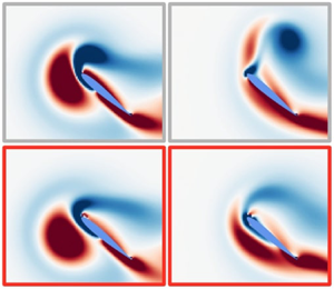
Figure 3. Entire collection of lift history over the parameter space of  $(\alpha,G,D,Y)$ with representative vorticity fields. The vorticity field surrounded by the box (dashed line) is the undisturbed flow for each angle of attack. The dashed and solid lines in the lift curve correspond to the undisturbed case and a representative disturbed case, respectively. The light-blue circles in the parameter spaces correspond to the representative cases chosen for the vorticity field visualizations.
The gust ratio  $G$ is one of the critical parameters that influence the flyability of air vehicles. Here, we examine the effect of $G$ on lift coefficient $C_L$ and vorticity field $\boldsymbol { \omega }$ for cases of $(\alpha,D,Y)=(40^\circ,0.5,0.1)$, as shown in figure 4. We consider $G=\pm 2$ and $\pm 4$ as representative examples. For the positive vortex gusts, lift first increases from the undisturbed state. Once the positive vortex gust impinges on the airfoil, the interaction between the gust and the airfoil wake causes massive separation, contributing to the decrease of the lift over $0< t<1$. In contrast, negative vortex disturbances decrease the lift first with subsequent lift value recovery towards that of the original limit-cycle case in a transient manner. Note that the transient lift generated by these vortices is very large compared with the undisturbed lift level. The fluctuation from the undisturbed lift generally increases as $|G|$ becomes large.

Figure 4. Dependence of lift coefficient  $C_L$ and vorticity field $\boldsymbol { \omega }$ on the gust ratio $G$. The cases for $(\alpha,D,Y)=(40^\circ,0.5,0.1)$ with $G=\pm 2$ and $\pm 4$ are shown. The grey line in the lift response corresponds to the baseline (undisturbed) case.
It is also observed that the difference in  $G$ of the positive gust cases causes the shift in timing for the secondary peak of $C_L$ from $t\approx 0.5$ ( $G=2$) to $0.6$ ( $G=4$). This is because the gust with $G=4$ interacts with the pre-existing negative vorticity on the suction side of the airfoil more strongly than that with $G=2$. As depicted with the vorticity snapshots at $t=0.125$, a stronger interaction with $G=4$ forms a larger negative vortex near the leading edge, compared with the case with $G=2$.
The dependence of the extreme aerodynamic response on the gust size is also investigated, as shown in figure 5. For comparison, we fix the angle of attack, gust ratio and vertical position  $(\alpha, G, Y)=(40^\circ, 3.6, 0.1)$ while varying the gust size $D$ from 0.5 to 2. For all the disturbed cases with different $D$, the lift response exhibits the same trend of first increasing and then decreasing towards the original undisturbed case. The first lift peak appears earlier as the gust size increases since a larger vortex gust reaches the wing earlier, as presented in figure 5. While the gust of $D=0.5$ primarily interacts with the structures near the leading edge, the vortex gust of $D>1$ simultaneously impacts the leading and trailing edge vortices, exhibiting massive separation while newly generating large vortical structures.

Figure 5. Dependence of lift coefficient  $C_L$ and vorticity field $\boldsymbol { \omega }$ on the gust size $D$. The cases for $(\alpha,G,Y)=(40^\circ,3.6,0.1)$ with $D=0.5$, 1, 1.5 and 2 are shown. The grey line in the lift response corresponds to the baseline (undisturbed) case.
The extreme vortex–airfoil interaction dynamics are also affected by the vortex position  $Y$ in addition to gust ratio $G$ and gust size $D$. This causes the difference in the interaction of a vortex gust with the pre-existing vortical structures around a wing. To examine this point, we cover three vertical positions of $Y = (-0.3, 0, 0.3)$ for fixed parameters of $(\alpha, G, D)=(40^\circ, -2.2, 0.5)$, as presented in figure 6. The lift fluctuation for $Y=0.3$ from the undisturbed case is smaller than that for $Y=0$ and $-$0.3 since only the bottom half of the negative vortex gust impinges on the airfoil. By shifting the vortex position downward, a large portion of the gust interacts with the airfoil, producing a large variation of lift force. For $Y=-0.3$, the wing is largely affected by the negative vortex gust at the pressure side, experiencing a larger drop in lift force compared with the other two scenarios.

Figure 6. Dependence of lift coefficient  $C_L$ and vorticity field $\boldsymbol { \omega }$ on the initial vertical position $Y$. The cases for $(\alpha,G,L)=(40^\circ,-2.2,0.5)$ with $Y=-0.3$, 0 and 0.3 are shown. The grey line in the lift response corresponds to the baseline (undisturbed) case.
We further note that the sharp lift responses from extreme vortex gust–airfoil interaction discussed above occur only within two convective times for almost all considered cases. While we easily recognize the difficulty of controlling air vehicles under such a significant variation in the lift force, it also implies that a controller for the present extreme aerodynamic flows needs to quickly modify the flow to attenuate the transient lift responses. This calls for a control technique that can react quickly.
2.2. Lift-augmented nonlinear autoencoder
Analysing the present extreme aerodynamic flows is challenging due to their complexity and nonlinearity. Furthermore, it is challenging to perform a large number of numerical simulations or experiments for studying the vortex–airfoil interaction across a large parameter space with finite resources. Hence, a model that universally captures the fundamental physics of extreme aerodynamics without necessitating expensive simulations and experiments would be beneficial.
In response, we have recently developed a lift-augmented nonlinear autoencoder (Fukami & Taira Reference Fukami and Taira2023) that can compress a collection of extreme aerodynamic vortical flow data across a large parameter space into only a few latent space variables while retaining the original vortex–airfoil interaction. An autoencoder is a neural-network-based model reduction technique (Hinton & Salakhutdinov Reference Hinton and Salakhutdinov2006). As illustrated in figure 7, an autoencoder is composed of an encoder  ${\mathcal {F}}_e$ and a decoder ${\mathcal {F}}_d$ while having the bottleneck where the latent vector ${\boldsymbol { \xi }}$ is positioned. The autoencoder model is generally trained to output the same data as the given input data. In other words, the given high-dimensional input data can be compressed into the latent vector $\boldsymbol { \xi }$ if the autoencoder can successfully decode the original data.

Figure 7. Lift-augmented nonlinear autoencoder (Fukami & Taira Reference Fukami and Taira2023).
In this study, the discrete vorticity field  $\boldsymbol { \omega }$ is compressed through the autoencoder such that
 \begin{equation} {\boldsymbol{ \omega}}\approx{\mathcal{F}}(\boldsymbol{ \omega}) = {\mathcal{F}}_d({\mathcal{F}}_e({\boldsymbol{ \omega}})),\quad {\boldsymbol{ \xi}} = {\mathcal{F}}_e(\boldsymbol{ \omega}),\quad \boldsymbol{\omega} \approx \hat{\boldsymbol{\omega}} = {\mathcal{F}}_d({\boldsymbol{ \xi}}), \end{equation}
where  $\hat {\boldsymbol {\omega }}$ is the decoded (reconstructed) vorticity field. The weights ${\boldsymbol {w}}$ inside a regular autoencoder are optimized by solving the following minimization problem:
 \begin{equation} {\boldsymbol{w}}^* = \underset{{\boldsymbol{w}}}{{\rm argmin}}\, \| {\boldsymbol{\omega}} - \hat{\boldsymbol{\omega}} \|_2=\underset{{\boldsymbol{w}}}{{\rm argmin}}\, \| {\boldsymbol{\omega}} - {\mathcal{F}}({\boldsymbol{\omega}; {\boldsymbol{w}}}) \|_2, \end{equation}
where  ${\boldsymbol {w}}$ is the weights of the autoencoder. By using nonlinear activation functions inside the neural network, an autoencoder can nonlinearly compress high-dimensional data into a low-order subspace, which often achieves higher compression than linear techniques.
While nonlinear autoencoders can be used to compress a variety of vortical flow data (Omata & Shirayama Reference Omata and Shirayama2019; Xu & Duraisamy Reference Xu and Duraisamy2020; Fukami et al. Reference Fukami, Hasegawa, Nakamura, Morimoto and Fukagata2021a; Racca, Doan & Magri Reference Racca, Doan and Magri2023; Smith et al. Reference Smith, Fukami, Sedky, Jones and Taira2024), we have found that the regular formulation expressed in (2.3) does not produce a physically interpretable data distribution in the latent space (Fukami & Taira Reference Fukami and Taira2023). Extracting low-order coordinates associated with dominant aerodynamic features is important in considering not only the interpretation of extreme aerodynamic flows, but also downstream tasks such as developing control strategies. To facilitate the identification of a low-dimensional subspace from the aspect of aerodynamics, the proposed model referred to as a lift-augmented nonlinear autoencoder incorporates the lift coefficient  $C_L(t)$.
In the present formulation, the additional branch network connected with the latent variables  ${\boldsymbol { \xi }}(t)$ (lift decoder, the blue-shaded portion in figure 7) outputs $C_L(t)$. This side network enables ${\boldsymbol {w}}$ to be tuned to capture important vortical structures that are correlated lift due to $\varGamma \propto C_L$, where $\varGamma$ is circulation. This augmentation also helps to capture large transient lift caused by the present extreme vortex–airfoil interactions. The optimization for the weights inside the lift-augmented autoencoder is performed with
 \begin{equation} {\boldsymbol{w}}^* = \underset{{\boldsymbol{w}}}{{\rm argmin}}\,[\|{\boldsymbol{ \omega}}-\hat{\boldsymbol{ \omega}}\|_2 + \beta \|C_L - \hat{C}_L\|_2 ], \end{equation}
where  $\beta$ balances the vorticity field and lift reconstruction loss terms. Here, the weights inside the main part and lift decoder are simultaneously optimized. For the present data-driven study, we use 1200 vorticity snapshots over 10.2 convective times per case. A subdomain of $(x, y)/c \in [-1.4, 4] \times [-1.2, 1.2]$ with spatial grid points $(N_x, N_y) = (240, 120)$ is extracted from the computational domain for the machine-learning analysis. Details on this autoencoder formulation are provided by Fukami & Taira (Reference Fukami and Taira2023).
2.3. Vortex–airfoil interaction on a low-dimensional manifold
With the nonlinear lift-augmented autoencoder, the entire collection of extreme aerodynamic vortical flows spanning over a large parameter space can be compressed into only three latent variables. The latent vectors  ${\boldsymbol { \xi }}(t)$ in the present three-dimensional space are visualized in figure 8(a). Here, undisturbed baseline cases are shown in colour, while grey lines correspond to all the trajectories mapped from the disturbed vorticity flow field data. A variety of vortical flows with and without gust disturbances across five different angles of attack are considered. All of the extreme aerodynamic cases reside in the vicinity of the undisturbed base states, forming the cone-type structure. This cone shape is referred to as an inertial manifold to which the long-time dynamics converge (Foias, Manley & Temam Reference Foias, Manley and Temam1988; Temam Reference Temam1989; De Jesús & Graham Reference De Jesús and Graham2023). That is, the undisturbed periodic wake dynamics provide the backbone of the manifold with the extreme aerodynamic trajectories lying in the vicinity of this manifold in the three-dimensional latent space.

Figure 8. Extreme aerodynamic trajectories in (a) the three-dimensional latent space and (b) its two-dimensional view for the undisturbed baseline cases. (c) Undisturbed vorticity fields at  $\theta = {\rm \pi}/4$ and ${\rm \pi}$ for $\alpha \in [30,60]^\circ$. The values inside each snapshot report the level of unsteadiness with $\sigma _{{\boldsymbol {\omega }}} = \|{\boldsymbol {\omega }}(t)-\bar {\boldsymbol {\omega }}\|_2/\|\bar {\boldsymbol {\omega }}\|_2$.
Here, let us detail the latent trajectories of the undisturbed flows. The latent vectors for the undisturbed flows across the angle of attack are aligned along the  ${\xi }_3$ direction. The case of $\alpha = 20^\circ$ is mapped as a single dot while the other baseline cases with unsteady periodic shedding at $\alpha \geq 30^\circ$ exhibit cyclic trajectories. These observations in the latent space correspond to the steady flow at $\alpha = 20^\circ$ and unsteady limit-cycle oscillations at $\alpha \geq 30^\circ$ of vorticity fields.
The two-dimensional (projected) view of the latent space and representative vorticity fields for  $\alpha \in [30, 60]^\circ$ at two different phases $\theta = {\rm \pi}/4$ and ${\rm \pi}$ are respectively shown in figure 8(b,c). The radius of each limit cycle for the undisturbed cases of $\alpha \geq 30^\circ$ increases with the angle of attack. They also correlate to the level of unsteadiness present in the vorticity field which we quantify as $\sigma _{{\boldsymbol {\omega }}} = \|{\boldsymbol {\omega }}(t)-\bar {\boldsymbol {\omega }}\|_2/\|\bar {\boldsymbol {\omega }}\|_2$, where $\bar {\boldsymbol {\omega }}$ is a time-averaged vorticity field. These values are listed in the representative snapshots for $\alpha \in [30, 60]^\circ$ in figure 8(c). As shown, the value of $\sigma _{{\boldsymbol {\omega }}}$ increases with the angle of attack. In other words, the increase of the radius is due to the increase in flow unsteadiness for each angle of attack case. Furthermore, undisturbed vorticity fields at each phase depicted in figure 8(c) present a similar wake shedding pattern across the angle of attack. These observations suggest that the undisturbed wakes can be successfully low-dimensionalized while preserving the phase (timing) and amplitude (fluctuation) in the original high-dimensional space.
Next, let us focus on the latent space trajectories for the disturbed wake flows. All grey trajectories corresponding to extreme aerodynamic flows reside around the undisturbed orbits. To investigate the implication of low-dimensionalized extreme aerodynamic trajectories, we take an example case of  $(G,D,Y) = (-2.8,1.5,0)$ for which a strong, large vortex gust impinges on an airfoil at $\alpha =60^\circ$. The latent variable trajectory and the reconstructed flow fields over time are also shown in figure 9. The value shown in each decoded flow contour reports the spatial $L_2$ reconstruction error norm $\varepsilon = \|{\boldsymbol {\omega }}-\hat {\boldsymbol {\omega }}\|_2/\|{\boldsymbol {\omega }}\|_2$. The vorticity field can be reconstructed well over time from the three variables with only approximately 20 % error. This level of error is reasonable for capturing the coherent structures accurately because the spatial $L_2$ norm is a strict comparative measure (Fukami, Fukagata & Taira Reference Fukami, Fukagata and Taira2019). While this feature of $L_2$ norm is useful for successful training of nonlinear machine-learning models, one can also consider the structural similarity index (SSIM) for assessing rotational and translational similarities of vortical flows (Wang et al. Reference Wang, Bovik, Sheikh and Simoncelli2004; Anantharaman et al. Reference Anantharaman, Feldkamp, Fukami and Taira2023). The error level here is similar across the parameter space. The lift decoder can also provide accurate estimates of lift coefficient $C_L$, corresponding to approximately 1 % $L_2$ error (Fukami & Taira Reference Fukami and Taira2023). This successful reconstruction indicates that the three-dimensional latent variables retain the essence of high-dimensional vortical flows without significant loss of key physics.

Figure 9. Extreme aerodynamic trajectories in the three-dimensional latent space and vortical flow snapshots for  $(\alpha,G,D,Y) = (60^\circ,-2.8,1.5,0)$. The value inside of each decoded snapshot reports the $L_2$ spatial reconstruction error norm.
The extreme aerodynamic trajectories depicted in figure 9 exhibit the influence of strong vortex gusts on the flow. From the points (a) and (b) in figure 9, the latent vector dynamically rises and drops across the vertical direction in the latent space. This is likely because of the approach of negative vortex disturbance to the airfoil, which drastically changes the effective angle of attack  $\alpha _{eff}$ (Anderson Reference Anderson1991; He et al. Reference He, Deparday, Siegel, Henning and Mulleners2020; Sedky, Jones & Lagor Reference Sedky, Jones and Lagor2020). In other words, the present lift-augmented autoencoder finds the relationship between extreme aerodynamic flows and lift force in a low-order manner. While the latent dimension is generally determined by checking the reconstruction performance of autoencoder, we note that the error behaviour of the present flows plateaus even if the latent dimension is increased as the flows are well approximated in the three-dimensional space with phase-amplitude ( $\theta -r$) coordinates and the effective angle of attack.
The present physically interpretable low-dimensional representation of extreme aerodynamic flows is obtained due to the lift-augmented network while a regular autoencoder may not necessarily provide an understandable latent data distribution (Fukami & Taira Reference Fukami and Taira2023). We emphasize that expressing extreme disturbance effects about the undisturbed baseline dynamics is critical in developing flow control strategies because it enables us to identify the desired direction (or control objective) in the low-order coordinates to mitigate the strong impact of extreme vortex gusts.
3. Phase-amplitude reduction and optimal control
With the uncovered latent space representation, we can quantitatively assess the influence of extreme vortex gusts on the dynamics in a low-order manner. In particular, the present nonlinear coordinate transformation suggests that the vortex–airfoil interaction can be analysed through the latent space with phase  ${\theta }$ and amplitude deviation $r$, as illustrated in figure 10. The latent variable captures similar wake structures at the same phase $\theta$ while showing the amplitude difference attributed to the vortex–airfoil interaction, as exhibited in figure 10(b). This observation suggests that control strategies that push the extreme aerodynamic trajectory towards the direction of the undisturbed baseline state in the latent space mitigate the influence of vortex disturbance in the flow field, naturally calling for a swift system modification on phase-amplitude coordinates.

Figure 10. (a) Extreme aerodynamic manifold with phase and amplitude. The aerodynamic trajectory indicated by the markers, coloured by convective time, corresponds to the case of  $(\alpha, G,D,Y) = (40^\circ, 2.8,0.5,-0.3)$. (b) Two-dimensional plane for $\alpha = 40^\circ$. Flow fields at the same phase but different amplitudes chosen from undisturbed and disturbed cases are inserted.
In this study, we analyse and control extreme aerodynamic flows using phase-amplitude modelling with the following three steps:
(i) dynamical modelling in latent space using SINDy (§ 3.1);
(ii) phase-amplitude reduction to assess phase- and amplitude-sensitivity functions (§ 3.2); and
(iii) control of extreme aerodynamic flows with amplitude-constrained optimal waveform for fast synchronization (§ 3.3).
Using these steps, we derive a control law to suppress the large fluctuation of lift force due to the vortex disturbance within a very short time duration. In this section, we introduce the detailed approach used at each step of the present control strategy.
3.1. Sparsity-promoting low-dimensional dynamical modelling
We model the dynamics of the latent vector  ${\boldsymbol { \xi }}$ with a system of ordinary differential equations (ODEs) using sparse identification of nonlinear dynamics (SINDy; Brunton et al. Reference Brunton, Proctor and Kutz2016a). This data-driven technique identifies nonlinear model equations from given time-series data. Let us consider a dynamical system for the latent vector ${\boldsymbol { \xi }}(t)\in \mathbb {R}^3$,
 \begin{equation}
\dot{\boldsymbol{\xi}}(t) = \boldsymbol{F} (
\boldsymbol{\xi}(t) ).
\end{equation}
\begin{equation}
\dot{\boldsymbol{\xi}}(t) = \boldsymbol{F} (
\boldsymbol{\xi}(t) ).
\end{equation}
The temporally discretized data of  $\boldsymbol {\xi }$ are collected to prepare a data matrix $\boldsymbol {\varXi }$,
 \begin{equation}
\boldsymbol{\varXi}=\left(\begin{array}{@{}c@{}}
\boldsymbol{\xi}^T(t_1) \\ \boldsymbol{\xi}^T(t_2) \\
\vdots \\ \boldsymbol{\xi}^T(t_m)
\end{array}\right)=\left(\begin{array}{@{}ccc@{}} \xi_1(t_1) &
\xi_2(t_1) & \xi_3(t_1) \\ \xi_1(t_2) & \xi_2(t_2) &
\xi_3(t_2) \\ \vdots & \vdots & \vdots \\ \xi_1(t_m) &
\xi_2(t_m) & \xi_3(t_m) \\ \end{array}\right) \in
\mathbb{R}^{m \times 3},
\end{equation}
\begin{equation}
\boldsymbol{\varXi}=\left(\begin{array}{@{}c@{}}
\boldsymbol{\xi}^T(t_1) \\ \boldsymbol{\xi}^T(t_2) \\
\vdots \\ \boldsymbol{\xi}^T(t_m)
\end{array}\right)=\left(\begin{array}{@{}ccc@{}} \xi_1(t_1) &
\xi_2(t_1) & \xi_3(t_1) \\ \xi_1(t_2) & \xi_2(t_2) &
\xi_3(t_2) \\ \vdots & \vdots & \vdots \\ \xi_1(t_m) &
\xi_2(t_m) & \xi_3(t_m) \\ \end{array}\right) \in
\mathbb{R}^{m \times 3},
\end{equation}
where  $m$ is the number of snapshots. We also prepare a library matrix $\varPhi (\boldsymbol {\varXi })$ including nonlinear terms of $\boldsymbol {\varXi }$. This study uses sine and cosine functions for the library matrix construction,
 \begin{align} \varPhi(\boldsymbol{\varXi}) &= ( \sin({\boldsymbol{\varXi}}) \quad \sin({\boldsymbol{\varXi}}/2) \quad \sin({\boldsymbol{\varXi}}/4) \quad \sin({2{\boldsymbol{\varXi}}}) \quad \sin({4{\boldsymbol{\varXi}}}) \quad \cdots\nonumber\\ &\qquad \cos({2{\boldsymbol{\varXi}}}) \quad \cos({4{\boldsymbol{\varXi}}})) \in \mathbb{R}^{m \times n_l}, \end{align}
where we include sine and cosine functions of  $\xi _i$, $\xi _i/2$, $\xi _i/4$, $2\xi _i$ and $4\xi _i$, resulting in the number of the library series $n_l$ to be 10. While polynomials constructed by given variables are often considered for the library matrix construction (Brunton et al. Reference Brunton, Proctor and Kutz2016a; Brunton, Proctor & Kutz Reference Brunton, Proctor and Kutz2016b; Kaiser, Kutz & Brunton Reference Kaiser, Kutz and Brunton2018; Li et al. Reference Li, Kaiser, Laima, Li, Brunton and Kutz2019), we have found that a trigonometric function-based library can provide a more accurate solution for the present problem. The SINDy-based modelling accuracy is determined by a set of factors including the dataset, the number of snapshots, the library functions and the optimization method (Fukami et al. Reference Fukami, Murata, Zhang and Fukagata2021c).
With the data matrix  $\boldsymbol {\varXi }$ and the library matrix $\varPhi (\boldsymbol {\varXi })$, the latent dynamics is modelled as a form of ODE by determining the coefficients for each library term. A coefficient matrix $\varPsi$ is obtained by solving the following regression problem:
 \begin{equation} \dot{\boldsymbol{\varXi}}(t)=\varPhi (\boldsymbol{\varXi}) \varPsi, \end{equation}
with
 \begin{equation} \varPsi = (\psi_{\xi_1} \quad \psi_{\xi_2}\quad \psi_{\xi_3}) = \left(\begin{array}{@{}ccc@{}} \psi _{(\xi_1,1)} & \psi_{(\xi_2,1)} & \psi_{(\xi_3,1)} \\ \psi _{(\xi_1,2)} & \psi_{(\xi_2,2)} & \psi_{(\xi_3,2)} \\ \vdots & \vdots & \vdots \\ \psi _{(\xi_1,n_l)} & \psi_{(\xi_2,n_l)} & \psi_{(\xi_3,n_l)} \\ \end{array}\right). \end{equation}
In this study, the adaptive lasso (Zou Reference Zou2006; Fukami et al. Reference Fukami, Murata, Zhang and Fukagata2021c) is used to optimize the coefficient matrix  $\varPsi$. Once we obtain an accurate low-dimensional dynamical model (3.4), the model is then used to perform the phase-amplitude reduction, which provides the optimal timing and location of control actuation to efficiently and quickly modify the dynamics.
3.2. Phase-amplitude reduction analysis
Here, let us introduce phase-amplitude reduction for a periodic, stable limit-cycle oscillator  $\dot {\boldsymbol { \xi }}(t) = {\boldsymbol {F}}({\boldsymbol { \xi }}(t))$ obtained by the SINDy for each angle of attack case. It is assumed that this ODE has a stable limit-cycle solution ${\boldsymbol {\xi }}_0(t) = {\boldsymbol {\xi }}_0(t+T)$, where $T = 2{\rm \pi} /\omega _{\alpha }$ with the natural frequency $\omega _{\alpha }$ of the latent variable ${\boldsymbol { \xi }}$ for the undisturbed baseline case at each angle of attack $\alpha$. The natural frequency in the latent dynamics matches that in the high-dimensional wake dynamics as the encoder is applied to a time series of flow snapshots.
Given the aforementioned ODE system for the undisturbed system at each angle of attack, we define the phase and amplitude variables  $\theta$ and $r$ of the latent system state ${\boldsymbol { \xi }}$, as illustrated in figures 8 and 10,
 \begin{equation} \theta = \varTheta (\boldsymbol{ \xi}), \quad r = R(\boldsymbol{ \xi}), \end{equation}
where  ${\varTheta }({\boldsymbol { \xi }})$ and $R({\boldsymbol { \xi }})$ are the phase and amplitude functions, respectively. Here, the phase and amplitude functions provide a global linearization of the original nonlinear dynamics in the basin of attraction of the limit cycle for each angle of attack. The phase function $\varTheta$ is defined to satisfy the condition that the phase $\theta$ increases with a frequency $\omega _\alpha$ at an angle of attack $\alpha$. Hence, the generalized phase dynamics is described as
 \begin{equation} \dot{\varTheta}({\boldsymbol{ \xi}}) = \langle \boldsymbol{\nabla}{\varTheta}({\boldsymbol{ \xi}}), \dot{\boldsymbol{ \xi}} \rangle = \langle \boldsymbol{\nabla}{\varTheta}({\boldsymbol{ \xi}}), {\boldsymbol{F}}({\boldsymbol{ \xi}}) \rangle = \omega_{\alpha}, \end{equation}
where  $\langle {\boldsymbol {a}},{\boldsymbol {b}}\rangle = \sum _{i=1}^N a_i^*b_i$ is a scalar product.
Similarly, the generalized amplitude dynamics can also be derived with the assumption that  $r$ exponentially decays to zero as ${\dot r}=\lambda r$ of the limit cycle, as presented in figure 10. Here, $\lambda$ denotes the decay rate given by the Floquet exponent, which characterizes the linear stability of ${\boldsymbol {\xi }}_0$. The connections among the natural frequency $\omega _\alpha$, phase sensitivity function $\varTheta$, Floquet exponents and amplitude sensitivity function $R$ ease the evaluation of phase and amplitude functions as discussed later. Although there are generally $n-1$ amplitudes for $n$-dimensional oscillators associated with the Floquet exponents $\lambda _i$, the dominant, slowest-decaying dynamics is sought whose exponent is denoted as $\lambda$ for simplicity (Nakao Reference Nakao2021). Thus, the amplitude function needs to satisfy
 \begin{equation} \dot{R}({\boldsymbol{ \xi}}) = \langle \boldsymbol{\nabla}{R}({\boldsymbol{ \xi}}), \dot{\boldsymbol{ \xi}} \rangle = \langle \boldsymbol{\nabla}{R}({\boldsymbol{ \xi}}), {\boldsymbol{F}}({\boldsymbol{ \xi}}) \rangle = \lambda R({\boldsymbol{\xi}}). \end{equation}
 Now considering an external control input  ${\boldsymbol {f}}(t)$ to the system, the oscillator dynamics is described as
 \begin{equation} \dot{\boldsymbol{ \xi}}(t) = {\boldsymbol{F}}({\boldsymbol{ \xi}}(t)) + {\boldsymbol{f}}(t). \end{equation}
For this perturbed system, the dynamics of phase  $\theta$ and amplitude $r$ satisfy
 $$\begin{gather} \dot{\theta}(t) = \omega_{\alpha} + \langle \boldsymbol{\nabla}\varTheta({\boldsymbol{ \xi}}(t)), {\boldsymbol{f}}(t) \rangle, \end{gather}$$
 $$\begin{gather}\dot{r}(t) = \lambda r(t) + \langle \boldsymbol{\nabla} R ({\boldsymbol{ \xi}}(t)), {\boldsymbol{f}}(t) \rangle. \end{gather}$$
Here, we further assume that the control input  ${\boldsymbol {f}}(t)$ is of ${O}(\epsilon )$ with $0 < \epsilon \ll 1$. These equations can be then approximated by neglecting the terms of order ${O}(\epsilon ^2)$,
 \begin{equation} \dot{\theta} = \omega_{{\boldsymbol{ \alpha}}} + \langle {\boldsymbol{Z}}(\theta),{\boldsymbol{f}}(t) \rangle, \quad {\dot r} = \lambda r + \langle {\boldsymbol{Y}}(\theta),{\boldsymbol{f}}(t) \rangle, \end{equation}
where  ${\boldsymbol {Z}}(\theta )=\boldsymbol {\nabla } \varTheta |_{{\boldsymbol { \xi }}={\boldsymbol {\xi }}_0(\theta )}$ and ${\boldsymbol {Y}}(\theta )=\boldsymbol {\nabla } {R}|_{{\boldsymbol { \xi }}={\boldsymbol {\xi }}_0(\theta )}$ are the phase and amplitude sensitivity functions, respectively, evaluated on the limit cycle for each angle of attack $\alpha$.
The phase sensitivity function  ${\boldsymbol {Z}}(\theta )$ describes the sensitivity of the system phase and the amplitude sensitivity function ${\boldsymbol {Y}}(\theta )$ reveals the sensitivity of the system amplitude about the periodic orbit against external forcing. Although it is generally difficult to measure the phase and amplitude sensitivity functions, they can be obtained by assessing the left Floquet eigenvectors if a dynamical model is explicitly given (Kuramoto Reference Kuramoto1984; Takata et al. Reference Takata, Kato and Nakao2021).
If a low-order model is available through SINDy, we can derive from Floquet theory the phase and amplitude sensitivity functions  ${\boldsymbol {Z}}(\theta )$ and ${\boldsymbol {Y}}(\theta )$, respectively. Here, we introduce the right and left Floquet eigenvectors ${\boldsymbol {U}}_i$, and ${\boldsymbol {V}}_i$ that are the $T$-periodic solutions,
 $$\begin{gather} {\dot{\boldsymbol{U}}_i}(t) = [{\mathcal{J}}({\boldsymbol{ \xi}}_0(t)) - \lambda_i]{\boldsymbol{U}}_i(t), \end{gather}$$
 $$\begin{gather}{\dot{\boldsymbol{V}}_i}(t) ={-}[{\mathcal{J}}({\boldsymbol{ \xi}}_0(t))^{{\dagger}} - \lambda_i^{\dagger}]{\boldsymbol{V}}_i(t) \end{gather}$$
for  $i=0,1,\ldots, N-1$, where the superscript ${\dagger}$ represents the Hermitian conjugate and ${\mathcal {J}}$ is a $T$-periodic Jacobian matrix of $\boldsymbol {F}$ evaluated about ${\boldsymbol { \xi }}={\boldsymbol { \xi }}_0(t)$ (Ermentrout Reference Ermentrout1996; Brown, Moehlis & Holmes Reference Brown, Moehlis and Holmes2004; Shirasaka et al. Reference Shirasaka, Kurebayashi and Nakao2017; Kuramoto & Nakao Reference Kuramoto and Nakao2019). The phase sensitivity function ${\boldsymbol {Z}}(\theta )$ and the dominant amplitude sensitivity function ${\boldsymbol {Y}}(\theta )$ are then respectively expressed as
 \begin{equation} {\boldsymbol{Z}}(\theta) = {\boldsymbol{V}}_0(\theta/\omega_{{\boldsymbol{ \alpha}}}), \quad {\boldsymbol{Y}}(\theta) = {\boldsymbol{V}}_1(\theta/\omega_{{\boldsymbol{ \alpha}}}) \end{equation}
for  $0 \leq \theta < 2{\rm \pi}$. To obtain the phase and amplitude sensitivity functions ${\boldsymbol {Z}}(\theta )$ and ${\boldsymbol {Y}}(\theta )$, we first solve the ODE in the forward direction (i.e. the direct problem). The adjoint equation is then solved once the Jacobian at each phase for the time period is available so that ${\boldsymbol {U}}_1$ and ${\boldsymbol {V}}_1$ can be calculated (Takata et al. Reference Takata, Kato and Nakao2021).
3.3. Optimal fast flow control with amplitude constraint
Next, we consider feedforward control based on the phase and amplitude sensitivity functions. As illustrated in figure 10, suppressing the amplitude modulation in the low-order space can lead to the mitigation of the gust impact. Furthermore, since we now have a clear direction in the phase-amplitude space to mitigate the impact of gusts, it is possible to achieve fast synchronization with amplitude penalty such that the latent dynamics quickly returns to the undisturbed baseline dynamics while suppressing amplitude deviations (Harada et al. Reference Harada, Tanaka, Hankins and Kiss2010; Zlotnik et al. Reference Zlotnik, Nagao, Kiss and Li2016; Takata et al. Reference Takata, Kato and Nakao2021). For the vortex–airfoil interaction, synchronization at a higher frequency than the natural frequency with amplitude constraints would provide smaller vortical structures in a wake that are weaker than the undisturbed baseline case (Zhang & Haque Reference Zhang and Haque2022; Godavarthi et al. Reference Godavarthi, Kawamura and Taira2023), thereby swiftly reducing the vortex gust impact in the high-dimensional space. Hence, the objective of the present controller is to quickly attenuate the transient dynamics in the low-dimensional latent space  ${\boldsymbol { \xi }}$ with phase locking. We obtain the actuation pattern to achieve the above objective by leveraging the optimal-synchronization waveform with amplitude suppression (Takata et al. Reference Takata, Kato and Nakao2021).
To begin with, let us introduce the relative phase (phase difference)  $\phi (t) = \theta (t) - \omega _{{\boldsymbol {f}}}t$, where $\omega _{{\boldsymbol {f}}}$ is the forcing signal frequency. Assuming that the the control input ${\boldsymbol {f}}$ is given in the form of ${\boldsymbol {f}}(t) = {\boldsymbol {b}}_{{\boldsymbol { \xi }}}(\omega _{{\boldsymbol {f}}} t)$, the phase dynamics becomes
 \begin{equation} \dot{\theta} = {\omega}_{{\boldsymbol{ \alpha}}} + \langle {\boldsymbol{Z}}(\theta),{\boldsymbol{b}}_{{\boldsymbol{ \xi}}}(\omega_{{\boldsymbol{f}}} t) \rangle. \end{equation}
The dynamics of the relative phase is provided as
 \begin{equation} \dot{\phi}(t) = \Delta \varOmega + \langle {\boldsymbol{Z}}(\phi + \omega_{{\boldsymbol{f}}} t),{\boldsymbol{b}}_{{\boldsymbol{ \xi}}}(\omega_{{\boldsymbol{f}}} t) \rangle, \end{equation}
where  $T_{{\boldsymbol {f}}}$ is a period of the periodic forcing input and $\Delta \varOmega = {\omega }_{\boldsymbol {\alpha}}-\omega _{{\boldsymbol {f}}}$. Since this equation is non-autonomous, we consider deriving an autonomous form by averaging over a period of forcing (Kuramoto Reference Kuramoto1984; Hoppensteadt & Izhikevich Reference Hoppensteadt and Izhikevich1997). The asymptotic behaviour of the relative phase dynamics can be approximated as
 \begin{equation} {\dot\phi}(t) = \Delta \varOmega + \varGamma(\phi), \quad \varGamma(\phi) =\dfrac{1}{T_f}\int_0^{T_{{\boldsymbol{f}}}} \langle {\boldsymbol{Z}}(\phi + \omega_{{\boldsymbol{f}}} \tau),{\boldsymbol{b}}_{{\boldsymbol{ \xi}}}(\omega_{{\boldsymbol{f}}} \tau) \rangle \,{\rm d}\tau, \end{equation}
where  $\varGamma (\phi )$ is called the phase coupling function. Phase locking can be achieved if the relative phase becomes a constant such that $\dot \phi \rightarrow 0$. This phase locking is achieved when $- \max \varGamma (\phi ) < \Delta \varOmega < - \min \varGamma (\phi )$, uncovering the Arnold tongue that captures the condition for synchronization (Shim, Imboden & Mohanty Reference Shim, Imboden and Mohanty2007).
Next, we seek the optimal input to achieve the present control objective. The controller is first asked to synchronize the system to a forcing (target) frequency as quickly as possible. In other words, the rate of convergence of  $\phi$ to a fixed, stable phase-locking point $\phi ^*$ needs to be maximized to satisfy $\dot {\phi ^*} = \Delta \varOmega + \varGamma (\phi ^*) = 0$. Furthermore, we also aim to suppress the excitation from the limit-cycle dynamics in the latent space.
To derive the periodic waveform that can satisfy the above conditions, the following cost function is used to formulate an optimization problem,
 \begin{align} {\mathcal{L}}({\boldsymbol{b}}_{{\boldsymbol{ \xi}}}) &={-} \varGamma^\prime (\phi^*) + \nu \left(P - \dfrac{1}{T_f}\int_0^{T_f} \langle {\boldsymbol{b}}_{{\boldsymbol{ \xi}}}(\omega_f\tau), {\boldsymbol{b}}_{{\boldsymbol{ \xi}}}(\omega_f\tau) \rangle \,{\rm d}\tau\right) \nonumber\\ &\quad + \mu (\Delta \varOmega + \varGamma (\phi^*)) - k \left(\dfrac{1}{T_f}\int_0^{T_f} |\langle {\boldsymbol{Y}} (\phi^*+\omega_{{\boldsymbol{f}}} \tau), {\boldsymbol{b}}_{{\boldsymbol{ \xi}}}(\omega_{{\boldsymbol{f}}} \tau)\rangle|^2 \,{\rm d}\tau\right), \end{align}
where  $\nu$ and $\mu$ are Lagrangian multipliers, and $P$ is a constant satisfying $\sqrt {P} \sim {O}(\omega _{{\boldsymbol { \xi }}}\delta )$. The first term contributes to maximizing the synchronization rate $-\varGamma ^\prime (\phi ^*)$, the second term constrains the energy of actuation and the third term directly corresponds to the rate of convergence of $\phi$. In addition, the fourth term penalizes the excitation of the amplitude variable of the amplitude sensitivity function with the weight $k$.
$k$.
The above optimization problem can be solved using the calculus of variations (Zlotnik et al. Reference Zlotnik, Chen, Kiss, Tanaka and Li2013; Takata et al. Reference Takata, Kato and Nakao2021) once we obtain the phase and amplitude sensitivity functions  ${\boldsymbol {Z}}(\theta )$ and ${\boldsymbol {Y}}(\theta )$, respectively, through Floquet analysis for the latent evolution equation derived by SINDy. We can finally derive the optimal waveform as
 \begin{align} {\boldsymbol{b}}_{{\boldsymbol{ \xi}}}(\omega_{{\boldsymbol{f}}} t) &= \tfrac{1}{2} [ \nu {\boldsymbol{\mathsf{I}}} + k \,Re({\boldsymbol{Y}}(\phi^* + \omega_{{\boldsymbol{f}}} t) {{\boldsymbol{Y}}}^{\dagger} (\phi^* + \omega_{{\boldsymbol{f}}} t)) ]^{{-}1}\nonumber\\ &\quad \times[-{\boldsymbol{Z}}^\prime (\phi^* + \omega_{{\boldsymbol{f}}} t) + \mu {\boldsymbol{Z}}(\phi^* + \omega_{{\boldsymbol{f}}} t)], \end{align}
where  ${\boldsymbol {Z}}^\prime$ is the derivative of phase sensitivity function with respect to phase and ${\boldsymbol{\mathsf{I}}}$ is an identity matrix. The weight value $k$ can be chosen either empirically or through the $L$-curve analysis (Hansen & O'Leary Reference Hansen and O'Leary1993) to balance the terms for fast synchronization and the amplitude constraint (Takata et al. Reference Takata, Kato and Nakao2021).
Because the optimal waveform in (3.18) is derived in the latent space, we need to convert it to forcing in the original physical space. Here, we derive the relationship of the perturbation between the latent and physical spaces,  $\Delta {\boldsymbol { \xi }}$ and $\Delta {\boldsymbol { \omega }}$, respectively, for which we assume that the encoder ${\mathcal {F}}_e$ is continuously differentiable. To find such a perturbation $\Delta {\boldsymbol { \omega }}$ towards a particular direction in the physical space, we consider an input vorticity field ${\boldsymbol { \omega }}(t^*)$ with an arbitrary perturbation in the high-dimensional space $\Delta \tilde {\boldsymbol { \omega }}(t^*)$. The latent vector corresponding to the given vorticity field can be approximated with the Jacobian matrix ${\mathcal {J}}_{{\boldsymbol { \xi }}}(\boldsymbol { \omega })$ of ${\mathcal {F}}_e$ evaluated at time $t^*$ such that
 \begin{align} {\boldsymbol{ \xi}} + \Delta \tilde{\boldsymbol{ \xi}} &= {\mathcal{F}}_e ({\boldsymbol{ \omega}}+\Delta \tilde{\boldsymbol{ \omega}})\nonumber\\ & \simeq {\mathcal{F}}_e({\boldsymbol{ \omega}}) + {\mathcal{J}}_{{\boldsymbol{ \xi}}}(\boldsymbol{ \omega}) \Delta \tilde{\boldsymbol{ \omega}}. \end{align}
For the current three-dimensional latent-vector model, we consider giving three different patterns of perturbation to the physical flow field through  $\Delta \tilde {\boldsymbol { \omega }}_m$ $(m=1,2,3)$. From (3.19), the deviation of the latent vector due to the perturbation in the physical space is expressed as
 \begin{equation} \Delta \tilde{\boldsymbol{ \xi}}_m = {\mathcal{J}}_{{\boldsymbol{ \xi}}}\Delta \tilde{\boldsymbol{ \omega}}_m. \end{equation}
For the unit vectors  ${\boldsymbol {e}}_1$, ${\boldsymbol {e}}_2$ and ${\boldsymbol {e}}_3$ in the latent space, the relationship between the perturbation in each direction of the latent dynamics and the deviations in (3.20) is expressed through a coefficient matrix ${\boldsymbol{\mathsf{H}}} \in \mathbb {R}^{3\times 3}$,
 \begin{align} {\boldsymbol{\mathsf{I}}}& =
({\boldsymbol{e}}_1 \quad {\boldsymbol{e}}_2 \quad
{\boldsymbol{e}}_3) =(\Delta \tilde{\boldsymbol{ \xi}}_1
\quad \Delta \tilde{\boldsymbol{ \xi}}_2 \quad \Delta
\tilde{\boldsymbol{ \xi}}_3) \left(\begin{array}{@{}ccc@{}}
{\mathsf{H}}_{11} & {\mathsf{H}}_{12} & {\mathsf{H}}_{13} \\ {\mathsf{H}}_{21} & {\mathsf{H}}_{22} & {\mathsf{H}}_{23} \\
{\mathsf{H}}_{31} & {\mathsf{H}}_{32} & {\mathsf{H}}_{33} \\ \end{array}\right)\nonumber\\
&= {\boldsymbol{D}}_{{\boldsymbol{ \xi}}} {\boldsymbol{\mathsf{H}}}.
\end{align}
\begin{align} {\boldsymbol{\mathsf{I}}}& =
({\boldsymbol{e}}_1 \quad {\boldsymbol{e}}_2 \quad
{\boldsymbol{e}}_3) =(\Delta \tilde{\boldsymbol{ \xi}}_1
\quad \Delta \tilde{\boldsymbol{ \xi}}_2 \quad \Delta
\tilde{\boldsymbol{ \xi}}_3) \left(\begin{array}{@{}ccc@{}}
{\mathsf{H}}_{11} & {\mathsf{H}}_{12} & {\mathsf{H}}_{13} \\ {\mathsf{H}}_{21} & {\mathsf{H}}_{22} & {\mathsf{H}}_{23} \\
{\mathsf{H}}_{31} & {\mathsf{H}}_{32} & {\mathsf{H}}_{33} \\ \end{array}\right)\nonumber\\
&= {\boldsymbol{D}}_{{\boldsymbol{ \xi}}} {\boldsymbol{\mathsf{H}}}.
\end{align}
Hence, to individually perturb the latent system in the  ${\boldsymbol {e}}_1$, ${\boldsymbol {e}}_2$ and ${\boldsymbol {e}}_3$ directions, the perturbation in the high-dimensional space towards a particular direction $\Delta {\boldsymbol { \omega }}_i$ $(i=1,2,3)$ is derived as
 \begin{equation} \Delta {\boldsymbol{ \omega}}_i = \sum_{j=1}^3 {\mathsf{H}}_{ji} \Delta \tilde{\boldsymbol{ \omega}}_j, \end{equation}
where the coefficient matrix can be determined as  ${\boldsymbol{\mathsf{H}}} = {\boldsymbol {D}}^{-1}_{{\boldsymbol { \xi }}}$.
In the present study, the three different perturbations in the physical space (for (3.20)) are determined by a momentum injection at the leading edge of the airfoil at  $45^\circ$, $90^\circ$ and $135^\circ$ relative to the local tangential direction. The actuation cost with the steady momentum coefficient $c_\mu = (\rho u_{jet}^2 \sigma )/(0.5 \rho u_\infty ^2 c)$, where $u_{jet}$ is the actuation velocity and $\sigma$ is the actuator width, is set to be 0.016. Here, three perturbations in (3.20) are individually derived at each $\theta$ over the periodic dynamics because the linearization in (3.19) is locally valid for small perturbation.
The perturbed flow fields and latent vectors (in (3.19)) and the derived forcing in the high-dimensional space corresponding to a perturbation for each direction in the latent space (in (3.22)) are shown in figure 11. The shift of latent vector shown as red, blue and green circles at each phase in figure 11(a) is quite small due to the small forcing input of  $\Delta \tilde {\boldsymbol { \omega }}$. The magnitude and shape of forcing structures depicted in figure 11(b) vary over the dynamics and across the latent variables. The designed forcing is localized due to small forcing inputs for the three different patterns of $\Delta {\boldsymbol { \omega }}$. In this study, we examine how extreme aerodynamic flows can be controlled by such localized actuation spanning over a very small area with the assistance of optimal waveform analysis within a very short time duration.

Figure 11. Conversion from latent perturbation to forcing in the original space. (a) Examples of perturbed vorticity fields  ${\boldsymbol { \omega }} + \Delta \omega$ and the corresponding latent vectors ${\boldsymbol { \xi }} + \Delta \tilde {\boldsymbol { \xi }}$. The colour used for the points in the latent space corresponds to the flame colour for the vorticity field. (b) Perturbation in the high-dimensional space towards a particular direction $\Delta {\boldsymbol { \omega }}_i$.
The identified relationship of the perturbation in the latent and high-dimensional spaces is also used to verify the phase sensitivity function  ${\boldsymbol {Z}}(\theta )$ which is derived in (3.13) (details to be provided later with figure 13). Here, the designed perturbation ${\boldsymbol {K}}_\omega ({\boldsymbol {x}},t)= \epsilon {\boldsymbol {b}}_{{\boldsymbol { \xi }}}(t)\Delta {\boldsymbol { \omega }}({\boldsymbol {x}},t)$ is added to the right-hand side of the vorticity transport equation as
 \begin{equation} \partial_t {\boldsymbol{ \omega}}({\boldsymbol{x}},t) ={-}{\boldsymbol{u}}\boldsymbol{\cdot} \boldsymbol{\nabla} {\boldsymbol{ \omega}} +{Re}^{{-}1} \nabla^2 {\boldsymbol{ \omega}} + {\boldsymbol{K}}_{{\boldsymbol{ \omega}}}({\boldsymbol{x}},t), \end{equation}
where the designed perturbation in the velocity form  ${\boldsymbol {K}}_{{\boldsymbol {u}}} = \boldsymbol {\nabla } \times {\boldsymbol {K}}_\omega$ is used for performing the present simulations (Kawamura et al. Reference Kawamura, Godavarthi and Taira2022). In the next section, we assess the amount of attenuation that can be achieved for extreme aerodynamic flows with the present localized forcing and the optimal waveform.
4. Results and discussion
Let us present the data-driven and phase-amplitude-inspired modelling and control of extreme aerodynamic flows. We consider strong vortex–airfoil interactions at  $\alpha =40^\circ$ as examples. The validity of a low-dimensional dynamical model identified by SINDy is first considered. Once the phase and amplitude sensitivity functions are evaluated with Floquet analysis of the identified low-order model, we apply the present control strategy to the extreme aerodynamic flows for gust mitigation.
4.1. Identification of low-dimensional latent dynamics
Here, we discuss the SINDy-based low-dimensional latent dynamical modelling. As presented in § 3.1, SINDy requires a data matrix  $\boldsymbol {\varXi }$ and its time derivative $\dot {\boldsymbol {\varXi }}$ to approximate the dynamics through regression. To accurately model the dynamics to measure both the phase and amplitude sensitivity functions, giving only the data of the undisturbed periodic oscillation is insufficient because the identified model does not incorporate dynamics of the limit cycle. In other words, the low-order model needs to learn how the dynamics return to the baseline orbit when giving a perturbation (Yawata et al. Reference Yawata, Fukami, Taira and Nakao2024). For this reason, the present training data for SINDy includes not only the periodic oscillation but also the transient process of weakly disturbed cases with a vortex gust. Examples of training vorticity snapshots and corresponding latent vectors are shown in figure 12(a). To consider the transient process, the latent vector ${\boldsymbol { \xi }}$ and their time derivatives $\dot {\boldsymbol { \xi }}$ corresponding to 20 cases with a parameter combination of $G = (\pm 0.1, \pm 0.3, \pm 0.5, \pm 0.7, \pm 0.9)$, $Y= (-0.3, 0.1)$ and $D=0.5$ are prepared. To accurately learn how the dynamics return to the periodic limit cycle, the snapshots after the vortex disturbance passes over an airfoil are used.

Figure 12. (a) Weakly disturbed transient data used for SINDy training. The latent variables and the initial vorticity snapshot for cases with a positive vortex gust with  $Y=0.1$ are visualized. A zoomed-in view of the latent space is also shown. (b) SINDy-based latent dynamics identification. Unperturbed and perturbed model dynamics at $t=0$ are shown.
To assess if the model learns the vicinity of limit-cycle dynamics, the model is integrated with perturbations added at  $t=0$, as shown in figure 12(b). After the perturbation at $t=0$, the amplitude gradually returns to the original level across all latent vectors. This reflects the given airfoil wake physics in the high-dimensional space in which the effect of perturbation dies out over the convection and the wake dynamics come back to the undisturbed periodic shedding oscillation, which is critical to accurately perform phase-amplitude reduction analysis in a low-order space.
4.2. Phase-amplitude-based modelling of latent dynamics
Given the identified model equation, we can apply the phase-amplitude model reduction to obtain the phase and amplitude sensitivity functions. As expressed in (3.12) and (3.13), these functions can be obtained by assessing the left Floquet eigenvectors. These two functions for the present latent dynamics over  $0\leq \theta < 2{\rm \pi}$ are depicted in figure 13(a,b).

Figure 13. (a) Phase sensitivity function  ${\boldsymbol {Z}}(\theta )$ and (b) amplitude sensitivity function ${\boldsymbol {Y}}(\theta )$ for the latent vector $\boldsymbol { \xi }$. For ${\boldsymbol {Z}}(\theta )$, the analytical result through the Floquet analysis ( $-$, Model) and the verified result with the forcing in (3.22) ( $\circ$, Simulation) are shown.
The phase sensitivity functions in the  $\xi _1$ and $\xi _2$ directions are much greater in magnitude than that for $\xi _3$. This is because the latent variables $\xi _1$ and $\xi _2$, which mainly compose the phase plane as illustrated in figure 10, possess a larger variation over the dynamics compared with $\xi _3$ capturing the effective angle of attack on the present manifold. This indicates that perturbing the system in the $\xi _1$ and $\xi _2$ directions is effective in modifying the dynamics from the aspect of phase delay or advancement.
However, the relative magnitude of the amplitude sensitivity function  ${\boldsymbol {Y}}(\theta )$ for $\xi _3$ is of a similar order to that for the other two variables. This implies that the perturbation in the $\xi _3$ direction can contribute to the amplitude modulation of the latent dynamics. This also agrees with the aerodynamic insight in a high-dimensional space in which pitching the wing (in the $\xi _3$ direction) greatly modifies the fluctuation from the mean state of periodic wake shedding.
While being able to derive the phase and amplitude sensitivity functions, these model-based sensitivity functions can be verified by perturbing the vorticity field in a numerical simulation via the conversion, (3.22), and directly assessing the phase shift over the dynamics. The phase sensitivity functions evaluated in this manner are also plotted with circles in figure 13(a). The verified results with the forcing are in excellent agreement with the model-based phase sensitivity function, indicating that the SINDy-based model successfully captures the asymptotic flow behaviour. Note that the amplitude sensitivity function  ${\boldsymbol {Y}}(\theta )$ is not compared with the one measured in the simulation because it is challenging to directly measure ${\boldsymbol {Y}}(\theta )$ in the high-dimensional system (Nakao Reference Nakao2021).
4.3. Amplitude-constrained fast synchronization control
With the phase and amplitude sensitivity functions in hand, we are ready to derive the optimal fast synchronization waveform through (3.17) and (3.18). In this section, we demonstrate how the present method can mitigate the gust impact within a very short time by adding the forcing shown in figure 11 with the optimal waveform.
Let us first apply the present control to the case of  $(\alpha, G,D,Y)=(40^\circ, 2.8, 0.5, -0.3)$ to examine the applicability for which a strong counter-clockwise vortex impinges on a wing. The lift coefficient in this case is violently affected due to the approach of the extreme vortex gust and shows significant fluctuation over a short time of less than 1 convective time. Our aim is to suppress such a sharp force fluctuation within a short time. We initiate actuation at $t=-1.58$ when a vortex gust appears at the left edge of the domain of the interest.
To quantify the control effect, we consider the percentage change of lift fluctuation,
 \begin{equation} \eta = (\Delta C_{L,ctrl} - \Delta C_{L,noctrl})/\Delta C_{L,noctrl}, \end{equation}
where  $\Delta C_L \equiv \max (C_L) - \min (C_L)$ over $-1.58< t<2$ (during a vortex gust impinges a wing) with the subscripts $({\cdot })_{noctrl}$ and $({\cdot })_{ctrl}$ being uncontrolled and controlled variables, respectively. Hence, a negative $\eta$ corresponds to suppression of the lift fluctuation.
To derive the optimal waveform through (3.18), the ratio between the natural frequency  $\omega _{\alpha }$ and the target frequency $\omega _{{\boldsymbol {f}}}$, $\omega _{{\boldsymbol {f}}}/\omega _{\alpha }$, is set to be 1.5 in this case. The choice of target frequency $\omega _{{\boldsymbol {f}}}$ is motivated to quickly modify a flow state since the actuation with $\omega _{{\boldsymbol {f}}}/\omega _{\alpha }>1$ provides faster flow modification than that with $\omega _{{\boldsymbol {f}}}/\omega _{\alpha }<1$ (Godavarthi et al. Reference Godavarthi, Kawamura and Taira2023). For vortex gust–airfoil interaction, it is anticipated that the impact of the gust can be mitigated quickly by changing the vortex-shedding frequency while suppressing the lift excitation due to the vortex gust. Hereafter, we consider the waveform and forcing derived by the latent variable $\xi _3$ based on our aerodynamic knowledge that the effective angle of attack captured by ${\xi _3}$ strongly relates to the lift coefficient. This study chooses an actuation amplitude of $\epsilon = 0.12$, corresponding to $c_\mu =0.24$, to achieve entrainment for extreme aerodynamic flows while ensuring that the actuated dynamics are under the valid regime of phase-amplitude reduction (Godavarthi et al. Reference Godavarthi, Kawamura and Taira2023).
The optimal waveform for the case of  $(\alpha, G,D,Y)=(40^\circ, 2.8, 0.5, -0.3)$ is shown in figure 14(a). To examine the effect of amplitude penalty constrained via (3.17), we consider three different weights, namely $k=0, 0.5$ and 5. The waveform with amplitude penalty provides a more deformed pattern compared with that with $k=0$ designed for purely fast synchronization only, analogous to the observation with several low-dimensional ODE models by Takata et al. (Reference Takata, Kato and Nakao2021).

Figure 14. Phase-amplitude-based control of an extreme aerodynamic flow of  $(\alpha, G,D,Y)=(40^\circ, 2.8, 0.5, -0.3)$. (a) Optimal waveform ${b}_{\xi }$ with $k=0$, 0.5 and 5. (b) Lift coefficient $C_L$ of the uncontrolled and controlled cases with $k=0$, 0.5 and 5. (c) Vorticity fields and (d) lift force elements of the uncontrolled and controlled cases with $k=0$ and 5.
This wave pattern with amplitude penalty provides enhanced suppression of the transient lift fluctuation. The time series of the lift coefficient for each case is presented in figure 14(b). While the lift coefficient with the waveform with  $k=0$ is more amplified, the actuation with the amplitude-constrained optimal waveform successfully suppresses the lift fluctuation, achieving $\eta = -0.357$. We emphasize that the present optimal flow modification strategy is designed with minimal computational cost since all procedures expressed in § 3 are performed in the three-dimensional latent space.
Let us further examine the control effect with vorticity snapshots, as summarized in figure 14(c). While the actuation at the leading edge already affects the vortical flows at  $t=-0.895$, the effect on the vortex gust is clearly observed at $t=0.125$. For $k=0$, the vortex core is shifted up due to the actuation, resulting in strong interaction with the leading-edge vortex at $t=0.975$. This largely contributes to the amplification of lift response. We note that a vorticity field at $t=3.53$ with $k=0$ presents more distinct rolled-up leading and trailing edge vortices that are observed at a high frequency (Godavarthi et al. Reference Godavarthi, Kawamura and Taira2023). This suggests that the fast synchronization-focused optimal waveform can quickly modify the flow states to be a target frequency.
In contrast, the amplitude-constrained optimal actuation with  $k=5$ shifts the vortex core downward and the vortex gust moves to the pressure side of the airfoil. Because of this modification of the vortex-core trajectory, the strong vortex gust merges with the trailing-edge vortex, as seen at $t=0.975$. The wake behaviour then eventually returns to the baseline natural vortex shedding. In other words, the control strategy developed in a low-order space to suppress the amplitude modulation while quickly modifying the low-order dynamics works well to mitigate the gust impact in the high-dimensional physical space. Similar control performance has been confirmed when choosing $\omega _f>1$ and $k\approx 5$.
To further analyse the aforementioned control effect, we perform the force element analysis (Chang Reference Chang1992) which identifies responsible vortical structures for lift generation. Let us define an auxiliary potential function  $\phi _L$ with the boundary condition $-{\boldsymbol {n}}\boldsymbol {\cdot } \boldsymbol {\nabla } \phi _L = {\boldsymbol {n}}\boldsymbol {\cdot } {\boldsymbol {e}}_y$ on the wing surface. Here, ${\boldsymbol {n}}$ is the unit wall normal vector and ${\boldsymbol {e}}_y$ is the unit vector in the lift direction. By taking the inner product of the Navier–Stokes equations with $\boldsymbol {\nabla } \phi _L$ and performing an integral over the fluid domain, the lift force $F_L$ can be expressed as
 \begin{equation} F_L = \int_{{\mathcal{D}}} {\boldsymbol{ \omega}}\times {\boldsymbol{u}}\boldsymbol{\cdot} \boldsymbol{\nabla} \phi_L \,{\rm d}D + \dfrac{1}{Re}\int_{\partial D} {\boldsymbol{ \omega}}\times {\boldsymbol{n}}\boldsymbol{\cdot} (\boldsymbol{\nabla} \phi_L + {\boldsymbol{e}}_y)\,{\rm d}l, \end{equation}
where the first and second terms correspond to the surface integral and the line integral on the wing surface, respectively. The first term is called the lift element  $L_E ({\boldsymbol {x}},t)$, which has often been used to infer the source of lift generation in vortical flows (Moriche et al. Reference Moriche, Sedky, Jones, Flores and García-Villalba2021; Menon, Kumar & Mittal Reference Menon, Kumar and Mittal2022; Ribeiro et al. Reference Ribeiro, Yeh, Zhang and Taira2022; Zhang, Shah & Bilgen Reference Zhang, Shah and Bilgen2022).
Lift element fields over extreme vortex–airfoil interaction are shown in figure 14(d). For the uncontrolled case, the impingement of the vortex gust at  $t=0.125$ greatly contributes to the large transient lift force. It is also observed that the interaction between the vortex gust and the separated leading edge vortex provides positive contribution to lift, which would be difficult to assess from vorticity fields only.
The mechanism of fluctuation suppression with the present control can be understood with the lift element analysis. As shown, the downward shift of vortex core at  $t=0.125$ significantly reduces the positive contribution to the lift force. In addition, at $t=0.975$, the positive vorticity structure generated due to the merging of the vortex gust and the trailing-edge vortex near the pressure side of the airfoil exhibits a negative effect on the lift force. These suggest that the shift of the vortex gust with the present control can indeed reduce the lift force.
Let us also apply the present control to the case of  $(\alpha, G,D,Y)=(40^\circ, -4, 0.5, 0.1)$ to examine the applicability for which a strong negative vortex impinges on a wing. In contrast to the case with positive vortex gusts, the lift force first drops and then increases. The ratio between the target and natural frequencies is set to be $\omega _{{\boldsymbol {f}}}/\omega _{\alpha }=1.3$. The optimal waveform ${\boldsymbol {b}}_{{\boldsymbol { \xi }}}$, the corresponding lift response and vorticity fields are shown in figure 15(a–c). For $k=0$, the lift fluctuation is rather amplified since the actuation is designed for fast synchronization only. By introducing the amplitude penalty, the lift fluctuation can be greatly suppressed, reporting $\eta = -0.410$.

Figure 15. Phase-amplitude-based control of an extreme aerodynamic flow of  $(\alpha, G,D,Y)=(40^\circ, -4, 0.5, 0.1)$. (a) Optimal waveform ${b}_{\xi }$ with $k=0$, 0.5 and 5. (b) Lift coefficient $C_L$ of the uncontrolled and controlled cases with $k=0$, 0.5 and 5. (c) Vorticity fields and (d) lift force elements of the uncontrolled case and the controlled cases with $k=0$ and 5.
Around  $t=-0.8$, the lift force with the amplitude penalty is increased by the actuation. This leads to the cancellation effect for the first drop of the lift force around $t= -0.3$, thereby contributing to the suppression of lift fluctuation. This can also be evident from the shift up of vortex core occurring around the leading edge in a vorticity field at $t=0.125$. Due to this vortex-core shift, the positive contribution to lift is enhanced at the leading edge, as shown in the lift force element field of figure 15(d). Hence, the positive lift generation here contributes to cancelling the reduction of lift force by a strong vortex gust. These observations suggest the possibility of quick flow modification under extreme aerodynamic conditions with local actuation.
5. Concluding remarks
We presented a data-driven approach to mitigate the impact of vortex gusts for flows around an airfoil. In particular, our consideration lies in the conditions of gust ratio  $G>1$ that are challenging to sustain stable flights, referred to as extreme aerodynamics. The present control strategy was developed in a low-dimensional manifold discovered by a nonlinear autoencoder. Once a collection of extreme aerodynamic data is compressed into a three-dimensional latent space, we modelled the dynamics of the latent variables using a sparsity-promoting regression. The identified dynamics as a form of ODE was used to perform phase-amplitude reduction, providing the phase and amplitude sensitivity functions. These functions reveal the system sensitivity in terms of the phase shift and amplitude modulation against a given force input. To quickly suppress the lift fluctuation of extreme vortex gust–airfoil interaction, the control actuation was derived through the amplitude-constrained optimal waveform analysis with the derived phase and amplitude sensitivity functions. We found that the present control technique suppresses lift fluctuation due to a strong vortex impingement within a very short time for a wide variety of scenarios. Furthermore, the successful impact mitigation with a localized forcing implies the possibility of gust control without necessitating drastic pitching motion of the wing. While additional investigations are needed, the proposed data-driven approach may be able to incorporate synthetic jet or plasma actuator-based active flow control strategies (Greenblatt & Williams Reference Greenblatt and Williams2022).
The present observations suggest the importance of physically tractable data compression and preparation of appropriate coordinates to represent complex aerodynamic fluid flow data. The present data compression approach enabled the use of SINDy to model the high-dimensional dynamics in a low-order manner. Furthermore, the compression reduces computational costs in deriving control techniques compared with conventional phase-based analyses performed in the original high-dimensional space, while the preparation for training data and the model development requires substantial effort. The present coherent low-order expression provides a connection between extreme aerodynamic flows and phase-amplitude reduction, enabling the analysis of seemingly complex fluid flows. While the direct application of the present method to higher-Reynolds-number flows may be challenging, one may be able to consider topology-inspired nonlinear machine-learning-based compression that provides phase-amplitude-based coordinates even for non-periodic flows (Smith et al. Reference Smith, Fukami, Sedky, Jones and Taira2024).
There are some conceivable extensions of the present study. One can consider the use of feedback formulation in designing the optimal control actuation in either the SINDy-based model space (Brunton & Noack Reference Brunton and Noack2015; Nair, Brunton & Taira Reference Nair, Brunton and Taira2018) or waveform construction (Takata et al. Reference Takata, Kato and Nakao2021). This could extend the control bounds of the present formulation for high gust ratio and large vortex gusts. While the present study considered library regression-based dynamical modelling whose explicit forms can often be examined (He & Williams Reference He and Williams2023; Fukami, Goto & Taira Reference Fukami, Goto and Taira2024), other candidates such as neural ODE (Linot, Zeng & Graham Reference Linot, Zeng and Graham2023) and recurrent networks (Srinivasan et al. Reference Srinivasan, Guastoni, Azizpour, Schlatter and Vinuesa2019) can be used for low-order dynamical modelling. The dependence of the control performance on the shape and form given as the control input would also be of interest. In addition, the present formulation can be combined with data-driven sparse reconstruction techniques as demonstrated with decoder-type neural-network-based efforts (Erichson et al. Reference Erichson, Mathelin, Yao, Brunton, Mahoney and Kutz2020; Fukami et al. Reference Fukami, Maulik, Ramachandra, Fukagata and Taira2021b; Fukami, Fukagata & Taira Reference Fukami, Fukagata and Taira2023). Towards real-time analysis that is essential for dealing with significant force deviation in a very short time, estimating low-dimensional extreme aerodynamic latent vectors from pressure sensors would be helpful (Fukami & Taira Reference Fukami and Taira2024). Since the proposed control can be performed in a three-dimensional latent space with minimal cost, the present idea of deriving optimal control actuation in a low-order space may prove useful for real-time stable flight operation of modern small-scale aircraft under extreme aerodynamic conditions.
Acknowledgements
We thank Wataru Kurebayashi, Yuzuru Kato, Luke Smith, Alec Linot and Vedasri Godavarthi for insightful discussions.
Funding
K.T. and K.F. acknowledge the support from the US Air Force Office of Scientific Research (grant number: FA9550-21-1-0178) and the US Department of Defense Vannevar Bush Faculty Fellowship (grant number: N00014-22-1-2798). K.F. acknowledges the support from the UCLA-Amazon Science Hub for Humanity and Artificial Intelligence. H.N. acknowledges the support from JSPS KAKENHI (grant numbers: JP22K11919 and JP22H00516) and JST CREST (grant number: JP-MJCR1913).
Declaration of interests
The authors report no conflict of interest.
Appendix A. Assessments of control performance for various extreme aerodynamic scenarios
The present approach finds the optimal actuation based on phase and amplitude sensitivity functions derived from a SINDy-based low-order dynamical model. However, the actuation pattern is designed in a feedforward manner. Furthermore, phase-amplitude reduction involves some linear assumptions, implying that there may exist cases beyond the linear assumptions being valid. Here, we examine the control performance of the present method for extreme vortex–airfoil interactions with various gust parameters to assess these matters.
The concept of phase-amplitude reduction could be leveraged for extreme aerodynamic cases that are mapped in the vicinity of the baseline limit cycle (similar to the case in figure 10). To quantify the deviation from the undisturbed dynamics, we consider the averaged distance  $\Delta R_{{\boldsymbol { \xi }}}$ in a three-dimensional latent space,
 \begin{equation} \Delta R_{{\boldsymbol{ \xi}}} = (\overline{R_{{\boldsymbol{ \xi}},{dist}}}- \overline{R_{{\boldsymbol{ \xi}},{base}}})/\overline{R_{{\boldsymbol{ \xi}},{base}}}, \end{equation}
where
 \begin{equation} R_{{\boldsymbol{ \xi}},{base}}^2 (t_i) = {\sum_j^3 (\xi_{j,{base}}(t_i) - \overline{\xi_{j,{base}}})^2},\quad R_{{\boldsymbol{ \xi}},{dist}}^2 (t_i) = {\sum_j^3 (\xi_{j,{dist}}(t_i) - \overline{\xi_{j,{base}}})^2}, \end{equation}
with the time-averaging operation  $\overline {({\cdot })}$. Hence, $R_{{\boldsymbol { \xi }}}$ measures the deviation from the baseline orbit in the latent space.
The relationship between the control effect  $\eta$ and the distance $\Delta R_{{\boldsymbol { \xi }}}$ is shown in figure 16(a). The plots are coloured by the size of the vortex disturbance $D$. Here, we set the ratio between the natural and target frequencies to be $\omega _{{\boldsymbol {f}}}/\omega _\alpha =1.5$. There is a clear trend – the smaller $\Delta R_{{\boldsymbol { \xi }}}$, the better control performance (a negative $\eta$). The present control is valid for cases that reside near the undisturbed baseline orbit in the latent space, as the effect of gusts may be considered as forcing through the sensitivity functions. Since the dynamical behaviour of the extreme aerodynamic trajectories on the manifold is generally affected by the vortex size more than the gust ratio (Fukami & Taira Reference Fukami and Taira2023), cases with a smaller gust size can be controlled relatively well.

Figure 16. Assessments of the control bounds for extreme aerodynamic flows. (a) Relationship between the control effect  $\eta$ and the deviation of the latent vector from the undisturbed baseline state $\Delta R_{{\boldsymbol { \xi }}}$ coloured by the vortex gust size $D$ and the absolute gust ratio $|G|$. (b) Time series of lift coefficient $C_L$ for cases (i) $(G,D,Y)=(3.6, 1, 0.1)$ and (ii) $(-1.4, 1.5, 0)$ with uncontrolled snapshots.
There are also cases in which the lift fluctuation can be mitigated even with a large vortex gust. We provide a lift curve for two extreme aerodynamic cases involving a large strong vortex gust with the parameters of (i)  $(G,D,Y)=(3.6, 1, 0.1)$ and (ii) $(-1.4, 1.5, 0)$ in figure 16(b). While the lift response of case (i) does not show significant differences after the actuation due to large $G$ and $D$, case (ii) with a larger gust size of $D=1.5$ achieves $15\,\%$ reduction of the lift fluctuation. We should note that the gust ratio of $G=-1.4$ for case (ii) already belongs to the extreme condition. These observations suggest that the present feedforward control strategy developed in a three-dimensional space may provide a step towards flying under extreme aerodynamic conditions.


 Open access