


1. Introduction
The booming importance of microswimmers, mainly in the biomedical sector and environmental remediation, has fueled the research on both living and synthetic microswimmers surrounded by various challenging real-life environments. In addition to developing an enhanced understanding of common biophysical processes, e.g. swimming of spermatozoa through female oviduct (Guidobaldi et al. Reference Guidobaldi, Jeyaram, Condat, Oviedo, Berdakin, Moshchalkov, Giojalas, Silhanek and Marconi2015; Ishimoto & Gaffney Reference Ishimoto and Gaffney2015) and propagation of bacterial infection (Harkes, Dankert & Feijen Reference Harkes, Dankert and Feijen1992), the potential applications of microswimmers range from lab-on-a-chip devices (Denissenko et al. Reference Denissenko, Kantsler, Smith and Kirkman-Brown2012; Bechinger et al. Reference Bechinger, Di Leonardo, Löwen, Reichhardt, Volpe and Volpe2016), assisted fertilization (Magdanz et al. Reference Magdanz, Medina-Sánchez, Schwarz, Xu, Elgeti and Schmidt2017; Bunea & Taboryski Reference Bunea and Taboryski2020), targeted drug delivery using bio-hybrid microbots (Wang & Gao Reference Wang and Gao2012; Park et al. Reference Park, Zhuang, Yasa and Sitti2017; Li et al. Reference Li, Tang, Cong, Lu, Yang, Chen, Zhang and Wu2022) to water treatment using Chlamydomonus sp. (Escudero et al. Reference Escudero, Hunter, Roberts, Helwig and Pahl2020) and other artificial microswimmers (Poddar, Bandopadhyay & Chakraborty Reference Poddar, Bandopadhyay and Chakraborty2019; Chen et al. Reference Chen2021; Yuan et al. Reference Yuan, Gong, Huang, Zhao, Ying and Wang2022).
Microswimmers often have to swim through complex physiological environments by overcoming the effects of a counterflow, thus preventing their downstream transportation. Conversely, a background flow can assist the entrapment of bacteria near surfaces and facilitate surface attachment, which is an essential step for biofilm formation (Rusconi, Guasto & Stocker Reference Rusconi, Guasto and Stocker2014). The background conditions have also been found to influence the migration of droplets (Poddar et al. Reference Poddar, Mandal, Bandopadhyay and Chakraborty2018, Reference Poddar, Bandopadhyay and Chakraborty2019; Mantripragada & Poddar Reference Mantripragada and Poddar2022). The capability of certain microswimmers to change their orientation in response to velocity gradients is known as rheotaxis (Bretherton & Rothschild Reference Bretherton and Rothschild1961; Miki & Clapham Reference Miki and Clapham2013; Ishimoto & Gaffney Reference Ishimoto and Gaffney2015; Sharan et al. Reference Sharan, Xiao, Mancuso, Uspal and Simmchen2022). A common example of this motion characteristic exists during the fertilization process where sperms have to be navigated through a long distance to reach the female eggs (Roberts Reference Roberts1970; Miki & Clapham Reference Miki and Clapham2013; Kantsler et al. Reference Kantsler, Dunkel, Blayney and Goldstein2014). Positive rheotaxis of motile spermatozoa in a Poiseuille flow was reported by Bretherton & Rothschild (Reference Bretherton and Rothschild1961). Later, Rothschild (Reference Rothschild1963) explained the boundary accumulation of sperms due to the difference of drag forces on the head and tail, similar to a weather vane. Under a similar background flow, Kantsler et al. (Reference Kantsler, Dunkel, Blayney and Goldstein2014) observed that the sperm cells migrate differently for varying flow conditions, e.g. upstream spiraling along the bounding substrates and downstream advection for low and high shear velocities, respectively. These motion attributes were described as a combined effect of shear flow, chirality of flagellar beat and steric interaction with the substrate.
Rheotaxis was also reported in bacteria Bacillus subtilis (Marcos et al. Reference Marcos, Fu, Powers and Stocker2012), Escherichia coli (Kaya & Koser Reference Kaya and Koser2012), and artificial microswimmers (Palacci et al. Reference Palacci, Sacanna, Abramian, Barral, Hanson, Grosberg, Pine and Chaikin2015). Subsequently, the theoretical analysis of Uspal et al. (Reference Uspal, Popescu, Dietrich and Tasinkevych2015) revealed that rheotaxis could also occur for spherical active particles, which do not possess shape asymmetry similar to an elongated micro-organism, such as spermatozoa. They showed that the rheotaxis of spherical microswimmers stems from a mechanism of shear-induced rotation near a hard surface, leading to a constrained motion in the shear plane towards the upstream direction at a steady height and orientation. In contrast, theoretical investigations on a virtual monoflagellate Leishmania mexicana promastigote (Walker et al. Reference Walker, Ishimoto, Wheeler and Gaffney2018) predicted no general stable guided taxis under background shear in the absence of a steric contact force at the wall. However, Ishimoto (Reference Ishimoto2017) showed that the inclusion of wall repulsion results in rheotactic states for disc (two dimensional) squirmers, while the same effect further stabilizes the motion of spherical (three dimensional) squirmers of different types.
Although rheotaxis is possible in bulk fluid (Marcos et al. Reference Marcos, Fu, Powers and Stocker2012; Kumar & Ardekani Reference Kumar and Ardekani2019), various attributes of rheotaxis were found to be greatly influenced in the neighbourhood of a liquid–solid interface (Hill et al. Reference Hill, Kalkanci, McMurry and Koser2007; Kaya & Koser Reference Kaya and Koser2012; Mathijssen et al. Reference Mathijssen, Figueroa-Morales, Junot, Clément, Lindner and Zöttl2019). The microfluidic experiments of Hill et al. (Reference Hill, Kalkanci, McMurry and Koser2007) illustrated that the bacteria at the channel centreline have an enhanced tendency of a cross-stream drift towards the channel walls while orienting towards the upstream direction. An enhanced accumulation of micro-organisms at the walls in a uniform shear and a parabolic flow was also reported through computer simulations Chilukuri, Collins & Underhill (Reference Chilukuri, Collins and Underhill2014). Similarly, the work of Mathijssen et al. (Reference Mathijssen, Figueroa-Morales, Junot, Clément, Lindner and Zöttl2019) provided insights into different rheotaxis regimes near a surface, e.g. upstream shifting of swimming orientation, oscillatory rheotaxis and coexistence of rheotactic migration up or against the vorticity direction of the background flow, and also identified the transitional shear rates. Nevertheless, the near-surface accumulating tendency of microswimmers has also been observed even in a quiescent environment (Li & Tang Reference Li and Tang2009; Tailleur & Cates Reference Tailleur and Cates2009; Li et al. Reference Li, Bensson, Nisimova, Munger, Mahautmr, Tang, Maxey and Brun2011; Elgeti & Gompper Reference Elgeti and Gompper2013; Kantsler et al. Reference Kantsler, Dunkel, Polin and Goldstein2013). In addition, different other intriguing near-surface phenomena, such as bacterial entrapment for biofilm formation (Costerton et al. Reference Costerton, Cheng, Geesey, Ladd, Nickel, Dasgupta and Marrie1987), directional circular motion of cells (Lauga et al. Reference Lauga, DiLuzio, Whitesides and Stone2006; Di Leonardo et al. Reference Di Leonardo, Dell'Arciprete, Angelani and Iebba2011), pairwise dancing of Volvox (Drescher et al. Reference Drescher, Dunkel, Cisneros, Ganguly and Goldstein2011) and tumbling trajectories of bacteria E. coli (Kantsler et al. Reference Kantsler, Dunkel, Polin and Goldstein2013), etc. were reported in the absence of a background flow. On the other hand, a significant volume of theoretical studies (Berke et al. Reference Berke, Turner, Berg and Lauga2008; Shum, Gaffney & Smith Reference Shum, Gaffney and Smith2010; Crowdy Reference Crowdy2011, Reference Crowdy2013; Ishimoto & Gaffney Reference Ishimoto and Gaffney2013; Li & Ardekani Reference Li and Ardekani2014; Poddar, Bandopadhyay & Chakraborty Reference Poddar, Bandopadhyay and Chakraborty2020) has shed light on the crucial role of hydrodynamic interaction with the confining substrates in affecting the biophysical dynamics of microswimmers.
The interfacial properties at the solid–fluid or fluid–fluid interfaces were reported to have a substantial contribution in regulating the motion characteristics of a microswimmer near a confining boundary (Lemelle et al. Reference Lemelle, Palierne, Chatre, Vaillant and Place2013; Lopez & Lauga Reference Lopez and Lauga2014; Hu et al. Reference Hu, Wysocki, Winkler and Gompper2015; Pimponi et al. Reference Pimponi, Chinappi, Gualtieri and Casciola2016). The deviation from the no-slip condition at a boundary leads to modulations in the interfacial friction at the micro- and nano-scale (Chakraborty Reference Chakraborty2008; Das et al. Reference Das, Garg, Campbell, Howse, Sen, Velegol, Golestanian and Ebbens2015; Maduar et al. Reference Maduar, Belyaev, Lobaskin and Vinogradova2015). The said deviation is often quantified by a slip length, which is the fictitious distance below the physical wall where the no-slip condition would apply. While, for the hydrophilic surfaces, the slip length is negligible, the same parameter can be significantly higher for the hydrophobic surfaces (Huang et al. Reference Huang, Sendner, Horinek, Netz and Bocquet2008; Bocquet & Charlaix Reference Bocquet and Charlaix2010). Different physical sources behind high slip length has been proposed in the literature. For instance, the slip length can go upto micrometres when the surface is in contact with a bacterial polymeric solution or due to a coating of monolayers of hydrophobic molecules (Tretheway & Meinhart Reference Tretheway and Meinhart2002, Reference Tretheway and Meinhart2004; Lauga, Brenner & Stone Reference Lauga, Brenner and Stone2007). Also, air bubble entrapment between the asperities of micro- and nano-structured surfaces can be treated as an effective continuous partial slip boundary condition (Choi & Kim Reference Choi and Kim2006; Joseph et al. Reference Joseph, Cottin-Bizonne, Benoit, Ybert, Journet, Tabeling and Bocquet2006; Lee et al. Reference Lee, Choi and Kim2008; Nizkaya et al. Reference Nizkaya, Asmolov, Zhou, Schmid and Vinogradova2015).
In relation to microswimmers, Hu et al. (Reference Hu, Wysocki, Winkler and Gompper2015) predicted a transition of model E. Coli bacteria from circular to snaking trajectories due to alterations in the slip length. Similarly, the experimental observation of reversed circular motion of E. Coli due to added polymeric inclusions were estimated to be an effect of intensified slip (Lemelle et al. Reference Lemelle, Palierne, Chatre, Vaillant and Place2013). Lopez & Lauga (Reference Lopez and Lauga2014) employed a far-field analysis based on a force dipole swimmer incorporating non-zero slip lengths and reported that slip induces an additional rotation towards the wall, leading to attraction of pusher-type microswimmers. Very recently, Poddar et al. (Reference Poddar, Bandopadhyay and Chakraborty2020) provided theoretical insights into the effects of high slip on the near-wall trajectories of different types of spherical micro-organisms. They also unveiled that slip length may be chosen as an effective control mechanism for switching from a scattering trajectory to wall entrapment. In another work, Ketzetzi et al. (Reference Ketzetzi, De Graaf, Doherty and Kraft2020) experimentally found that artificial microswimmers show augmented swimming speeds near a hydrophobic surface. These studies considered a quiescent flow condition only, and the effects of different background flows were never looked into. At the other extreme, the literature on rheotactic migration near confinement is limited to the no-slip condition at the wall. In view of the effects brought in by the hydrodynamic slip, it is anticipated that the coupling of the slip condition with the velocity gradients of an external flow (Loussaief, Pasol & Feuillebois Reference Loussaief, Pasol and Feuillebois2015) may non-trivially alter the conditions of stable swimming states, thereby triggering unexplored attributes of rheotaxis.
In the present work we attempt to address the above shortcomings in the literature by formulating a mathematical model of a shear-driven spherical microswimmer in the vicinity of a slippery plane wall. The Navier slip condition has been employed to track the surface wettability condition at the wall. By incorporating the effects of an arbitrary slip length in a squirmer model, the present study stands apart from the widely employed models with asymptotically small slip lengths (Swan & Khair Reference Swan and Khair2008; Willmott Reference Willmott2008). In addition, using the bispherical coordinate system for obtaining an exact solution of the creeping flow problem, the present model aptly captures the hydrodynamics at any distance from the wall, outside the scope of an image-singularity-based analysis (Lopez & Lauga Reference Lopez and Lauga2014). Furthermore, the effects of the Navier slip condition both on the shear flow and the self-propulsion make the outcome of the study unpredictable beyond a simple linear superposition of the slip effects and the corresponding effects with a no-slip boundary condition (Uspal et al. Reference Uspal, Popescu, Dietrich and Tasinkevych2015). We have further performed a detailed analysis of the quasi-steady dynamics of both puller- and pusher-type microswimmers and investigated the effects of different important dimensionless parameters, e.g. dimensionless slip length, shear rate and the squirmer parameter. We also discuss the effect of steric contact interactions on rheotaxis by employing a repulsive force at the wall. It has been found that beyond a critical shear rate, enhancement of slip length can either create new rheotactic states or destroy them depending on a critical interplay between the slip-induced effects and shear flow.
2. Mathematical formulation
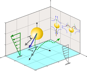
In the present problem, we consider a microswimmer immersed in a background pure shear flow  $\tilde {\boldsymbol {u}}^{(\boldsymbol {ex})}_{\infty }=\dot {\gamma } (\tilde {l}_s+\tilde {z}) \boldsymbol {e}_x$ near a planar wall that obeys the Navier slip condition (Navier Reference Navier1823), as depicted in figure 1. The microswimmer is considered to have a spherical body of radius $a$, and its centre ( $O$) is located at a vertical distance $\tilde {h}$ from the neighbouring slippery wall. The slip length ( $\tilde {l}_s$) can be interpreted as the distance below the plain wall where the extrapolated velocity vanishes. The dimension of the microswimmer is assumed in the range ${O}(10^1\unicode{x2013}10^2) \ \mathrm {\mu } \mathrm {m}$. The orientation of the microswimmer is represented by the director $\hat {\boldsymbol {p}}$, defined as $\hat {\boldsymbol {p}} = p_x \boldsymbol {e}_x + p_y \boldsymbol {e}_y + p_z \boldsymbol {e}_z$, where $p_x = \cos (\theta _p)\cos (\phi _p)$, $p_y = \cos (\theta _p)\sin (\phi _p)$ and $p_z = -\sin (\theta _p)$. Here, we make an assumption that the slip length is uniform along the wall and that the microswimming properties are unaffected by surface texture. Motility of puller- and pusher-type microswimmers are illustrated in the inset, where the blue arrows indicate the mobility direction of the surrounding fluid and green arrows orient towards the local forcing direction of the model swimmer to the fluid if observed from the fixed frame. At this point, we would like to highlight the significance of choosing a three-dimensional (3-D) squirmer model instead of a two-dimensional (2-D) model (Ishimoto & Crowdy Reference Ishimoto and Crowdy2017). The physical phenomenon of upstream swimming or rheotaxis, which is the central theme of the present work, cannot be captured by a 2-D model, while a 3-D model was shown to be successful in this context (Uspal et al. Reference Uspal, Popescu, Dietrich and Tasinkevych2015). It was also shown by Ishimoto & Crowdy (Reference Ishimoto and Crowdy2017) that a 2-D squirmer can only show stable swimming if the Hamiltonian symmetry is broken by perturbations such as weak fluid viscoelasticity (Yazdi, Ardekani & Borhan Reference Yazdi, Ardekani and Borhan2015) or repulsive potential at the wall. Thus, it is essential in the present scenario to adopt a 3-D model of the squirmer to investigate the slip-modulated rheotaxis even in the absence of such external perturbations.

Figure 1. Illustration of a spherical microswimmer in a background pure shear flow  $\tilde {\boldsymbol {u}}^{(\boldsymbol {ex})}_{\infty } = \dot {\gamma } (\tilde {l}_s+\tilde {z}) \boldsymbol {e}_x$ adjacent to a slippery planar wall satisfying the Navier slip condition and having a slip length $\tilde {l}_s$. The microswimmer is of radius $a$, its orientation vector is designated with the vector $\hat {\boldsymbol {p}}$ and the centre (point $O$) is located at a height of $\tilde {h}$ from the wall. Here, $O x' y' z'$ denote the body-fitted reference frame for the microswimmer. The vector $\hat {\boldsymbol {p}}$ makes an angle $\theta _p$ (also known as the pitching angle) with the wall, while $\phi _p$ is its angle with the external flow direction, measured in the plane of the wall. The flow around the model microswimmers in the laboratory frame, for both puller and pusher types, has been schematically shown as an inset.
2.1. Governing equations and boundary conditions
Due to the low Reynolds numbers encountered in flow around microswimmers, the flow field can be described by the Stokes equation (Lauga & Powers Reference Lauga and Powers2009; Michelin & Lauga Reference Michelin and Lauga2014). In addition to this, application of the incompressibility condition leads to the following governing equation for fluid flow:
 \begin{equation} \boldsymbol{\nabla} \boldsymbol{\cdot} \tilde{\boldsymbol{u}}=0 \quad \text{and} \quad -\boldsymbol{\nabla} \tilde{p}+ \mu \nabla ^2 \tilde{\boldsymbol{u}}=0. \end{equation}
Here  $\tilde {\boldsymbol {u}}$ denotes the velocity vector and $\tilde {p}$ is pressure.
The hydrodynamic slip velocity  $\tilde {\boldsymbol {u}}_{||}$ at the slippery plane wall is related to the shear rate at the wall by the Navier slip condition (Navier Reference Navier1823) as
 \begin{equation} \text{at } \tilde{z}= 0, \quad \tilde{\boldsymbol{u}}_{||}= \tilde{l}_{\!_S}\boldsymbol{n}_w\boldsymbol{\cdot}(\boldsymbol{\nabla} \tilde{\boldsymbol{u}}+(\boldsymbol{\nabla} \tilde{\boldsymbol{u}})^{\rm T})(\mathbb{I}-\boldsymbol{n}_w\boldsymbol{n}_w), \end{equation}
where  $\boldsymbol {n}_w$ stands for the unit normal at the plane boundary directed towards the fluid domain and $\mathbb {I}$ represents the identity tensor. The presently developed mathematical model remains applicable for an arbitrary magnitude of the slip length at the plane wall $(\tilde {l}_s)$, in stark contrast to the earlier works with asymptotically small slip lengths (Swan & Khair Reference Swan and Khair2008; Willmott Reference Willmott2008). Moreover, the present model is applicable for a wide range of heights of the microswimmer above the wall, starting from an unbounded domain to the lubrication regime. Hence, the results of the present work cannot be obtained just by considering a linear superposition of the slip-induced effects with those of a no-slip problem. Rather, the slip effects are intrinsically coupled with the hydrodynamic problem, the effects of which can only be visualized through a detailed analysis, as performed subsequently.
The linearity property of the Stokes flow (2.1a,b) and the boundary condition at the microswimmer surface allow us to decompose the full flow problem in two sub-problems ‘sq’ and ‘ex’, to be discussed subsequently. Thus, different flow variables ( $\psi \in [ \tilde {\boldsymbol {u}}, \tilde {\boldsymbol {V}}, \tilde {\boldsymbol {\varOmega }}]$) can be expressed as
 \begin{equation} \psi=\psi^{(sq)}+\psi^{(ex)}, \end{equation}
where  $\tilde {\boldsymbol {V}}$ and $\tilde {\boldsymbol {\varOmega }}$ denote the translational and rotational velocity components of the microswimmer, respectively.
2.1.1. Sub-problem ‘sq’
Diverse swimming appendages, like cilia or flagella, create surface distortions and work behind the motility of microswimmers. We model this swimming action by the ‘squirmer’ model proposed by Lighthill (Reference Lighthill1952) and Blake (Reference Blake1971), and extensively used in literature (Uspal et al. Reference Uspal, Popescu, Dietrich and Tasinkevych2015; Ishimoto Reference Ishimoto2017; Poddar et al. Reference Poddar, Bandopadhyay and Chakraborty2020) related to self-propelling microswimmers. Accordingly, we impose a tangential surface velocity, given by
 \begin{equation} \tilde{\boldsymbol{u}}^{(sq)}_s=\left(\frac{\hat{\boldsymbol{p}}\boldsymbol{\cdot} \boldsymbol{r} }{|\boldsymbol{r}|}\frac{\boldsymbol{r}}{|\boldsymbol{r}|}-\hat{\boldsymbol{p}}\right) \sum_{n=1}^{\infty} \frac{2}{n(n+1)} B_n P'_n\left(\frac{\hat{\boldsymbol{p}} \boldsymbol{\cdot} \boldsymbol{r} }{|\boldsymbol{r}|}\right). \end{equation}
Here,  $\boldsymbol {r}$ denotes the position vector of points on the microswimmer surface with reference to its centre, $B_n$ denotes the amplitude of the $n{{\rm th}}$ squirming mode and $P'_n({\hat {\boldsymbol {p}}\boldsymbol {\cdot } \boldsymbol {r} }/{|\boldsymbol {r}|})$ is the derivative of the Legendre polynomial with respect to the argument ${\hat {\boldsymbol {p}}\boldsymbol {\cdot } \boldsymbol {r} }/{|\boldsymbol {r}|}$. For an unbounded creeping flow, the first squirming mode contributes solely to the propulsion speed, whereas the second mode quantifies the strength of the stresslet exerted by the squirmer (Ishikawa, Simmonds & Pedley Reference Ishikawa, Simmonds and Pedley2006; Li & Ardekani Reference Li and Ardekani2014; Chisholm et al. Reference Chisholm, Legendre, Lauga and Khair2016; Pedley Reference Pedley2016; Pietrzyk et al. Reference Pietrzyk, Nganguia, Datt, Zhu, Elfring and Pak2019). Thus, similar to a host of earlier works (Ishikawa et al. Reference Ishikawa, Simmonds and Pedley2006; Li & Ardekani Reference Li and Ardekani2014; Uspal et al. Reference Uspal, Popescu, Dietrich and Tasinkevych2015; Shaik & Ardekani Reference Shaik and Ardekani2017; Shen, Würger & Lintuvuori Reference Shen, Würger and Lintuvuori2018; Yazdi & Borhan Reference Yazdi and Borhan2017), we retain the first two squirming modes ( $B_1$ and $B_2$) only to capture the essential physics of squirming motion. The ratio of the first two squirming modes $\beta$ arises as an important parameter in the problem, and the parameter helps categorizing the different members of the microswimmer family as puller ( $\beta >0$), pusher ( $\beta <0$) and neutral ( $\beta =0$) types. We further adopt a non-dimensionalization scheme based on reference values chosen for different variables as: length $\sim$ radius of microswimmer $(a)$, velocity $v_{ref} \sim B_1$, time $t_{ref} \sim a/B_1$ and pressure $p_{ref} \sim \mu B_1/a$, and subsequently, remove the symbol ‘ $\tilde {}$’ to represent the corresponding dimensionless quantities. Thus, the boundary condition at the microswimmer surface can be expressed as
 \begin{equation} \text{at} \ r=1, \quad \boldsymbol{u}^{(sq)}=\boldsymbol{V}^{(sq)}+\boldsymbol{\varOmega}^{(sq)} \times \boldsymbol{r} + \boldsymbol{u}^{(sq)}_s. \end{equation}
2.1.2. Sub-problem ‘ex’
In this sub-problem we segregate the effects of a background pure shear flow of the form  $\boldsymbol {u}^{(ex)}_{\infty } = \mathcal {S} (z+l_s) \boldsymbol {e}_x$ on the locomotion of an inert sphere, disregarding the squirming action. Here, $\mathcal {S}$ denotes the dimensionless shear rate of the background flow, defined as $\mathcal {S} = \dot {\gamma } a / v_{ref}$. The sphere undergoes rigid body motion with velocities $\boldsymbol {V}^{(ex)}$ and $\boldsymbol {\varOmega }^{(ex)}$ in the background flow field. In the presence of the sphere, the disturbed velocity can be written as a superposition of the ambient flow $(\boldsymbol {u}^{(ex)}_{\infty } )$ and the perturbation velocity $(\boldsymbol {u}^{(ex)})$ as $\boldsymbol {u}^{(ex)} + \boldsymbol {u}^{(ex)}_{\infty }$. Since the no-slip condition holds true at the particle surface for the disturbed flow, the perturbation velocity satisfies the following boundary condition:
 \begin{equation} \text{at} \ r=1, \quad \boldsymbol{u}^{(ex)}=\boldsymbol{V}^{(ex)}+\boldsymbol{\varOmega}^{(ex)} \times \boldsymbol{r} - \boldsymbol{u}^{(ex)}_{\infty}. \end{equation}
 The unknown velocity components ( $\boldsymbol {V} \ \text {and}\ \boldsymbol {\varOmega }$) are evaluated by considering a neutrally buoyant microswimmer within the flow field, leading to the following force and torque-free conditions:
 \begin{equation} \boldsymbol{F}= \iint\limits_{S_p} {\boldsymbol{\sigma}}\boldsymbol{\cdot} \boldsymbol{n_p}\, {\rm d}S=0 \quad \text{and} \quad \boldsymbol{L}= \iint\limits_{S_p} \boldsymbol{r} \times ({\boldsymbol{\sigma}}\boldsymbol{\cdot} \boldsymbol{n_p})\, {\rm d}S=0. \end{equation}
Now, the thrust force or torque experienced by the microswimmer originates from the squirming action  $(\boldsymbol {F}^{(sq)}_{(Thrust)},\boldsymbol {L}^{(sq)}_{(Thrust)})$ as well as the externally applied flow $(\boldsymbol {F}^{(ex)}_{(Thrust)},\boldsymbol {L}^{(ex)}_{(Thrust)})$. The resultants of these thrusts are further balanced by the hydrodynamic resistance on the rigid sphere $(\boldsymbol {F}_{(Drag)},\boldsymbol {L}_{(Drag)})$. Again exploiting the linearity of the problem, two components of the thrust force can be linearly added, reducing (2.7a,b) to
 \begin{equation} \boldsymbol{F}^{(sq)}_{(Thrust)}+\boldsymbol{F}_{(Thrust)}^{(ex)}+\boldsymbol{F}_{(Drag)}=0 \quad \text{and} \quad \boldsymbol{L}^{(sq)}_{(Thrust)}+\boldsymbol{L}_{(Thrust)}^{(ex)}+\boldsymbol{L}_{(Drag)}=0. \end{equation}
2.2. Solution strategy
In order to solve the above system of governing equations and boundary conditions, together with the force-free constraint, we use eigenfunction expansion of the Stokes flow problem in the bispherical coordinates  $(\xi, \eta, \phi )$ (Happel & Brenner Reference Happel and Brenner1983). In the bispherical system the plane boundary is located at $\xi =0$ and the spherical swimmer surface corresponds to $\xi =\xi _0$ (Behera, Poddar & Chakraborty Reference Behera, Poddar and Chakraborty2023; Poddar Reference Poddar2023). In this solution method the expressions for the velocity components contain a set of unknown coefficients $A_n^m,B_n^m, C_n^m, E^m_n, F_n^m, G_n^m$ and $H^m_n$ (details in Appendix A). To solve for these constants, we employ the different boundary conditions ((2.2a,b), (2.5) and (2.6)), the no penetration condition at the solid surfaces and the incompressibility condition, and apply the orthogonality property of the Legendre polynomials. Due to the decaying nature of these constants, we truncate the infinite series solution of the flow field at large values of $N$ that give an accuracy of $\boldsymbol {O}(10^{-6})$ between successive values of each of the constants considered. The linear algebraic equations to be solved simultaneously for the unknown coefficients have been arranged as a banded matrix of size $7N\times 7N$, to be solved numerically. Higher values of $l_s$ causes convergence issues and an increasingly higher number of terms have to be retained before they are solved numerically. It is to be noted that the simplicity of a no-slip boundary condition at the plane wall allows one to explicitly relate all the other constants in terms of a single constant (O'Neill Reference O'Neill1964) and only a matrix of size $N \times N$ has to be inverted to obtain all the $7N$ desired unknown constants. In contrast, the slip boundary condition complicates the numerical task by demanding a matrix inversion of size $4N\times 4N$. Here, the conversion of an original $7N \times 7N$ system to a smaller matrix size is performed by considering the following compatibility condition (Loussaief et al. Reference Loussaief, Pasol and Feuillebois2015):
 \begin{equation} \frac{\partial u_z}{\partial z} = l_s \frac{\partial^2 u_z}{\partial z^2}. \end{equation}
 The constants  $X_n^m,Y_n^m$ and $Z_n^m$ (A15)–(A16), associated with the boundary conditions on the swimmer surface, take different forms for different sub-problems. They were derived by Shaik & Ardekani (Reference Shaik and Ardekani2017) in relation to the ‘sq’ sub-problem. We derive the corresponding constants for the ‘ex’ sub-problem as
 \begin{align} X_n^1=0, \quad Y_n^1={-}2 \sqrt {2} \, \mathcal{S}\sinh \left( \xi_0 \right) \left( 2n+1 \right) \exp({-( n+1/2 ) \xi_0}) \quad \text{and} \quad Z_n^1=0. \end{align}
The axisymmetry of the truncated squirmer surface velocity model (2.4) confines the orientation vector  $(\hat {\boldsymbol {p}})$ of the body-fitted $x'z'$ plane as shown in figure 1. Consequently, its rotation is fixed along the $y'$ axis. Thus, the squirmer velocities can be written as
 \begin{equation} \boldsymbol{V}^{(sq)}= V^{(sq)}_{z'} \boldsymbol{e}_{z'} + V^{(sq)}_{x'} \boldsymbol{e}_{x'} \quad \text{and} \quad \boldsymbol{\varOmega}^{(sq)}= \varOmega^{(sq)}_{y'} \boldsymbol{e}_{y'}. \end{equation}
In contrast, the symmetry of the pure shear flow imparts a velocity to the inert sphere parallel to the flow direction only, i.e.  $\boldsymbol {V}^{(ex)}= V^{(ex)}_{x} \boldsymbol {e}_{x}$, while the rotational motion of the sphere is triggered along the vorticity direction, i.e. $\boldsymbol {\varOmega }^{(ex)}= \varOmega ^{(ex)}_{y} \boldsymbol {e}_{y}$. Thus, the resultant microswimmer velocities in the fixed frame take the form
 $$\begin{gather} \boldsymbol{V}= (V^{(sq)}_{x'} \cos(\phi_p) + V^{(ex)}_x )\boldsymbol{e}_{x} + V^{(sq)}_{x'} \sin(\phi_p)\boldsymbol{e}_{y} + (V^{(sq)}_{z'} + V^{(ex)}_{z})\boldsymbol{e}_{z}, \end{gather}$$
 $$\begin{gather}\boldsymbol{\varOmega}={-}\varOmega^{(sq)}_{y'}\sin(\phi_p) \, \boldsymbol{e}_{x} + (\varOmega^{(sq)}_{y'}\cos(\phi_p)+\varOmega_{y}^{(ex)}) \boldsymbol{e}_{y}. \end{gather}$$
The details of the ‘squirmer’ thrust components (sub-problem ‘sq’), as well as the hydrodynamic resistance factors (common to both sub-problems ‘sq’ and ‘ex’), can be found in Poddar et al. (Reference Poddar, Bandopadhyay and Chakraborty2020). The thrust components associated with the external flow (sub-problem ‘ex’) have been evaluated by solving the Stokes problem of pure shear flow around a fixed sphere (i.e. only a part of sub-problem ‘ex’), i.e. considering the boundary condition
 \begin{equation} \text{at} \ r=1, \quad \boldsymbol{u} ={-} \boldsymbol{u}^{(ex)}_{\infty}. \end{equation}
The thrust force and torque due to the external flow are thus obtained as
 \begin{equation} F^{(ex)}_{(Thrust,x)}={-}{\sqrt{2}{\rm \pi}}\,\mathcal{S}(l_s+\cosh(\xi_0))\sinh(\xi_0)\sum_{n=0}^{\infty} [G_n^1-H_n^1+n(n+1)(A_n^1-B_n^1)], \end{equation}
 \begin{align} L^{(ex)}_{(Thrust,y)} &={\sqrt{2}{\rm \pi}}\,\mathcal{S}\sinh^2(\xi_0)\sum_{n=0}^{\infty} [\coth(\xi_0)\{n(n+1)(A_n^1-B_n^1)+(G_n^1-H_n^1)\} \nonumber\\ &\quad -2n(n+1)C_n^1 -(2n+1)(G_n^1-H_n^1)]. \end{align}
It is to be noted that the thrust due to the external flow can be alternatively calculated by using the Lorentz reciprocal theorem (LRT) as outlined in Poddar et al. (Reference Poddar, Bandopadhyay and Chakraborty2020) for motion near a slippery plane, thus bypassing the solution to the full Stokes problem. We use LRT only to verify the results obtained by the full solution technique, as presented above.
2.3. Swimming trajectories
The quasi-steady dynamics of the microswimmer (Spagnolie & Lauga Reference Spagnolie and Lauga2012; Uspal et al. Reference Uspal, Popescu, Dietrich and Tasinkevych2015; Mozaffari et al. Reference Mozaffari, Sharifi-Mood, Koplik and Maldarelli2016; Walker et al. Reference Walker, Ishimoto, Wheeler and Gaffney2018) can be fully described by simultaneously determining the location of the microswimmer in space  $\boldsymbol {r} (t)$ along with its preferential orientation with respect to the plane wall, represented by $\hat {\boldsymbol {p}} (t)$. Thus, the trajectories can be obtained by simultaneously solving the following set of coupled ordinary differential equations:
 \begin{equation} \frac{{\rm d}\boldsymbol{r}(t)}{{\rm d}t}=\boldsymbol{V} (\boldsymbol{r}(t),\hat{\boldsymbol{p}}(t))\quad \text{and} \quad \frac{{\rm d}\boldsymbol{\hat{p}(t)}}{{\rm d}t}=\boldsymbol{\varOmega}(\boldsymbol{r}(t),\hat{\boldsymbol{p}}(t)) \times \hat{\boldsymbol{p}}(t) \end{equation}
for a given set of initial conditions  $(\boldsymbol {r}_0,\hat {\boldsymbol {p}}_0)$. The different translational and rotational velocity components at each time instant can be obtained by a combination of their self-propulsion and external flow counterparts, as discussed in (2.12). We neglect the effects of stochastic forces on the microswimmer motion and compute the trajectories considering the deterministic forces only (Shum et al. Reference Shum, Gaffney and Smith2010; Spagnolie & Lauga Reference Spagnolie and Lauga2012; Mozaffari et al. Reference Mozaffari, Sharifi-Mood, Koplik and Maldarelli2016; Poddar, Bandopadhyay & Chakraborty Reference Poddar, Bandopadhyay and Chakraborty2021).
3. Results and discussion
In this section we illustrate the combined interaction of wall slip and a background shear flow in dictating the locomotion characteristics of both puller- and pusher-type microswimmers. The dimensionless analysis presented above can fully describe the rheotactic swimming near a slippery plane using the parameters dimensionless shear rate  $\mathcal {S}$, slip length $l_s$ and squirmer parameter $\beta$; in addition to the positional $(\boldsymbol {r})$ and orientational variables of the microswimmer $(\hat {\boldsymbol {p}})$. In the following subsections we discuss the 3-D trajectories under the influence of different dimensionless parameters involved. Subsequently, we summarize these effects in the form of regime maps and illuminate on the governing physics behind contrasting motion characteristics.
In order to estimate the practical values of the parameter  $\mathcal {S} = \dot {\gamma } a / v_{ref}$, we consider realistic ranges of the dimensional quantities in different microfluidic experiments related to microswimmers (Kantsler et al. Reference Kantsler, Dunkel, Blayney and Goldstein2014; Ohmura et al. Reference Ohmura, Nishigami, Taniguchi, Nonaka, Ishikawa and Ichikawa2021), as stated below: shear rate $\dot {\gamma } = 0.1\ {\rm s}^{-1}$ to $20\ {\rm s}^{-1}$, velocity of a typical microswimmer $v_{ref} = 10 \ \text {to} \ 100 \ \mathrm {\mu } {\rm m}\ {\rm s}^{-1}$ and the length scale of the microswimmer $a = 10 \ \text {to} \ 100 \ \mathrm {\mu } {\rm m}$. Although $\mathcal {S}$ ranges in $\boldsymbol {O}(10^{-2}\unicode{x2013}10^{2})$, a high value of the same parameter amounts to sweeping away of the microswimmer along the external flow. Consequently, the competitive effects of the shear flow and self-propulsion remain obscure. Thus, motivated by the earlier theoretical investigations (Uspal et al. Reference Uspal, Popescu, Dietrich and Tasinkevych2015; Walker et al. Reference Walker, Ishimoto, Wheeler and Gaffney2018), we choose $\mathcal {S}$ between 0 to 1. Similarly, considering previous experimental observations, the dimensionless slip length $(l_{s})$ is varied between 0 and 10 (Zhu & Granick Reference Zhu and Granick2001; Tretheway & Meinhart Reference Tretheway and Meinhart2002; Huang et al. Reference Huang, Sendner, Horinek, Netz and Bocquet2008).
3.1. Swimming states for puller microswimmers
Here, we investigate the modulations in the rheotactic states of puller microswimmers brought in by the near-wall hydrodynamic slip. Consideration of only hydrodynamic forces can resolve the microswimmer dynamics only upto a finite gap with the solid flat surface (Shum et al. Reference Shum, Gaffney and Smith2010; Spagnolie & Lauga Reference Spagnolie and Lauga2012; Uspal et al. Reference Uspal, Popescu, Dietrich and Tasinkevych2015) due to the requirement of infinite computational resources. Thus, the present trajectory simulations based on forces of pure hydrodynamics origin have been performed by considering a minimum distance between the microswimmer surface and the wall as  $\delta = 0.01$. Consequently, any swimming state indicating a downward descend below this gap is considered as a ‘crashing’ or ‘collision’ state (Uspal et al. Reference Uspal, Popescu, Dietrich and Tasinkevych2015). This mathematical treatment is justified since below this small gap, nanoscale interaction forces other than a hydrodynamic origin (Klein, Clapp & Dickinson Reference Klein, Clapp and Dickinson2003) become prominent and are expected to influence the motion characteristics. However, to facilitate a direct comparison of the present results with the previously reported no-slip cases (Uspal et al. Reference Uspal, Popescu, Dietrich and Tasinkevych2015), we have not considered any non-hydrodynamic repulsive force at the plain surface. On the other hand, a microswimmer going beyond a height of $h= 15$ marks its ‘escape’ from the wall, similar to earlier works (Ishimoto & Gaffney Reference Ishimoto and Gaffney2013; Poddar et al. Reference Poddar, Bandopadhyay and Chakraborty2020).
The 3-D trajectories of the microswimmer moving in a background pure shear flow with or without near-wall slippage for different initial orientations ( $\theta _0$) have been compared in figure 2. Figure 2(a) demonstrates that near a no-slip wall the microswimmer swims against the flow with damped amplitude oscillations in the vertical direction and finally shows a sliding motion after reaching an out-of-plane angle $\phi _p=83^{\circ }$, keeping a constant height $h=1.23$ and orientation $\theta _p=27.5^{\circ }$. These motion characteristics have been termed as ‘upstream rheotaxis’ in the literature (Uspal et al. Reference Uspal, Popescu, Dietrich and Tasinkevych2015; Ishimoto Reference Ishimoto2017; Walker et al. Reference Walker, Ishimoto, Wheeler and Gaffney2018).

Figure 2. Trajectories of a puller microswimmer  $(\beta = 7)$ in background pure shear flow ( $\mathcal {S}=0.1$), starting from the same set of initial conditions $x_0=0, y_0=0, h_0=2, \phi _0 = 270^{\circ }$ but different pitch angles, (a,b) $\theta _0=10^{\circ }$ and (c,d) $\theta _0=150^{\circ }$. The effects of the slippery $(l_s=1)$ and no-slip boundary conditions on the trajectories are studied. Red solid trajectories are 3-D representations of motion. Blue and black dashed lines are the projections of the 3-D trajectories on the $xz$ and $yz$ planes, respectively. Arrowheads represent the directions of motion of the microswimmer.
In stark contrast, in the presence of wall slip  $(l_s=1)$, the microswimmer comes in close proximity to the wall and descends below $\delta = 0.01$, which indicates a ‘collision’ state in the absence of an additional contact force (shown in figure 2b). It is worth mentioning that the cutoff distance for trajectory simulations leaves the possibility for the mathematical model to predict more stable swimming states against the flow (rheotaxis) instead of the collision states presented here if the numerical simulations were performed for wall gaps below $\delta =0.01$. Thus, the collision states predicted through a pure hydrodynamic analysis may not be observed if a non-hydrodynamic repulsive interaction at the wall is considered.
However, an altered orientation angle ( $\theta _0=150^{\circ }$) results in an escaping trajectory for the no-slip case, as presented in figure 2(c). Near the boundary, the microswimmer experiences a strong counterclockwise (CCW) reorientation torque due to hydrodynamic interaction with the wall. This enhanced torque has a tendency to rotate the director away from the wall and the vertical velocity switches from $V_z<0$ to $V_z>0$ at a point, resulting in a rapid reorientation of the microswimmer.
The collision states created by the wall slip in figures 2(b) and 2(d) suggest that the said torque is weakened by the slip effects, thus failing to supply the required reorientation for rheotactic sliding or escape. Further comparing the two collision states in the presence of the wall slip, it is found that collision occurs much earlier with  $\theta _0=10^{\circ }$ (at $t_{c}=2.8$) than $\theta _0=150^{\circ }$ (at $t_{c}=12$), despite the director $\hat {p}$ initially tilting more towards the wall in the latter scenario. Here, $t_{c}$ refers to the collision time, which is the duration until the microswimmer descends to $\delta =0.01$ within the flow field. This is due to the contrasting consequences of the slip-induced torque in the two situations. While for $\theta _0={10^{\circ }}$, the said torque assists rotation towards the wall, it favours a director movement away from the wall for $\theta _0={150^{\circ }}$. However in the latter case, this slip-triggered torque is not sufficient for escaping or rheotactic sliding since the cutoff height $\delta =0.01$ has already been encountered.
A comprehensive understanding of the non-trivial motion characteristics due to the diverse plausible combinations of the parameters  $l_s$, $\beta$ and initial conditions demands a large number of individual long-time trajectory simulations in three dimensions, calling for a massive computational time. However, the analysis can be greatly simplified by using the theory of dynamic systems and considering the symmetries in the system. In this regard, we align the plane of microswimmer motion $(x'z')$ along the plane of the background flow $(xz)$, and thus preventing rotation out of the shearing plane. Hence, the pitch angle $\theta _p$ fully parametrizes the angular orientation of the director $\hat {\boldsymbol {p}}$, without loss of generality. As a result, the dynamics of the microswimmer can be described by a plane autonomous system, i.e.
 \begin{equation} \frac{{\rm d}h(t)}{{\rm d}t}=V^{(sq)}_{z'} + V^{(ex)}_{z} \quad \text{and} \quad \frac{{\rm d}\theta_p(t)}{{\rm d}t}=\varOmega^{(sq)}_{y'}+\varOmega_{y}^{(ex)}. \end{equation}
The relevance of the above dimensionally reduced system in predicting the behaviour of the full system was thoroughly examined by Walker et al. (Reference Walker, Ishimoto, Wheeler and Gaffney2018), and long-time simulations of the full system (2.15) were found to be in accordance with the restricted system.
3.1.1. Annihilation of rheotactic states
Here we provide a concise representation of puller dynamics by analysing the phase portraits obtained from (3.1), the results of which are shown in figures 3(a)–3( f). The justification behind the consideration of the phase-plane dynamics instead of analysing all possible out-of-plane dynamics has been discussed in Appendix B. The results corresponding to the no-slip wall in figures 3(a) and 3(d) are in perfect agreement with the work of Uspal et al. (Reference Uspal, Popescu, Dietrich and Tasinkevych2015). As shown in figure 3(a), in a quiescent environment  $(\mathcal {S}=0)$, two stable dynamical attractors (black square markers) appear between $\theta _p=0^{\circ }$ and ${180^{\circ }}$ at mirror symmetric locations about $\theta _p={90^{\circ }}$. These points indicate the final swimming states of the microswimmer as sliding at a steady height and fixed orientation but in opposite directions along the $x$ axis. However, the invariance of the dynamic system along $x$ in the absence of a background flow leads to the same sense of these swimming states, similar to the reported results of Uspal et al. (Reference Uspal, Popescu, Dietrich and Tasinkevych2015). This stable swimming state is a sole consequence of the propulsive torque generated beyond a critical value of $\beta$ (Li & Ardekani Reference Li and Ardekani2014; Poddar et al. Reference Poddar, Bandopadhyay and Chakraborty2020). In addition, two unstable fixed points (red triangles) and a saddle point (denoted with an orange cross) are observed in the same phase portrait. The slip condition at the wall $(l_s>0)$ severely influences the dynamics, as can be found by comparing figures 3(b) and 3(c) with figure 3(a). For a low value of slip length $l_s = 0.36$, the unstable fixed points disappear from the phase portrait and the steady-state height $(h^*)$ corresponding to the attractors comes downward. While this trend of downward shifting fixed points retained for higher slip lengths (e.g. $l_s=1$ in figure 3c), the microswimmer gradually descends below a height $\delta = 0.01$, and finally, collides against it, thus wiping out the attractors from the phase portrait. As a concurrent effect, the unstable fixed points are also suppressed.

Figure 3. Phase space diagrams ( $\theta _p \text {-} h$ plot) for the reduced dynamical system in the $x$–
$x$– $z$ plane for a puller microswimmer $(\beta = 7)$. Absence of external flow presented in (a–c) for $l_s=0$ , $0.36$ and $1$ slip lengths. The dimensional shear rate has been chosen as $\mathcal {S}=0.1$ in (d–f) along with the same environment for the microswimmer. Green circular markers indicate the rheotactic attractor whereas black squares imply the non-rheotactic attractor that is unstable for $\phi \neq 0$. (g) Range of the rheotaxis zone is shown for different slip lengths before annihilation by the plotting vertical distance ( $h^*$) of the rheotactic attractor for different slip lengths. (h) Behaviour of the saddle point (near $\theta ^*>270^{\circ }$) is plotted for different slip lengths $l_s$. The green and red superimposed lines in (d, f), respectively, denote the sample phase space trajectories starting from $h_0=2$ and $\theta _{p,0} =153.8^{\circ }$.
The physics behind the above observations can be described by analysing the time variations of different velocity components of the microswimmer, as shown in figure 4. Figure 4(c) shows that the rotational velocity due to squirming action ( $\varOmega _y^{(sp)}$) has a clockwise (CW) magnitude at the initial times, leading to a rotation of the director $\hat {\boldsymbol {p}}$ towards the wall. A further illustration of figure 4(d) reveals that with the increase in time, the CW magnitude strengthens for a slip length of $l_s=1$. On the other hand, consideration of the other source of microswimmer rotation, i.e. the background shear flow, reveals that $\varOmega _y^{(ex)}$ remains unaffected by the slip length in the far field $(\delta \to \infty )$ and attains a constant magnitude $\varOmega _y^{(ex)}=\mathcal {S}/2$. However, $\varOmega _y^{(ex)}$ becomes a function of $l_s$ in the wall-adjacent region. It was shown that the magnitude of $\varOmega _y^{(ex)}$ decreases with increasing slip length, with a maximum change (for $\delta = 0.01$) of $3.7\, \%$ and $11.7\, \%$ for $l_s=1$ and 10, respectively (Loussaief et al. Reference Loussaief, Pasol and Feuillebois2015).

Figure 4. Time variation of different microswimmer velocity components corresponding to the sample trajectories highlighted in figure 3. Panels (a,c) correspond to no-slip results, while (b,d) correspond to the case with  $l_s=1$. In each panel, the contributions from shear flow and squirming action are also presented. Panel (e) shows the behaviour of $V_z$ for $l_s=0$ (dashed green line) and for $l_s=1$ (red line). The blue dashed line indicates the collision time of the microswimmer.
The velocity component in the vertical direction  $V_z$ remains unaffected by the background shear flow. In the absence of wall slip, the vertical velocity is less reduced as compared with the $l_s=1$ condition (see figure 4d), which retains the microswimmer at a greater height at the collision time $`t_c$’. A simultaneous strong CCW rotation of the director $(\varOmega _y>0)$ lifts off the microswimmer from the collision zone and subsequently imparts a vertically upward velocity $(V_z>0)$. After the microswimmer attains a certain height, the transition from CCW to CW rotation takes place, which facilitates switching of the vertical motion $(V_z>0\ \text {to}\ V_z<0)$. This cycle continues with a damped amplitude of oscillations and finally leads to the rheotactic attractor. In comparison, stronger magnitudes of the CW rotation $(\varOmega _y<0)$ and downward movement $(V_z<0)$ results in the presence of wall slip. Therefore, at time $t_c$, the height from the wall $(h)$ is also reduced under the action of slip, and, as a consequence, the microswimmer does not face enough force required to run away from the trapped condition of crashing against the wall.
Although the velocity component of the microswimmer parallel to the wall  $V_x$ does not directly influence the phase portraits, the time variation of the microswimmer position along its trajectory is highly dependent on it. In the absence of shear flow, the wall slip causes drastic changes in the near-wall self-propulsion velocity of the squirmer $(V_x^{(sq)})$, with $V_x^{(sq)}$ becoming higher or lower than the far-field velocity $V_x^{(sq)}|_{z\to \infty } = \cos (\theta _p)$, depending on the influence of the wall slip on the propulsive thrust and the resistance factors (Poddar et al. Reference Poddar, Bandopadhyay and Chakraborty2020). Now, a background shear flow always contributes a positive velocity $V_x^{(ex)}$ for $\mathcal {S}>0$ irrespective of the orientation of the director or the slip length. However, the magnitude of $V_x^{(ex)}$ is highly dependent on slip length in the near-wall zone (Loussaief et al. Reference Loussaief, Pasol and Feuillebois2015). It is found that the magnitude of $V_x^{(ex)}$ enhances with a corresponding increase in slip length. For example, the said enhancement is $257.62\,\%$ for $l_s=1$ and $1989.68\,\%$ for $l_s=10$ at the minimum wall gap considered, i.e. $\delta \to 0.01$. Thus, different combinations of $l_s$ and $\mathcal {S}$ would cause drastic modulations in the overall velocity $V_x$ of the microswimmer up or against the flow, the direction of which is decided by the relative importance of the $V_x^{(sq)}$ and $V_x^{(ex)}$ for the situation under consideration. For the case demonstrated in figure 4(a), the sign of $V_x$ remains unchanged $({<}0)$ under the additional shear component $V_x^{(ex)}$ but faces significant changes in magnitude and modulation of the amplitudes of damped oscillations in $V_x$.
The inclusion of background shear flow retains the attractors for puller dynamics at almost the same locations, but the dynamic properties of these attractors become contrasting in nature (compare figures 3a and 3d). The attractor located in the region  $90^{\circ }<\theta _p<180^{\circ }$ (green dot in figure 3d) was shown to be a global attractor displaying stability even against out-of-plane $(xz)$ perturbations (Uspal et al. Reference Uspal, Popescu, Dietrich and Tasinkevych2015). This attractor represents a sliding state of the microswimmer with its orientation vector directed against the background flow and towards the wall. This motion behaviour of the microswimmer is known as the upstream rheotaxis. In stark contrast, the attractor at $\theta _p<90^{\circ }$ is unstable for out-of-plane perturbations ( $\phi \neq 0$) and remains stable for in-plane perturbations only (Uspal et al. Reference Uspal, Popescu, Dietrich and Tasinkevych2015). The rheotactic attractor comes with an accompanying saddle point just above it (black cross-marker in the figure). In addition, the existing saddle point, which appears at ${270^{\circ }}$ for $\mathcal {S}=0$, shifts towards the right of the phase portrait due to the action of the shear flow. For example, with $\mathcal {S}=0.1$, the orientation angle corresponding to this saddle point shifts from $270^{\circ }$ to $283^{\circ }$.
The slip-induced modulations to the near-wall rheotaxis discussed above are also highlighted in figures 3(e) and 3( f) for two different values of slip length  $l_s=0.36$ and 1, respectively. It is found that the wall slip causes a downward shift of the rheotactic attractor and finally leads to its annihilation, keeping its angular location unaffected. The effect of increasing slip length on the height of the rheotactic attractor $h^*$ has been portrayed in figure 3(g). It depicts that $h^*$ decreases monotonically until a threshold value of the slip length $l_s \approx 0.5$ is reached and causes the disappearance of the rheotactic state beyond this threshold. It is interesting to note that the shear-induced saddle point above the rheotactic attractor hardly faces any change in its location in the phase portrait for non-zero slip lengths. However, the shear-induced rightward shifting of the other saddle is suppressed with increased slip length, as shown in figure 3(h). It can also be observed from the same figure that the saddle point orientation saturates to a value of ${\approx }273^{\circ }$ for increasing slip lengths. Furthermore, similar to the attractors, this saddle point also moves downward.
3.1.2. Emergence of new rheotactic states
Here, we elaborate on the slip-induced transitions in puller dynamics at a higher shear strength  $\mathcal {S} = 0.15$. The phase portraits in figures 5(a) to 5(c) highlight three different cases of slip length $l_s=0$, 0.137 and 1, respectively. In addition, figure 5(d) displays three contrasting in-plane trajectories exhibited by microswimmers starting from the same initial condition $h_0=2$ and $\theta _0=150.69^{\circ }$ but for varying slip lengths at the wall. The corresponding phase space trajectories $(\theta _p \ {\rm vs}\ h)$ have also been superimposed on the phase portraits. Unlike the situation presented for $\mathcal {S}=0.1$ in § 3.1.1, upstream rheotaxis is not observed for a no-slip wall when $\mathcal {S}=0.15$. This phenomenon can be substantiated by considering the relative importance of the two driving mechanisms involved, namely, the squirming action and the background flow. The term proportional to $\beta$ in the expression of squirmer surface velocity (2.4) represents the intensity of vorticity generated by the self-propulsion mechanism. It was identified that the hydrodynamic rotation of a squirmer in wall proximity is considerable only when $\beta$ is sufficiently high (Ishimoto & Gaffney Reference Ishimoto and Gaffney2013). Thus, increasing the shear strength $(\mathcal {S})$ calls for a higher value of the squirmer parameter (here $\beta >7$) so that the necessary competitive behaviour of the two flows can be achieved. As a result, the rotational dynamics imparted by the shear flow dominate, leading to the disappearance of the rheotactic attractor, and the microswimmer escapes from the near-wall region.

Figure 5. Phase space diagrams for (a)  $l_s=0$, (b) $l_s=0.14$ and (c) $l_s=1$. (d) In-plane trajectories ( $x$ vs $z$) of the microswimmer for these slip lengths when released from location $h_0=2$ and $\theta _0=150.7^{\circ }$. The corresponding phase space trajectories have been highlighted in (a–c). Other parameters $\beta =7$ and $\mathcal {S}=0.15$ are common for all the panels. Initial launching conditions are highlighted with circular yellow dots. Note that we have shown the phase portraits only in the region $90^{\circ } \le \theta _p \le 270^{\circ }$ and $h \le 4$ in order to focus on the rheotactic attractor.
Although the interaction between the shear flow and squirming action in this case is not sufficient to result in a rheotactic attractor, the said interaction is non-trivially intervened by the wall slip, and a new rheotactic attractor comes into existence. This outcome demonstrated for a low value of slip length  $l_s=0.14$ in figures 5(d) and 5(b), constitutes the most counterintuitive result of the present work. In this case, the microswimmer reaches a steady sliding state opposite to the flow direction with a fixed height $h^*=1.12$ and orientation $\theta _p^*=153.46^{\circ }$. The saddle point accompanying the rheotactic attractor has been highlighted with a black cross in 5(b). While annihilation of the rheotactic attractor can be attributed to the mathematical limitation of predicting motion behaviour below a cutoff height $(\delta =0.01)$, the ‘emergence’ is a novel physical consequence of the combined interplay between slip and shear.
In order to bring out the contrasting physics of the in-plane dynamics with or without the wall slip, we appeal to the sample trajectories highlighted in figure 5(d). For the no-slip case, the combination of the squirming action and shear flow results in a strong CCW rotation throughout the trajectory of the microswimmer. This causes the director  $\hat {\boldsymbol {p}}$ to point away from the wall even if the swimmer is very close to the wall. As an ensuing effect, the downward velocity $(V_z<0)$ also reduces in magnitude, and switching in the direction of the vertical motion sets in at $\theta _p \approx {153^{\circ }},\ h=1.21$. The lack of a mechanism capable of triggering an opposing propulsive torque causes the microswimmer to finally escape from the wall. Now, in the presence of wall slip, both the propulsive torques due to the squirming action and shear flow are greatly modified. As a net effect, the microswimmer gains a tendency to rotate its director in the opposite direction (i.e. CW), with an accompanying downward movement of the microswimmer. Subsequently, a switching of vertical motion takes place, followed by an oscillatory motion with damped amplitude, leading to a stable rheotactic state, similar to the discussion in § 3.1.1.
With further enhancement in the slip length  $(l_s)$, however, the height $(h^*)$ of the rheotactic attractor reduces, and finally, a collision state results when a critical slip length is exceeded (see figure 5c). This result unravels the fact that the slip-induced rheotactic attractors are observed only for some intermediate range of slip lengths pertaining to a specific value of the dimensionless shear rate $\mathcal {S}$.
The slip-induced modulations to the near-wall rheotaxis discussed above are also highlighted in figures 3(e) and 3( f) for two different values of slip length  $l_s=0.36$ and 1, respectively. It is found that the wall slip causes a downward shift of the rheotactic attractor and finally leads to its annihilation, keeping its angular location unaffected. The effect of increasing slip length on the height of the rheotactic attractor $h^*$ has been portrayed in figure 3(g). It depicts that $h^*$ decreases monotonically until a threshold value of the slip length $l_s \approx 0.5$ is reached and causes the disappearance of the rheotactic state beyond this threshold. It is interesting to note that the shear-induced saddle point above the rheotactic attractor hardly faces any change in its location in the phase portrait for non-zero slip lengths. However, the shear-induced rightward shifting of the other saddle is suppressed with increased slip length, as shown in figure 3(h). It can also be observed from the same figure that the saddle point orientation saturates to a value of ${\approx }273^{\circ }$ for increasing slip lengths. Furthermore, similar to the attractors, this saddle point also moves downward.
3.1.3. Summary of slippery rheotaxis for pullers
In order to obtain a comprehensive understanding of the combined effects of the key dimensionless parameters, i.e. slip length  $l_s$ and shear rate $\mathcal {S}$, we analyse the in-plane phase portraits described by (3.1) for all possible combinations of $l_s$ and $\mathcal {S}$ in the regime $0\le l_s \le 10$ and $0 \le \mathcal {S} \le 1$, and the results are summarized in figure 6. In this figure we show regime maps demarcating different motion characteristics for a wide range of values of positive $\beta$.

Figure 6. Regime maps demarcating different motion characteristics of puller microswimmers with (a)  $\beta =3$, (b) $\beta = 4.5$, (c) $\beta =6$, (d) $\beta =7$ and (e) $\beta =30$. The filled green circles represent parametric combinations $(l_s, \mathcal {S})$ giving rise to upstream rheotaxis, while the grey triangular markers correspond to non-rheotactic states, i.e. either collision or escape. The blue dashed lines mark the critical dimensionless shear rates $\mathcal {S}_{cr}$ ( ${=}\,0.04$, $0.1$ and $0.14$ for (b), (c) and (d), respectively) required for achieving a rheotactic state caused exclusively by the presence of slip. The red dots indicate the mirror symmetric sliding states in the absence of shear flow. Also, A and B zones in each figure denote two types of non-rheotactic zones.
In the absence of the background flow, mirror symmetric sliding states (shown with red dots) are observed, as described earlier in figures 3(a) and 3(b). The transition from the red to grey zone corresponding to the  $\mathcal {S}=0$ case signifies the suppression of attractors by wall slip, the details of which have been shown in figure 3(c). One of these mirror symmetric sliding states, located in the pitch angle range $90^{\circ }\leq \theta _p \leq 180^{\circ }$, transforms into the upstream rheotactic state upon strengthening of the external shear $(\mathcal {S} > 0)$. Thus, a band of rheotactic states is developed in the $(l_s, \mathcal {S})$ map, dividing two types of non-rheotactic zones (marked as A and B in the regime maps) in figure 6. Zone B corresponds to suppression of the rheotactic attractors and occurrence of collision states due to high slip length. Zone A develops above a critical shear rate $(\mathcal {S}_{cr})$, where external shear washes out the rheotactic states to result in escape states in the absence of adequate wall slip. The influence of the squirmer parameter $\beta$ can be observed by comparing the regime maps for low to high values of the same parameter. While in the limit of a low value of $\beta$ (e.g. $\beta = 3$ in figure 6a) zone B is absent, the other extreme condition of very high $\beta$ (e.g. $\beta = 30$ in figures 6e) does not exhibit the characteristics of zone A. The sequential appearance/disappearance of the non-rheotactic zones A and B as well as the different spans of the rheotactic zone in these panels provide a general understanding of the impact of $\beta$ on the rheotactic states in the presence of wall slip.
It is noteworthy that below  $\mathcal {S}_{cr}$ the rheotactic attractors are present at lower values of slip length for intermediate magnitudes of $\beta$ (see figure 6b–d), even for a no-slip condition. Here, the insufficient strength of the background shear flow is unable to wash out the steady-state motion of the microswimmer. However, upstream rheotaxis is reported for higher values of the slip length above the critical shear rate (e.g. for $\beta =7$, at $\mathcal {S}=0.15$ the squirmer exhibits upstream steady rheotactic motion at $l_s= 0.07$). Thus, increasing the shear rate shifts the rheotactic zone towards the right, which implies that strengthening the external shear requires an intense hydrodynamic interaction between the squirming action and the boundary slip for rheotaxis to occur.
The critical shear rates  $\mathcal {S}_{cr}$ increase with the squirmer parameter $\beta$. For instance, a comparative analysis of figures 6(b)–6(d) brings out that $\mathcal {S}_{cr}$ is raised from 0.04 for $\beta =4.5$ to 0.14 for $\beta =7$. Moreover, a lower range of the squirmer parameter widens the span of the rheotactic zone along the $l_s$ axis.
3.2. Swimming states for pusher microswimmers
The phase portrait of a pusher, in the absence of a non-hydrodynamic repulsive force at the wall, can be obtained by simply taking a mirror image of the phase portrait of a corresponding puller and reversing the streamlined directions (not shown for brevity). This is due to the phenomenon of puller–pusher duality associated with time reversal (Ishimoto Reference Ishimoto2017; Poddar et al. Reference Poddar, Bandopadhyay and Chakraborty2020). Similar to Ishimoto (Reference Ishimoto2017), we find a fixed point  $(\theta ^*_p,h^*)$ for a puller with a squirmer parameter $\beta$ also indicating the existence of a fixed point at $(-\theta ^*_p,h^*)$ for a corresponding pusher with a squirmer parameter $-\beta$. However, the stability property of the fixed point is inverted for the pusher. This indicates the absence of any stable swimming state in the case of pusher microswimmers, reaffirming the observations of Walker et al. (Reference Walker, Ishimoto, Wheeler and Gaffney2018) related to virtual Leishmania promastigotes. In contrast to the scenario depicted above, stable swimming trajectories were reported for pusher swimmers under the action of short-range, non-hydrodynamic repulsive interactions with the nearby wall (Spagnolie & Lauga Reference Spagnolie and Lauga2012; Lintuvuori et al. Reference Lintuvuori, Brown, Stratford and Marenduzzo2016; Walker et al. Reference Walker, Wheeler, Ishimoto and Gaffney2019; Poddar et al. Reference Poddar, Bandopadhyay and Chakraborty2020). The distinctive near-wall swimming characteristics induced by the additional repulsive interactions irrespective of the background flow were termed as thigmotaxis (Ishimoto Reference Ishimoto2017).
In an effort to investigate the combined effects of background flow and the slip condition on the contrasting pusher trajectories, we incorporate the following form of repulsive force (Spagnolie & Lauga Reference Spagnolie and Lauga2012):  $\boldsymbol {F}_{rep}= ({\alpha _1 \exp {(-\alpha _2 \delta )}}/{1-\exp {(-\alpha _2 \delta )}}) \boldsymbol {e}_z$, where $\alpha _1=100,\alpha _2=100$ have been chosen to ensure a minimum wall-swimmer distance of $\delta = 0.01$. The repulsive nature of wall breaks the puller–pusher duality (Ishimoto Reference Ishimoto2017), and the pusher trajectories can no longer be predicted from the puller trajectories presented in § 3.1. This additional repulsive force has the effect of stabilizing the motion for both pullers and pushers, and thus, stable fixed points can be observed for both swimmer types. The pushers also show the unique trend of attraction towards the wall even if the director is initially tilted away from the wall $(\theta _0>180^{\circ })$ for both no-slip (Lintuvuori et al. Reference Lintuvuori, Brown, Stratford and Marenduzzo2016) and slip conditions (Poddar et al. Reference Poddar, Bandopadhyay and Chakraborty2020).
Pusher microswimmers have been found to exhibit three types of trajectories – escape, upstream oscillations with decaying amplitudes (attractors) and periodic oscillations (limit cycles) in the upstream direction for different combinations of shear rate  $\mathcal {S}$ and slip length $l_s$. The regime map in figure 7(a) describes the different swimming states depicted by a pusher ( $\beta =-7$) for different plausible combinations of the parameters $\mathcal {S}$ and $l_s$ when launched from the same initial state $\theta _0 =187^{\circ }, h_0= 2$. Here, the upstream rheotaxis (damped oscillations) and undamped oscillations have been numerically distinguished by setting a tolerance of 5 % on the amplitude difference between the first and last oscillations. In the absence of a background shear ( $\mathcal {S} =0$), the brown markers denote the mirror symmetric damped (for lower $l_s$) and periodic (for higher $l_s$) oscillatory features of the trajectories.

Figure 7. (a) Regime map of a pusher ( $\beta =-7$) type microswimmer launched from the initial condition $\theta _0 =187^{\circ }, h_0= 2$. Green circular markers represent damped oscillation of the trajectories in the upstream direction, whereas black square markers and red triangular markers represent escaping and periodic oscillation behaviours, respectively. The brown markers at $\mathcal {S} =0$ denote the mirror symmetric damped or periodic oscillation in the absence of a background shear. Beyond $\mathcal {S}=0.13$, for all slip lengths, trajectories become escaping in nature; therefore, in the case of pushers the critical shear line is marked in between $\mathcal {S}=0.13$ and $0.14$. (b) Three different values of shear rate (marked with square, triangular and circular enclosures in three different domains) are chosen at $l_s=0.1$ for plotting the trajectories in the $xz$ plane. The inset in (b) is a phase space trajectory, showing the attractor for $\mathcal {S}=0.01$, limit cycle for $\mathcal {S}=0.1$ and escaping nature for $\mathcal {S}=0.15$.
For  $\mathcal {S}>0$, the figure shows that lower values of slip length result in undamped oscillations in the upstream direction (red markers) when the external flow intensity is in the range $\mathcal {S} \lesssim 0.01$. This trajectory feature gives rise to a limit cycle in the phase portrait. For this low range of $\mathcal {S}$, upon crossing a critical slip length $l_s \approx 0.1$, a transition from undamped to damped oscillations takes place in the upstream direction, thereby giving rise to rheotactic attractors. The phase space trajectory in the inset to figure 7(b) (green line) exemplifies the above-mentioned rheotactic attractor for $\mathcal {S}=0.01$.
Further enhancement of  $\mathcal {S}$ beyond $\mathcal {S} = 0.01$ drives the microswimmer to escape (black) from the near-wall region when the no-slip condition applies at the wall. However, a simultaneous enhancement in $l_s$ and $\mathcal {S}$ causes a transition from escape to undamped oscillating trajectories (red). The line separating these two contrasting zones in the regime map thus becomes a piecewise function of both $l_s$ and $\mathcal {S}$ until a critical shear rate $\mathcal {S}_{cr} =0.13$ is encountered. Beyond this limit, all combinations of $l_s$ and $\mathcal {S}$ promote only the escaping trajectories of the microswimmer. An example of escaping trajectory (black) at $l_s=0.1$ and $\mathcal {S}=0.15$ has been shown in figure 7(b). It is also identified from the regime map that the critical slip length $l_{s,cr}$ required for the transition from undamped oscillations (red) to rheotactic states (green) increases as the external flow strengthens. The uneven phase boundaries in the regime map as a function of both slip length and shear strength indicate the rich interplay between the two competing mechanisms in deciding the swimming state of the microswimmer.
The variations of swimming states for different intensities of external flow can be explained by comparing the trajectories in figure 7(a). For a high shear rate  $\mathcal {S}=0.15$, a strong CW rotation $\varOmega _y^{(ex)}$ overwhelms the tendency of the squirmer to rotate towards the wall under a CCW $\varOmega _y^{(sq)}$. Thus, an escaping trajectory results. However, at an intermediate strength of the external shear rate $(\mathcal {S}=0.1)$ the $\varOmega _y^{(sq)}$ and $\varOmega _y^{(ex)}$ become competitive in magnitudes, as highlighted in figure 8(b). Although the microswimmer initially rotates with a resultant CW $\varOmega _y$, the enhanced near-wall hydrodynamic interaction attracts the microswimmer towards the wall with $V_z<0$. A subsequent repulsive interaction imparts an upward motion to the microswimmer. Upon overcoming the short-range repulsive interaction, the microswimmer again moves downward. This motion behaviour becomes periodic in nature and undamped oscillations emerge.

Figure 8. Variation of rotational velocity and its components along the trajectory of a pusher  $(\beta =-7)$ launched at $h_0=2$ and $\theta _0=187^{\circ }$ under external shear $(\mathcal {S}=0.1 )$ and slip length (a) $l_s=0.1$ and (b) $l_s=0.15$.
The mechanism behind rheotactic migration found exclusively in the presence of hydrodynamic slip can be explained by considering the effects of  $l_s$ on the rotational velocity components $\varOmega _{y}^{(sq)}$ and $\varOmega _{y}^{(ex)}$ (see figure 8b) adjacent to the wall where repulsive interaction with the wall plays a prominent role. As the slip length crosses a threshold, the CCW rotation due to self-propulsion $(\varOmega _{y}^{(sq)})$ is perfectly balanced by an opposing shear-induced rotation $\varOmega _{y}^{(ex)}$ in the CW direction. On the other hand, the downward propulsive thrust is balanced by the repulsive forces, leading to a net zero velocity in the vertical direction. Consequently, a steady-state stable swimming results.
4. Conclusions and remarks
We have performed a theoretical investigation to elucidate the combined interplay of a background flow field and hydrodynamic slippage at a nearby plane wall in dictating the swimming characteristics of a model microswimmer. The self-propelling features of the microswimmer have been captured through the squirmer surface velocity condition at the sphere surface, while the Navier slip condition has been employed to track the surface wettability condition at the wall. We have presented an exact solution of the Stokes flow equation by exploiting the eigenfunctions in the bispherical coordinate system. Consequently, all the sub-problems associated with the flow dynamics have been summed up by exploiting the linearity of the flow problem. Furthermore, going beyond the widely employed image-singularity-based singularity analysis (Lopez & Lauga Reference Lopez and Lauga2014) and the assumption of an asymptotically small slip length, we have provided a comprehensive solution of the flow problem for a diverse range of distances from the wall and arbitrary slip lengths.
The quasi-steady dynamics of a puller in three dimensions explicate that the enhancement of wall slip transforms an escaping or rheotactic trajectory (depending upon the orientation of the director) to a crashing one, as shown in figure 2. Subsequently, we have restricted the swimmer dynamics in the plane of shear and simplified the analysis based on phase portraits of a plane autonomous system. Our analysis aptly predicts near-wall trapping tendency of a puller (Li & Ardekani Reference Li and Ardekani2014; Daddi-Moussa-Ider et al. Reference Daddi-Moussa-Ider, Lisicki, Hoell and Löwen2018; Poddar et al. Reference Poddar, Bandopadhyay and Chakraborty2020) in the absence of an external flow field. Correspondingly, a pair of oppositely directed mirror symmetric sliding states in the phase portrait has been reported. However, the application of a small strength of background flow alters one mirror symmetric sliding state to a rheotactic state, favoured by the orientation of the director (figure 3a,d). It is further reported that the rheotactic attractor appears along with a saddle point without affecting other fixed points in the phase portrait. Although the upstream rheotaxis of squirmers can be observed even in the presence of a no-slip wall (Ishimoto Reference Ishimoto2017; Walker et al. Reference Walker, Ishimoto, Wheeler and Gaffney2018; Uspal et al. Reference Uspal, Popescu, Dietrich and Tasinkevych2015; Sharan et al. Reference Sharan, Xiao, Mancuso, Uspal and Simmchen2022), here, we bring out the immense characteristic modulation of rheotactic conditions and new rheotactic states triggered by finite slippage at the wall. Additionally, a minor enhancement of slip length  $(l_s)$ from the no-slip condition draws the rheotactic attractor towards the wall (figure 3b,e) due to the action of an additional CW torque, and finally, the attractor annihilates (figure 3c, f) at the minimum separation distance $(\delta =0.01)$. The evolution of velocity components $\varOmega _y$ and $V_z$ (figure 4c–e) reveal that the slip-mediated torque enhances the negative magnitude of the corresponding velocities, resulting in the squirmer to collide before the CCW shear-assisted torque could reverse the motion direction.
We have reported the existence of a critical shear rate  $\mathcal {S}_{cr}$, beyond which the slip-induced swimming characteristics bifurcate into two distinct regimes of emergence and annihilation (see regime maps in figure 6a,b). Initially, the strength of the background flow washes out the microswimmer due to insufficient torque triggered by low strengths of wall slip. However, the subsequent increase in slip length opens up a window of parametric combinations of $\mathcal {S}$ and $l_s$ by virtue of a strengthened CW torque acting on the microswimmer. As a consequence, the shear-dominated escaping trajectories transform to upstream rheotaxis for an intermediate zone of slip lengths, whereas crashing states reappear at higher values of $l_s$ due to wall contact.
In line with the earlier investigations (Lintuvuori et al. Reference Lintuvuori, Brown, Stratford and Marenduzzo2016; Poddar et al. Reference Poddar, Bandopadhyay and Chakraborty2020), we have observed both damped and undamped oscillations of pushers near a no-slip repulsive wall. The combined presence of slip and shear modulates the interaction between a repulsive wall and the hydrodynamic forces in such a fashion that many of the escaping and undamped oscillation states are converted to upstream damped oscillations or rheotaxis (figure 7a). Similar to the pullers, above a limiting strength of background shear, the microswimmer is forced to swim away from the wall (i.e. escape) due to a weaker contribution of the opposing slip-mediated torque (figure 7a). Thus, the pushers exhibit a set of rich thigmotaxis-assisted (Ishimoto Reference Ishimoto2017) motion governed by the strengths of the wall slip and background flow. The genesis of new rheotactic states for both pullers and pushers as an exclusive outcome of hydrodynamic slip is termed as slippery rheotaxis in the present work.
It is important to note that the current results of high wall slip in the micrometre scale should be used cautiously for a nano-engineered surface having inhomogeneous surface asperities of the order of the slip length (Choi & Kim Reference Choi and Kim2006; Joseph et al. Reference Joseph, Cottin-Bizonne, Benoit, Ybert, Journet, Tabeling and Bocquet2006). Moreover, a further detailed study on microswimmer movement near superhydrophobic confinements would account for the variable slippery condition along the wall (Ybert et al. Reference Ybert, Barentin, Cottin-Bizonne, Joseph and Bocquet2007; Asmolov et al. Reference Asmolov, Zhou, Schmid and Vinogradova2013; Pimponi et al. Reference Pimponi, Chinappi, Gualtieri and Casciola2014; Hu et al. Reference Hu, Wysocki, Winkler and Gompper2015; Nizkaya et al. Reference Nizkaya, Asmolov, Zhou, Schmid and Vinogradova2015). However, the present assumption of uniform surface slip remains applicable to the scenarios where the surface is atomically smooth, and ‘intrinsic slippage’ is exhibited due to monolayers of hydrophobic molecules (Huang et al. Reference Huang, Sendner, Horinek, Netz and Bocquet2008; Sega et al. Reference Sega, Sbragaglia, Biferale and Succi2013; Gentili et al. Reference Gentili, Bolognesi, Giacomello, Chinappi and Casciola2014). Thus, the present study provides fundamental insights into the various complicated motion characteristics near hydrophobic confinements in the presence of a background flow encountered in diverse in vivo and in vitro conditions. Furthermore, the intriguing locomotion characteristics of spherical microswimmers regulated by well-defined combinations of the background flow strength  $(\mathcal {S})$ and slip length $(l_s)$ may motivate the choice of parameters in future experiments on the navigation of microswimmers in complex and confined environments, and sorting of microswimmers based on the knowledge of sustained motion against the flow. In addition, it would be interesting to analyse the effects squirming modes of higher orders (Pak & Lauga Reference Pak and Lauga2014) and the role of non-spherical body shapes of micro-organisms (Shum et al. Reference Shum, Gaffney and Smith2010; Ishimoto & Gaffney Reference Ishimoto and Gaffney2013) on the complicated flow physics considered in the present model.
Funding
A.P. would like to acknowledge the support provided by the Department of Science and Technology, Government of India through the project DST(SERB)(346)/2022-2023/940/MECH.
Declaration of interests
The authors report no conflict of interest.
Appendix A. Details of the bispherical eigenfunction expansion
The pressure and velocity field (in cylindrical coordinates) of the fluid can be expressed as (Lee & Leal Reference Lee and Leal1980)
 $$\begin{gather} p=\sum_{m=0}^{\infty} p_m (\xi,\eta) \cos(m\phi + \alpha_m), \end{gather}$$
 $$\begin{gather}p_m=\frac{1}{c} \sqrt{(\cosh(\xi)-\zeta)} \sum_{n=m}^{\infty} \left[A_n^m \sinh(\beta_n \xi)+B_n^m \cosh(\beta_n \xi) \right] P_n^m(\zeta), \end{gather}$$
 $$\begin{gather}u=\frac{\rho p}{2} + u_0 \cos(\alpha_0) +\frac{1}{2} \sum_{m=1}^{\infty} (\gamma_m+\xi_m) \cos(m\phi +\alpha_m), \end{gather}$$
 $$\begin{gather}v=v_0 \sin(\alpha_0) + \sum_{m=1}^{\infty} (\gamma_m-\xi_m) \sin(m\phi +\alpha_m), \end{gather}$$
 $$\begin{gather}w=\frac{z p}{2} + \sum_{m=0}^{\infty} w_m \cos(m\phi +\alpha_m), \end{gather}$$
where  $P_n^m$ denotes the associated Legendre polynomial of the first kind, $\zeta =\cos (\eta )$ and $\beta _n=n+1/2$. In addition, different terms in the above series are defined as
 $$\begin{gather} u_0=\sqrt{\cosh(\xi)-\zeta} \sum_{n=1}^{\infty} [E_n^0 \sinh(\beta_n \xi) + F_n^0 \cosh(\beta_n \xi) ] P_n^1(\zeta), \end{gather}$$
 $$\begin{gather}v_0=\sqrt{\cosh(\xi)-\zeta} \sum_{n=1}^{\infty} [G_n^0 \sinh(\beta_n \xi) + H_n^0 \cosh(\beta_n \xi) ] P_n^1(\zeta), \end{gather}$$
 $$\begin{gather}\gamma_m=\sqrt{\cosh(\xi)-\zeta} \sum_{n=m+1}^{\infty} [E_n^m \sinh(\beta_n \xi) + F_n^m \cosh(\beta_n \xi) ] P_n^{m+1}(\zeta), \end{gather}$$
 $$\begin{gather}\chi_m=\sqrt{\cosh(\xi)-\zeta} \sum_{n=m-1}^{\infty} [G_n^m \sinh(\beta_n \xi) + H_n^m \cosh(\beta_n \xi)] P_n^{m-1}(\zeta), \end{gather}$$
and
 \begin{equation} w_m=\sqrt{\cosh(\xi)-\zeta} \sum_{n=m}^{\infty} [C_n^m \sinh(\beta_n \xi) ] P_n^{m}(\zeta).\end{equation}
The surface velocity components of the swimmer are expressed as
 $$\begin{gather} u_s= \sum_{m} u_s^m (\xi,\eta) \cos(m\phi+\alpha_m), \end{gather}$$
 $$\begin{gather}v_s= \sum_{m} v_s^m (\xi,\eta) \sin(m\phi+\alpha_m), \end{gather}$$
 $$\begin{gather}w_s= \sum_{m} w_s^m (\xi,\eta) \cos(m\phi+\alpha_m), \end{gather}$$
where for  $m=0$,
 $$\begin{gather} u_s^0=\sqrt{\cosh(\xi_0)-\zeta} \sum X_n^0 (\xi) P_n^1(\zeta), \end{gather}$$
 $$\begin{gather}v_s^0=\sqrt{\cosh(\xi_0)-\zeta} \sum Y_n^0 (\xi) P_n^1(\zeta), \end{gather}$$
for  $m \ge 1$,
 $$\begin{gather} u_s^m+v_s^m=\sqrt{\cosh(\xi_0)-\zeta} \sum X_n^m (\xi) P_n^{m+1}(\zeta), \end{gather}$$
 $$\begin{gather}u_s^m-v_s^m=\sqrt{\cosh(\xi_0)-\zeta} \sum Y_n^m (\xi) P_n^{m-1}(\zeta), \end{gather}$$
for all  $m$,
$m$,
 \begin{equation} w_s^m=\sqrt{\cosh(\xi_0)-\zeta} \sum Z_n^m (\xi) P_n^{m}(\zeta). \end{equation}
Appendix B. Comparison between the in-plane dynamics and the full dynamics
Here, we compare the trajectories of a puller microswimmer  $(\beta =7)$ obtained from full 3-D simulations with those obtained from its in-plane (plane of external flow) dynamics, i.e. in the $xz$ plane. The projections of the 3-D trajectories with $\phi _0=15^{\circ }$ on the phase plane $(\theta _p-h)$ have been superimposed on the phase portraits for the in-plane dynamics in figures 9(a)–9(c). Also, the $xz$ projections of the 3-D cases have been compared with the 2-D simulations obtained by setting $\phi _0=0$, i.e. the plane of the external flow. It is observed that the in-plane dynamics predict the same swimming states and the differences between the 2-D and 3-D results are not significant. The non-existence of any new dynamic behaviour can be further confirmed from Uspal et al. (Reference Uspal, Popescu, Dietrich and Tasinkevych2015), who analysed the trajectories for $0^{\circ }< \phi _0 < 360^{\circ }$. Hence, it is justified to analyse the motion characteristics by considering the phase-plane dynamics, as presented in figures 3–7. This reduces the computational time and the different trajectories can be classified by analysing the cases with $\phi _0$ only. For example, the number of swimming states computed to plot figure 6(d) is $42 \times 91$, where the numbers denote the instances of $l_s$ and $\mathcal {S}$ considered, respectively. Here, an analysis of all out-of-plane dynamics would require classifying $42 \times 91 \times 17$ swimming states, considering 17 equally spaced values of $\phi _0$ similar to (Uspal et al. Reference Uspal, Popescu, Dietrich and Tasinkevych2015), thereby indicating 61,152 additional cases to be analysed.

Figure 9. Phase portraits describing different motion characteristics at  $\mathcal {S}=0.15$ for different slip lengths (a) $l_s=0$, (b) $0.14$ and (c) $1$. In each case, sample phase-plane trajectories $(\theta _0=150.7^{\circ },h_0=2)$ are marked with red, and the projections of the 3-D trajectories for $\phi _0=15^{\circ }$ on the phase plane $(\theta _p-h)$ are shown as black dashed lines. The corresponding $xz$ projections of the 3-D cases are compared with the 2-D simulations obtained by setting $\phi _0=0$ in (d–f).


