


1. Introduction
Rayleigh–Taylor instability (RTI) occurs when the interface between two fluids of different density is subjected to a normal pressure gradient. When a fluid undergoes RTI, vorticity is deposited on the material interface separating the two fluids. This interface vorticity then initiates the Kelvin–Helmholtz instability (KHI), which causes the interface to roll-up into extremely complex shapes. The RTI is fundamental to a wide variety of complex physical processes, and is often coupled to the effects of electromagnetism, gravity, reaction chemistry or combustion, as well as the effects of shock waves and Richtmyer–Meshkov instability. For a comprehensive review of the state of the art in the theory, computation and application of RTI, see the two-part review of Zhou (Reference Zhou2017a,Reference Zhoub).
Our objective is the analysis and quantification of certain universal aspects of RTI by a novel derivation and implementation of reduced-order interface models. Specifically, we wish to make use of the dimensional reduction afforded by irrotational, incompressible and inviscid fluids, coupled to an asymptotic expansion in the non-locality of the flow to derive accurate models of complex interface motion, which allow for roll-up, small-scale structure formation, multiple interface interaction and stratification and viscous mixing via ensemble averaging of large sets of randomly initialized inviscid RTI runs. There are certain universal features associated with the RT instability that have been discovered experimentally, derived analytically by turbulence closure models, or established via direct numerical simulation (DNS) which are fundamental to our understanding of turbulence. We are particularly interested in the universality of (a) the Froude number for bubble growth under a single-mode RT instability which, in turn, implies that the asymptotic bubble velocity depends only bubble size; (b) the theoretically and experimentally predicted quadratic growth rate of the interface amplitude under random multi-mode perturbations; (c) the optimal (viscous) mixing rates induced by the RT instability, and the self-similar evolution of horizontally averaged density profiles; (d) the persistent formation of small-scale features due to multiple fluid interface interactions; and finally (e) the remarkable self-similar stabilization of the mixing layer growth rate which arises for the three-fluid two-interface heavy–light–heavy configuration, in which the addition of a third fluid bulk slows the growth of the mixing layer to a linear rate (as opposed to the standard quadratic growth rate for two fluid RTI).
Historically, early studies of RTI focused on the development of single-mode perturbations of a flat interface, and studied questions concerning the nonlinear growth of these perturbations and their long-time behaviour (Wilkinson & Jacobs Reference Wilkinson and Jacobs2007). For instance, the asymptotic bubble/spike velocity of single-mode RTI appears to be a universal feature of bubbly flows, depending only on the size of the bubble, although there is some evidence of ‘re-acceleration’ of bubbles at very late times (Ramaprabhu et al. Reference Ramaprabhu, Dimonte, Young, Calder and Fryxell2006). For many engineering and physics applications, the quantification of the growth of the mixing layer and the rate of fluid mixing in RTI-driven turbulence is of fundamental importance (Sharp Reference Sharp1984). For example, the growth of the mixing layer in turbulent RTI has been an area of intense study for decades, starting with Read (Reference Read1984). The growth of the interface amplitude is the natural quantity to measure in a variety of experimental settings, exhibiting a universal quadratic growth rate at long times due to nonlinear mode interactions, as well as a self-similar scaling of the density profile (Boffetta, De Lillo & Musacchio Reference Boffetta, De Lillo and Musacchio2010). However, interesting questions remain about the dependence of the non-dimensional growth-rate parameter upon the spectrum of the initial perturbation (Ristorcelli & Clark Reference Ristorcelli and Clark2004), so that a correct prediction of this growth rate is essential to the study of RTI. In practical terms, this predicted amplitude growth rate is a measure of the growth of the mixing layer in the case that fluids have viscosity. It is of paramount interest to understand how fast multiple fluids mix under the action the RT interface instability. This rate can be quantified by the so-called ‘mix norms’ which are defined in Lin, Thiffeault & Doering (Reference Lin, Thiffeault and Doering2011). Therein, it was shown that for passive scalar transport by a specially constructed (shear-type) transport velocity, optimal mixing occurs in the sense of exponentially fast convergence to the scalar average. While no theorems as yet exist for the case of mixing by the Navier–Stokes equations (or any other fluid equations for that matter), there is also very little numerical evidence of optimal mixing under RTI. The development of our reduced-order interface models is intended for the study of these fundamental behaviours.
Well-known reduced-order models which have been used to study the interface growth rate under RTI are the Haan and Goncharov models, which approximate single-mode and multi-mode initial perturbations, respectively (Haan Reference Haan1989; Goncharov Reference Goncharov2002). All the aforementioned models assume that the interface remains a graph; as such, these models have limited accuracy and predictive capabilities beyond the linear stage of the interface motion (see Rollin & Andrews Reference Rollin and Andrews2013).
Herein, we shall derive interface models for the RTI by a suitable approximation of the multi-phase irrotational and incompressible Euler equations. Specifically, with the aim of preserving the geometric complexity of RTI, we do not use traditional asymptotic assumptions of smallness in either amplitude or slopes. Instead, we use an asymptotic expansion of the interaction potential between interfacial particle positions to derive reduced-order approximations of the Euler equations, with a general parametrization which allows for interface turnover and roll-up. This process results in three interface models for Rayleigh–Taylor problems which we shall refer to as  $z$-models. These three $z$-models are non-local evolution equations for the interface parametrization $\boldsymbol z=(z^1,z^2,z^3)$ and the vortex sheet density on the interface $\boldsymbol{\mu} =({\mu}_1,{\mu}_2)$. The velocity is then obtained by Laplacian inversion via an approximation of the Birkhoff–Rott singular integral kernel. Our $z$-models are presented in what we term low-order, medium-order and high-order variants, corresponding to the amount of non-locality each model retains from the original Euler system. We note that our initial derivation of the $z$-models are for a two-phase flow with one material interface, but we shall also provide a generalization to the case of $n$ fluid interfaces with $n\ge 1$.
After deriving the  $z$-models using our asymptotic method in non-locality, we present a simple numerical discretization, which runs two orders of magnitude faster than traditional numerical methods for the Euler equations, and use it to study universality in RTI. We begin with single-mode RTI and compute the evolution of the bubble and spike Froude numbers, dimensionless quantities measuring the ratio of inertial to gravitational effects on RT bubble and spike motion. Then we reproduce results from the classical ‘rocket rig’ experiments of Read (Reference Read1984) and Youngs (Reference Youngs1984), on the growth rate of turbulent RT mixing layers, and compare against the more recent models for mixing layer development of Ristorcelli & Clark (Reference Ristorcelli and Clark2004) and Cabot & Cook (Reference Cabot and Cook2006). Due to the speed of our model, we are able to quickly compute ensemble-averaged quantities such as the density field, and we show that this closely matches the self-similar density distribution computed from a so-called Prandtl closure model. In addition, using the standard mixing norms introduced in Mathew, Mezić & Petzold (Reference Mathew, Mezić and Petzold2005), we demonstrate that the ensemble-averaged density field (associated with many simulations initiated with randomly perturbed data) reproduces optimal mixing rates for a passive scalar, a property which has only been proven for specially chosen (shear-type) transport velocities (Thiffeault Reference Thiffeault2012). Finally, as we noted above, we generalize our $z$-model to allow for multiple fluid interfaces and use this to corroborate experimental evidence from Jacobs & Dalziel (Reference Jacobs and Dalziel2005) on the self-similarity of the species fraction profile in three-phase fluid problems, which in turn shows that the presence of multiple fluid layers has an important effect on the long-time growth of the mixing layer.
1.1. Outline
In § 2, we motivate and derive a class of interface models using a new type of asymptotic expansion in non-locality. In § 2.1, we formulate the two-phase irrotational and incompressible Euler equations as a system of singular integral equations for the fluid interface parameterization and the vorticity measure on the interface. In § 2.2, we outline the difficulty of numerically simulating the boundary integral formulation of the Euler equations, and explain the need for simplified models for interface evolution in RTI. In § 2.3, we compute the leading-order terms in an asymptotic expansion of the Birkhoff–Rott kernel, and derive the so-called lower-order  $z$-model, which is a fast modal model for interface evolution in RTI which allows for interface turnover. In § 2.4, we introduce the medium- and higher-order $z$-models, which are modifications of the lower-order $z$-model which include increasing amounts of non-locality from the original Euler system. Finally, in § 2.5, we perform some basic analysis indicating that the modifications we have made in formulating the $z$-models are appropriate for the regime under consideration.
In § 3, we describe a numerical discretization of the  $z$-models, and validate our models against a variety of classical Rayleigh–Taylor test problems. In § 3.1, we describe our numerical method, and demonstrate its large-scale convergence properties in § 3.2. We validate our model against experiments initialized with both single-mode initial data (§ 3.3) as well as random multi-mode initial data (§ 3.4). In § 3.5, we compute ensemble-averaged quantities from many $z$-model runs using data with random fluctuations, and demonstrate that we are able to model viscous mixing layers with optimal mixing rates. In § 3.5, we use a so-called Prandtl closure model to produce a self-similar solution for the density profile, and show that it compares well with results from our $z$-model. In § 3.6, we use our $z$-model to study stratified flows containing unstable density interfaces, and demonstrate self-similarity in the ensemble-averaged species fraction profile.
2. Interface models
When the fluids are inviscid, incompressible and irrotational in their respective bulks, the three-dimensional (3-D) Euler equations can be written as boundary integral equations involving only the interface position and the vortex sheet density on the interface. In three dimensions, these non-local integral equations were first derived and simulated by Baker, Meiron & Orszag (Reference Baker, Meiron and Orszag1984), following the earlier derivation by Birkhoff (Reference Birkhoff1962) and Rott (Reference Rott1956) for vortex sheets in 2-D flows. We consider two immiscible, inviscid, incompressible, irrotational fluids occupying two open volumes  $\varOmega ^+(t)$ and $\varOmega ^-(t)$ in $\mathbb {R}^3$, separated by a time-dependent material interface $\varGamma (t)$, where $t$ denotes time. The evolution of the fluid is restricted to a time interval $0 \le t \le T$, and is modelled by the incompressible and irrotational Euler equations, which can be written as
 \begin{equation} \left. \begin{array}{c@{}}
\rho ^\pm( \partial_t\boldsymbol u^\pm +\boldsymbol u^\pm
\boldsymbol{\cdot} \boldsymbol{\nabla}\boldsymbol u^\pm) +
\boldsymbol{\nabla} p^\pm = - g \rho^\pm \boldsymbol
e_3,\\ \partial_t \rho^\pm +\boldsymbol u^\pm
\boldsymbol{\cdot} \boldsymbol{\nabla} \rho^\pm =0,
\end{array} \right\}\quad \text{in} \ \varOmega^\pm(t),
\quad 0< t\le T, \end{equation}
\begin{equation} \left. \begin{array}{c@{}}
\rho ^\pm( \partial_t\boldsymbol u^\pm +\boldsymbol u^\pm
\boldsymbol{\cdot} \boldsymbol{\nabla}\boldsymbol u^\pm) +
\boldsymbol{\nabla} p^\pm = - g \rho^\pm \boldsymbol
e_3,\\ \partial_t \rho^\pm +\boldsymbol u^\pm
\boldsymbol{\cdot} \boldsymbol{\nabla} \rho^\pm =0,
\end{array} \right\}\quad \text{in} \ \varOmega^\pm(t),
\quad 0< t\le T, \end{equation}
with the constraints that
 \begin{equation} \operatorname{div}\boldsymbol u^\pm =0 \quad \text{and} \quad \operatorname{curl}\boldsymbol u^\pm =\boldsymbol 0, \ \text{in} \ \varOmega^\pm(t) , \quad 0\le t\le T. \end{equation}
The initial interface  $\varGamma (0)$ is specified and hence so too are the initial domains $\varOmega ^\pm (0)$, and initial conditions for velocity and density are given:
 \begin{equation} \boldsymbol u^\pm(\boldsymbol x,0) = \mathring{\boldsymbol u}^\pm(\boldsymbol x) , \quad \rho^\pm (\boldsymbol x,0)= \mathring{\rho}^\pm (\boldsymbol x) \ \text{in } \ \varOmega^\pm(0). \end{equation}
Here,  $\boldsymbol u^\pm$ denotes the velocity and $p^\pm$ denotes the pressure in $\varOmega ^\pm (t)$, while $g$ represents the gravitational acceleration and the unit vector $\boldsymbol e_3=(0,0,1)$. We assume constant initial density functions $\rho ^\pm$ in $\varOmega ^\pm (0)$, which implies that $\rho ^\pm$ remain constant functions in $\varOmega ^\pm (t)$. Our focus is on flows in which $\varGamma (t)$ denotes a vortex sheet, and hence we supplement the Euler equations with the following jump conditions on $\varGamma (t)$:
 \begin{equation} \left. \begin{array}{l@{}} {[\hspace{-2pt}[p]\hspace{-2pt}]} =0 \\ {[\hspace{-2pt}[\boldsymbol u \boldsymbol{\cdot}\boldsymbol n]\hspace{-2pt}]} =0 \end{array} \right\}, \quad \text{for } \ 0\le t\le T , \end{equation}
where  $n$ denotes the unit normal to $\varGamma (t)$, and ${[\hspace {-2pt}[f]\hspace {-2pt}]} = f^+ - f^-$ on $\varGamma (t)$. In this manuscript we restrict our attention to flows where surface tension is negligible, but in general the condition ${[\hspace {-2pt}[p]\hspace {-2pt}]}=0$ is replaced by the Young–Laplace law ${[\hspace {-2pt}[p]\hspace {-2pt}]}=4\sigma H$, where $\sigma$ is the coefficient of surface tension and $H$ is the mean curvature of the interface $\varGamma (t)$. We assume that $\rho ^+ \neq \rho ^-$ so that
 \begin{equation} {[\hspace{-2pt}[\rho]\hspace{-2pt}]} \neq 0, \quad \text{on} \ \varGamma(t), \quad \text{for } 0\le t\le T . \end{equation}
Because of (2.4a) and (2.4b), even if  $\boldsymbol{\mathring{u}}^+ = \mathring {\boldsymbol u}^-$ on $\varGamma (0)$, the tangential component of velocity becomes discontinuous across $\varGamma (t)$ and we have that
 \begin{equation} {[\hspace{-2pt}[\boldsymbol u \boldsymbol{\cdot} \boldsymbol\tau_\alpha]\hspace{-2pt}]} \neq 0, \quad \text{on}\ \varGamma(t), \quad \text{for} \ 0< t\le T , \quad \alpha=1,2. \end{equation}
Here,  $\boldsymbol {\tau} _1$ and $\boldsymbol {\tau} _2$ are the unit tangent vectors to $\varGamma (t)$, chosen such that $(\boldsymbol {\tau} _1,\boldsymbol {\tau} _2,\boldsymbol n)$ form a right-handed orthonormal basis. To complete the description of the dynamics, the motion of the interface $\varGamma (t)$ is governed by the normal component of the fluid velocity. Letting $\mathcal {V}(\varGamma (t))$ denote the normal speed of the interface,
 \begin{equation} \mathcal{V} (\varGamma(t)) =\boldsymbol u \boldsymbol{\cdot}\boldsymbol n . \end{equation}
 Let  $(x^1,x^2,x^3)$ denote the standard Euclidean coordinates on $\mathbb {R}^3$, and let $(s^1,s^2)$ denote coordinates on $\mathbb {R}^2$, used to parameterize $\varGamma (t)$. Specifically, the time-dependent interface $\varGamma (t)$ is parametrized by a smooth function $\boldsymbol z:\mathbb {R}^2 \times [0,T] \to \mathbb {R}^3$ and
 \begin{equation} \varGamma(t) = \{\boldsymbol z(s^1,s^2,t) : (s^1,s^2) \in \mathbb{R}^2 , \ t \in [0,T]\} , \quad \boldsymbol z=(z^1,z^2,z^3) . \end{equation}
We use Latin indices for coordinates in Euclidean space, and Greek indices for coordinates on  $\varGamma (t)$, and we will apply Einstein's summation convention without further comment. Euclidean space is endowed with the standard diagonal metric $\delta _{ij}$, and the induced metric on $\varGamma (t)$ is given by
 \begin{equation} h=h_{\alpha\beta}\textrm{d}s^\alpha\otimes \textrm{d}s^\beta\,,\quad h_{\alpha\beta}=\partial_\alpha\boldsymbol z\boldsymbol{\cdot}\partial_\beta\boldsymbol z. \end{equation}
We set
 \begin{equation} |h|=\det h,\quad \sqrt h=\sqrt{\det h}. \end{equation}
With respect to the parameterization (2.6), the time-dependent unit normal is given by
 \begin{equation} \boldsymbol n= \frac{\partial_1\boldsymbol z\times\partial_2\boldsymbol z}{\sqrt h} . \end{equation}
 As noted above, we assume that the vorticity vanishes in the open sets  $\varOmega ^+(t)$ and $\varOmega ^-(t)$, but on the material interface $\varGamma (t)$, the tangential component of velocity experiences a jump discontinuity, resulting in a vorticity measure $\boldsymbol \omega (s,t)$ concentrated on the interface. The velocity in $\varOmega ^+(t)\cup \varOmega ^-(t)$ is computed from this vorticity measure using the Birkhoff–Rott integral
 \begin{equation} \boldsymbol u(\boldsymbol x,t)=\frac{1}{4{\rm \pi}}\iint_{\mathbb{R}^2}\boldsymbol\omega(s,t)\times\frac{\boldsymbol x-\boldsymbol z(s,t)}{|\boldsymbol x-\boldsymbol z(s,t)|^3}\,\textrm{d}s , \end{equation}
where
 \begin{equation} \boldsymbol\omega=\omega^\alpha\partial_\alpha\boldsymbol z, \end{equation}
and  $\omega ^\alpha$, $\alpha =1,2$ denote the components of the vorticity measure with respect to the basis $\partial _\alpha \boldsymbol z$. To be more precise, $\boldsymbol \omega (s,t)=\boldsymbol \omega (s^1,s^2,t)$ denotes the the vortex sheet density and is often referred to as the amplitude of vorticity or simply the vorticity measure on $\varGamma (t)$. When evaluated on $\varGamma (t)$ (or equivalently, along the parameterization $\boldsymbol z(s,t)$), the Birkhoff–Rott integral exists in the principal value sense, and gives the average velocity
 \begin{equation} \bar{\boldsymbol u}= \tfrac{1}{2} (\boldsymbol u^+ +\boldsymbol u^-) \circ\boldsymbol z , \end{equation}
where the ‘ $\circ$’ denotes composition. In particular, by choosing the Lagrangian parameterization $\boldsymbol z(s,t)$ such that $\partial _t \boldsymbol z(s,t) = \tfrac {1}{2} (\boldsymbol u^++\boldsymbol u^-) (\boldsymbol z(s,t),t)$ with $\boldsymbol z(s,0)=s^1\boldsymbol e_1+s^2\boldsymbol e_2$, we have that
 \begin{equation} \partial_t\boldsymbol z(s,t)=\bar{\boldsymbol u}(s,t):=\frac{1}{4{\rm \pi}}\iint_{\mathbb{R}^2} \boldsymbol\omega(s',t)\times\frac{\boldsymbol z(s,t)-\boldsymbol z(s',t)}{|\boldsymbol z(s,t)-\boldsymbol z(s',t)|^3}\,\textrm{d}s' , \end{equation}
where  $s'$ is a dummy variable for integration. Let us remark that, according to (2.5), it is only the normal component of $\boldsymbol u$ that determines the shape of $\varGamma (t)$, and there exists an infinite-dimensional tangential reparameterization symmetry of the interface which does not change its shape. This means that a different parameterization $\boldsymbol z(s,t)$ such that $\partial _t \boldsymbol z \boldsymbol {\cdot }\boldsymbol n ( \boldsymbol z,t) = \bar {\boldsymbol u}(\boldsymbol z,t) \boldsymbol {\cdot } \boldsymbol n(\boldsymbol z,t)$ but $\partial _t \boldsymbol z \boldsymbol {\cdot } \boldsymbol {\tau} _\alpha (\boldsymbol z,t) \neq \bar {\boldsymbol u}(\boldsymbol z,t) \boldsymbol {\cdot } \boldsymbol {\tau} _\alpha (\boldsymbol z,t)$ would provide the same shape for $\varGamma (t)$, but would alter the distribution of particles along the interface. For our purposes, the Lagrangian parameterization (2.13) is a convenient choice, as the resulting evolution equation (2.32b) takes a particularly simple form.
We may write the vorticity measure  $\boldsymbol \omega$ on $\varGamma (t)$ in terms of the velocity jump
 \begin{equation} \boldsymbol w=(\boldsymbol u^+ - \boldsymbol u^-)\circ\boldsymbol z \end{equation}
in the form
 \begin{equation} \boldsymbol\omega=(\boldsymbol w\boldsymbol{\cdot}\partial_2\boldsymbol z)\partial_1\boldsymbol z-(\boldsymbol w\boldsymbol{\cdot}\partial_1\boldsymbol z)\partial_2\boldsymbol z , \end{equation}
so that  $\boldsymbol w\boldsymbol {\cdot }\partial _2\boldsymbol z= \boldsymbol \omega \boldsymbol {\cdot }\partial _1\boldsymbol z$ and $\boldsymbol w\boldsymbol {\cdot }\partial _1\boldsymbol z= - \boldsymbol \omega \boldsymbol {\cdot }\partial _2\boldsymbol z$. Some of the difficulty of vortex methods stem from the computation of the Birkhoff–Rott velocity; specifically, a straightforward numerical quadrature results in chaotic motion of the interface (Krasny Reference Krasny1986b). Let us describe our method of evaluation. Equation (2.13) may be rewritten as
 \begin{equation} \bar{\boldsymbol u}(s,t)=\iint_{\mathbb{R}^2 }\boldsymbol\omega(s',t)\times\boldsymbol{\nabla} G(\boldsymbol z(s,t)-\boldsymbol z(s',t))\,\textrm{d}s' , \end{equation}
where  $G(x)=(4{\rm \pi} |x|)^{-1}$ is the fundamental solution of the Laplacian in $\mathbb {R}^3$. Note that (2.10) is defined everywhere in the bulk $\varOmega ^+(t)\cup \varOmega ^-(t)$ and has arguments $(x^1,x^2,x^3,t)\in \mathbb {R}^3 \times [0,T]$, while (2.13) is well defined on the interface $\varGamma (t)$ and has arguments $(s^1,s^2,t)\in \mathbb {R}^2\times [0,t]$. To avoid the singularity in the integral (2.16), we replace $G$ by a regularized function
 \begin{equation} G^\epsilon(\boldsymbol x)=\frac{1}{4{\rm \pi}\sqrt{\epsilon^2+|\boldsymbol x|^2}}, \end{equation}
where  $\epsilon >0$ and $G^\epsilon$ converges weakly to $G$ as $\epsilon \to 0$. This results in the regularized Birkhoff–Rott velocity
 \begin{equation} \bar{\boldsymbol u}^\epsilon(s,t)=\frac{1}{4{\rm \pi}}\iint_{\mathbb{R}^2}\boldsymbol\omega(s',t)\times\frac{\boldsymbol z(s,t)-\boldsymbol z(s',t)}{(\epsilon^2+|\boldsymbol z(s,t)-\boldsymbol z(s',t)|^2)^{3/2}}\,\textrm{d}s'. \end{equation}
This particular regularization was chosen for algebraic simplicity and falls under the well-known umbrella of vortex blob methods (see, for example, Krasny Reference Krasny1986a).
These are methods where the standard Green's function, satisfying  $\Delta G=\delta$, is replaced with a regularized Green's function satisfying
 \begin{equation} \Delta G^\epsilon(\boldsymbol x)=\psi^\epsilon(\boldsymbol x):=\frac{1}{\epsilon^3}\psi\left(\frac{\boldsymbol x}{\epsilon}\right), \end{equation}
where  $\psi$ is a smooth, non-negative function with most of its mass near zero and $\int _{\mathbb {R}^3}\psi =1$. This kind of regularization has the effect of replacing a singular vorticity distribution $\boldsymbol \omega (\boldsymbol x)=\boldsymbol \omega _0\delta (\boldsymbol x-\boldsymbol x_0)$ with a smooth ‘vortex blob’ of finite size $\boldsymbol \omega (\boldsymbol x)=\boldsymbol \omega _0\psi ^\epsilon (\boldsymbol x-\boldsymbol x_0)$. For our choice of regularization,
 \begin{equation} \psi(\boldsymbol x)=\frac{3}{4{\rm \pi}}\frac{1}{(1+|\boldsymbol x|^2)^{{5}/{2}}}. \end{equation}
With this regularization employed, we may evaluate  $\bar {\boldsymbol u}^\epsilon$ with any standard 2-D quadrature method. This allows us to obtain arbitrarily high-order spatial discretizations.
The regularization applied here represents averaging over a length of size  $\epsilon$, and has the effect of replacing an infinitely thin vortex sheet with a vortex sheet of finite width proportional to $\epsilon$. In particular, discontinuous quantities like the density $\rho$ are replaced by $\rho *\psi ^\epsilon$, and the interface $\varGamma (t)$ represents the contour of volume fraction ${1}/{2}$, which has the effect of damping instability in the interface position at scales smaller than $\epsilon$. In the event of a mixing transition to a space-filling vorticity field, the interface still makes sense as the contour of volume fraction ${1}/{2}$. In the high Reynolds number limit, the instability takes place simultaneously at all scales down to the molecular, and is self-similar in the sense that the instability appears the same at every scale. Thus, by setting our regularization parameter $\epsilon$, we allow the vorticity to be space filling at scales $\propto \epsilon$, which smears out the instability at length scales $\lambda \ll \epsilon$ while maintaining an accurate picture at scales $\lambda \gg \epsilon$. For example, to simulate RTI in cloud formation as viewed from many kilometres away, one might set $\epsilon \sim 1\,\textrm {km}$ and achieve accurate results, despite the fact that the instability is taking place at all scales simultaneously.
2.1. The irrotational and incompressible Euler equations
Thanks to the irrotationality of the two fluids, we may write the velocities  $\boldsymbol u^\pm$ in $\varOmega ^\pm (t)$ in terms of velocity potentials, $\boldsymbol u^\pm = \boldsymbol {\nabla } \varphi ^\pm$, where $\varphi ^\pm$ are governed by Bernoulli's law
 \begin{equation} \left. \begin{aligned} & \partial_t\varphi^+ +\tfrac{1}{2}|\boldsymbol u^+|^2+gx^3= - \tfrac{p^+}{\rho^+}, \quad \text{in }\varOmega^+(t),\\ & \partial_t\varphi^- +\tfrac{1}{2}|\boldsymbol u^-|^2+gx^3= - \tfrac{p^-}{\rho^-},\quad \text{in }\varOmega^-(t), \end{aligned} \right\} \end{equation}
and where (we recall that)  $p^\pm$ denotes the pressure functions, $\rho ^\pm$ denotes the density functions and $g$ denotes the gravitational acceleration. We assume that the two fluids have infinite extent, so that $\varOmega ^+(t)\cup \varGamma (t)\cup \varOmega ^-(t)=\mathbb {R}^3$. The jump conditions on $\varGamma (t)$ associated with (2.21) are given by (2.4).
To determine how the potential jump  $\varphi ^+-\varphi ^-$ varies along $\varGamma (t)$, we compose (2.21) with the parameterization $\boldsymbol z$ and apply the chain rule
 $$\begin{align} \partial_t((\varphi^+ - \varphi^-)\circ\boldsymbol z)&=(\boldsymbol{\nabla}\varphi^+{\circ}\boldsymbol z-\boldsymbol{\nabla}\varphi^-{\circ}\boldsymbol z)\boldsymbol{\cdot}\partial_t\boldsymbol z+\partial_t(\varphi^+ - \varphi^-)\circ\boldsymbol z\nonumber\\ &=\boldsymbol w\boldsymbol{\cdot}\bar{\boldsymbol u} +\partial_t(\varphi^+ - \varphi^-)\circ\boldsymbol z , \end{align}$$
 $$\begin{align} \partial_t((\varphi^+ +\varphi^-)\circ\boldsymbol z)&=(\boldsymbol{\nabla}\varphi^+{\circ}\boldsymbol z+\boldsymbol{\nabla}\varphi^-{\circ}\boldsymbol z)\boldsymbol{\cdot}\partial_t\boldsymbol z+\partial_t(\varphi^+ +\varphi^-)\circ\boldsymbol z\nonumber\\ &=2|\bar{\boldsymbol u}|^2 +\partial_t(\varphi^+ +\varphi^-)\circ\boldsymbol z . \end{align}$$
Here,  $\boldsymbol w=\boldsymbol u^+-\boldsymbol u^-$ is the velocity jump on $\varGamma (t)$. Note that $\bar {\boldsymbol u}$, defined by (2.16), and $\boldsymbol w$ are well defined on $\varGamma (t)$, and are thus functions of $(s^1,s^2)$ and $t$. We introduce the Atwood number
 \begin{equation} A=\frac{\rho^+ - \rho^-}{\rho^+ +\rho^-}. \end{equation}
By using (2.4a), we write
 \begin{equation} \left(\frac{p^+}{\rho^+}-\frac{p^-}{\rho^-}\right)+A\left(\frac{p^+}{\rho^+}+\frac{p^-}{\rho^-}\right)=(A+1)\frac{p^+}{\rho^+}+(A-1)\frac{p^-}{\rho^-}=2\frac{p^+ - p^-}{\rho^+ +\rho^-}=0. \end{equation}
Using (2.21)–(2.25) and the identity
 \begin{equation} |\boldsymbol u^\pm|^2=\left|\bar{\boldsymbol u}\pm\tfrac{1}{2}\boldsymbol w\right|=|\bar{\boldsymbol u}|^2\pm\bar{\boldsymbol u}\boldsymbol{\cdot}\boldsymbol w+\tfrac{1}{4}|\boldsymbol w|^2 , \end{equation}
we find that, along  $\varGamma (t)$,
 \begin{align}
\left(\frac{p^+}{\rho^+}-\frac{p^-}{\rho^-}\right) \circ
\boldsymbol z &= (\partial_t(\varphi^+ - \varphi^-)
+\tfrac{1}{2}(|\boldsymbol u^+|^2-|\boldsymbol
u^-|^2)) \circ\boldsymbol z
=\partial_t((\varphi^+ - \varphi^-)\circ\boldsymbol z)
, \end{align}
\begin{align}
\left(\frac{p^+}{\rho^+}-\frac{p^-}{\rho^-}\right) \circ
\boldsymbol z &= (\partial_t(\varphi^+ - \varphi^-)
+\tfrac{1}{2}(|\boldsymbol u^+|^2-|\boldsymbol
u^-|^2)) \circ\boldsymbol z
=\partial_t((\varphi^+ - \varphi^-)\circ\boldsymbol z)
, \end{align}
 \begin{align}
\left(\frac{p^+}{\rho^+}+\frac{p^-}{\rho^-} \right)
\circ\boldsymbol z &=(
\partial_t(\varphi^+ +\varphi^-)+\tfrac{1}{2}(|\boldsymbol
u^+|^2+|\boldsymbol u^-|^2)) \circ\boldsymbol z+2gz^3 \nonumber\\
&=\partial_t((\varphi^+ - \varphi^-)\circ\boldsymbol
z)-|\bar{\boldsymbol u}|^2+\tfrac{1}{4}|\boldsymbol
w|^2+2gz^3 . \end{align}
\begin{align}
\left(\frac{p^+}{\rho^+}+\frac{p^-}{\rho^-} \right)
\circ\boldsymbol z &=(
\partial_t(\varphi^+ +\varphi^-)+\tfrac{1}{2}(|\boldsymbol
u^+|^2+|\boldsymbol u^-|^2)) \circ\boldsymbol z+2gz^3 \nonumber\\
&=\partial_t((\varphi^+ - \varphi^-)\circ\boldsymbol
z)-|\bar{\boldsymbol u}|^2+\tfrac{1}{4}|\boldsymbol
w|^2+2gz^3 . \end{align}
Substitution of (2.27) into (2.25) results in
 \begin{equation} \partial_t((\varphi^+ - \varphi^-)\circ\boldsymbol z)+A\partial_t((\varphi^+ +\varphi^-)\circ\boldsymbol z)+A(-|\bar{\boldsymbol u}|^2+\tfrac{1}{4}|\boldsymbol w|^2+2gz^3)=0. \end{equation}
It is convenient to introduce a ‘rotated’ version of the vorticity components
 \begin{equation} {\mu}_\alpha=\boldsymbol w\boldsymbol{\cdot}\partial_\alpha\boldsymbol z. \quad (\alpha=1,2). \end{equation}
Differentiating (2.28) with respect to  $s_\alpha$ then yields
 \begin{equation} \partial_t({\mu}_\alpha+2A\bar{\boldsymbol u}\boldsymbol{\cdot}\partial_\alpha\boldsymbol z)=A\partial_\alpha(|\bar{\boldsymbol u}|^2-\tfrac{1}{4}h^{\alpha\beta}{\mu}_\alpha{\mu}_\beta-2gz^3) , \end{equation}
where  $h^{\alpha \beta }$ is the $(\alpha,\beta )$ component of the inverse of the induced metric on $\varGamma (t)$
 \begin{equation} h^{\alpha\beta}h_{\beta\gamma}={\delta^\alpha}_\gamma. \end{equation}
The coupled systems of (2.13) and (2.30) are written as
 $$\begin{gather} \partial_t\boldsymbol z =\bar{ \boldsymbol u} , \end{gather}$$
 $$\begin{gather}\partial_t({\mu}_\alpha+2A\bar{\boldsymbol u}\boldsymbol{\cdot}\partial_\alpha \boldsymbol z) =A\partial_\alpha(|\bar{\boldsymbol u}|^2-\tfrac{1}{4}h^{\beta\gamma}{\mu}_\beta {\mu}_\gamma-2gz^3) , \end{gather}$$
and are an equivalent form of the 3-D irrotational and incompressible Euler equations (2.1), giving the interface position  $\boldsymbol z=(z^1,z^2,z^3)$ and the components of velocity jump $\boldsymbol{\mu} =({\mu}_1,{\mu}_2)$ (or equivalently, the vorticity measure). This results in a form of the Euler equations which have three independent variables instead of the usual four. The system (2.32) is supplemented with the initial conditions $\boldsymbol z(s,0) =\mathring {\boldsymbol z}(s)$ and ${\mu}_\alpha (s,0) = {\mathring{\mu}}_ \alpha (s)$.
2.2. The need for approximation
The numerical solution of the singular integral form of the Euler equations (2.32) is difficult because of the time-derivative term  $\partial _t(2A \bar {\boldsymbol u}\boldsymbol {\cdot }\partial _\alpha \boldsymbol z)$ in (2.32b). Expanding this term using (2.32a) shows that
 \begin{align} &\partial_t(2A\bar{\boldsymbol
u}\boldsymbol{\cdot}\partial_\alpha\boldsymbol
z)=\frac{A}{2{\rm \pi}}\iint_R\left({\mu}_2(s)\partial_1\bar{\boldsymbol
u}(s)-{\mu}_1(s)\partial_2 \bar{\boldsymbol
u}(s)\right)\times\frac{\boldsymbol z-\boldsymbol
z(s)}{|\boldsymbol z-\boldsymbol z(s)|^3}\nonumber\\ &\qquad +\left(\partial_t{\mu}_2(s)\partial_1\boldsymbol
z(s)-\partial_t{\mu}_1(s)\partial_2\boldsymbol
z(s)\right)\times\frac{\boldsymbol z-\boldsymbol
z(s)}{|\boldsymbol z-\boldsymbol z(s)|^3}\nonumber\\ &\qquad -\left({\mu}_2(s)\partial_1\boldsymbol
z(s)-{\mu}_1(s)\partial_2\boldsymbol
z(s)\right)\times\left(\boldsymbol z-\boldsymbol
z(s)\right)\frac{3(\bar{\boldsymbol u}-\bar{\boldsymbol
u}(s))\boldsymbol{\cdot}(\boldsymbol z-\boldsymbol
z(s))}{|\boldsymbol z-\boldsymbol z(s)|^5}\,\textrm{d}s
, \end{align}
\begin{align} &\partial_t(2A\bar{\boldsymbol
u}\boldsymbol{\cdot}\partial_\alpha\boldsymbol
z)=\frac{A}{2{\rm \pi}}\iint_R\left({\mu}_2(s)\partial_1\bar{\boldsymbol
u}(s)-{\mu}_1(s)\partial_2 \bar{\boldsymbol
u}(s)\right)\times\frac{\boldsymbol z-\boldsymbol
z(s)}{|\boldsymbol z-\boldsymbol z(s)|^3}\nonumber\\ &\qquad +\left(\partial_t{\mu}_2(s)\partial_1\boldsymbol
z(s)-\partial_t{\mu}_1(s)\partial_2\boldsymbol
z(s)\right)\times\frac{\boldsymbol z-\boldsymbol
z(s)}{|\boldsymbol z-\boldsymbol z(s)|^3}\nonumber\\ &\qquad -\left({\mu}_2(s)\partial_1\boldsymbol
z(s)-{\mu}_1(s)\partial_2\boldsymbol
z(s)\right)\times\left(\boldsymbol z-\boldsymbol
z(s)\right)\frac{3(\bar{\boldsymbol u}-\bar{\boldsymbol
u}(s))\boldsymbol{\cdot}(\boldsymbol z-\boldsymbol
z(s))}{|\boldsymbol z-\boldsymbol z(s)|^5}\,\textrm{d}s
, \end{align}
where we have not written the time dependence in the integrand. Hence, we see that (2.32) takes the form of a system of nonlinear and non-local integral equations for the time derivatives  $\partial _t(z^1,z^2,z^2,{\mu} _1,{\mu} _2)$. In addition to the difficulty of solving (2.32) caused by the term $\partial _t(2A\bar {\boldsymbol u}\boldsymbol {\cdot }\partial _\alpha \boldsymbol z)$, yet another challenge stems from fact that the Birkhoff–Rott integral can be time consuming to evaluate: a naive implementation takes $O(N^2)$ operations for an $N$-point discretization of $\varGamma (t)$, although this can be improved greatly by the use of fast multipole methods. We are not aware of any successful attempts to directly simulate the singular integral form of the Euler equations (2.32), despite numerous simulations of these equations in two space dimensions and with axisymmetry. The models which we derive in the following sections make the appropriate reductions of the full incompressible and irrotational Euler equations so as to retain high accuracy in the interface position while avoiding the considerable numerical challenges that we have explained above.
In two dimensions, Granero-Belinchón & Shkoller (Reference Granero-Belinchón and Shkoller2017) remedied the computational difficulty of the Birkhoff–Rott velocity by introducing an approximate velocity which can be computed as a Hilbert transform, requiring only  $O(N\log N)$ evaluations
 \begin{equation} \tilde{\boldsymbol u}=\frac{H\omega}{2|\partial_{1}\boldsymbol z|}\boldsymbol n,\quad \widehat{Hf}(k)= - \textrm{i}\,\text{sgn}(k)\hat f(k). \end{equation}
The system (2.34a,b) is the approximation which results from taking a limit of ‘small non-locality’ (explained in detail in the sequel), which is accurate when the interface is not too curved; in particular, it was shown in Granero-Belinchón & Shkoller (Reference Granero-Belinchón and Shkoller2017) that
 \begin{equation} \max_{s \in \mathbb{R} }|\bar{\boldsymbol u}(s,t)-\tilde{\boldsymbol u}(s,t)|\leq\frac{2}{\rm \pi}\sqrt{3K} \int_{\varGamma(t)} \omega(s,t)^2 \sqrt{h} \,\textrm{d}s, \end{equation}
where  $K$ is the maximum curvature of the interface. Inserting the approximate velocity (2.34a,b) into the 2-D version of (2.32) provides a simple set of evolution equations for $\boldsymbol z$ and $\omega$, called the 2-D lower-order $z$-model. It was subsequently verified in Canfield et al. (Reference Canfield, Denissen, Francois, Gore, Rauenzahn, Reisner and Shkoller2020) that the lower-order $z$-model agrees well with experimental data of Rayleigh–Taylor problems, forming a sort of ‘envelope’ for the interface roll-up.
2.3. The 3-D lower-order  $z$-model

The aim of this section is to introduce a 3-D generalization of the 2-D lower-order  $z$-model of Granero-Belinchón & Shkoller (Reference Granero-Belinchón and Shkoller2017), as well as two more accurate models (with greater non-locality), which we shall refer to as the ‘medium-order’ and ‘higher-order’ $z$-models. While already useful for 2-D simulations (in respect to the speed-up over traditional Euler solvers), the need for such a simplification is even greater for 3-D simulations.
For the remainder of this section, we omit writing the explicit dependence on time  $t$. The derivation begins with the observation that the dominant contribution to the Birkhoff–Rott velocity $\bar {\boldsymbol u}(s)$ in (2.10) arises from the singular integrand in a small neighbourhood of $s$. Expanding $\boldsymbol z(s')$ in a small neighbourhood of $s$ yields
 \begin{equation} \boldsymbol z(s') = \boldsymbol z(s) + \partial_ \alpha\boldsymbol z(s) ({s'}^ \alpha - s^ \alpha ) + \tfrac{1}{2} \partial_ {\alpha \beta}\boldsymbol z(s) ({s'}^ \alpha - s^ \alpha ) ({s'}^ \beta - s^ \beta ) + O(|s-s'|^3) , \end{equation}
and the expansion of  $\omega (s')$ about $\omega (s)$ is given by
 \begin{align} \boldsymbol\omega(s') &=
{\mu}_2(s') \partial_1\boldsymbol z(s') - {\mu}_1(s')
\partial_2\boldsymbol z(s') \nonumber\\ &= {\mu}_2(s')
\partial_1\boldsymbol z(s) - {\mu}_1(s')
\partial_2\boldsymbol z(s) \nonumber\\ &\quad + {\mu}_2(s')
\partial_{1 \alpha }\boldsymbol z(s) ({s'}^\alpha -s^
\alpha ) - {\mu}_1(s') \partial_{2 \alpha }\boldsymbol z(s)
({s'}^ \alpha - s ^ \alpha ) +O(|s-s'|^2) .
\end{align}
\begin{align} \boldsymbol\omega(s') &=
{\mu}_2(s') \partial_1\boldsymbol z(s') - {\mu}_1(s')
\partial_2\boldsymbol z(s') \nonumber\\ &= {\mu}_2(s')
\partial_1\boldsymbol z(s) - {\mu}_1(s')
\partial_2\boldsymbol z(s) \nonumber\\ &\quad + {\mu}_2(s')
\partial_{1 \alpha }\boldsymbol z(s) ({s'}^\alpha -s^
\alpha ) - {\mu}_1(s') \partial_{2 \alpha }\boldsymbol z(s)
({s'}^ \alpha - s ^ \alpha ) +O(|s-s'|^2) .
\end{align}
The first-order expansion in (2.36) is useful in regions where the interface curvature is small, which is a valid assumption prior to interface roll-up or near bubble and spike tips. See § 2.5 for precise estimates of the error between the approximate and exact velocities, and compare figures 1 and 2 to see the effect of this low-curvature assumption. In order to expand  $|\boldsymbol z(s)-\boldsymbol z(s')|^{-1}$ about the singular point $s=s'$, we expand $\boldsymbol z(s)-\boldsymbol z(s')$ about $s=s'$, factor the linear term of this expansion, and use the series expansion for $1/(1-\xi )$ about $\xi =0$; in particular, we have that
 \begin{align} \frac{1}{|\boldsymbol z(s)-\boldsymbol z(s')|^3}&=\frac{1}{|\partial_\alpha\boldsymbol z(s)(s'^\alpha-s^\alpha)|^3}\left(\frac{|\boldsymbol z(s)-\boldsymbol z(s')|}{|\partial_\alpha\boldsymbol z(s)(s'-s)|}\right)^{ - 3} \nonumber\\ &=\frac{1}{|\partial_\alpha\boldsymbol z(s)(s'^\alpha-s^\alpha)|^3} \left(1+\frac{1}{2}\frac{\partial_{\alpha\beta}\boldsymbol z(s)(s'^\alpha-s^\alpha)(s'^\beta-s^\beta)}{|\partial_\alpha\boldsymbol z(s)(s'^\alpha-s^\alpha)|}+\cdots\right)^{ - 3}\nonumber\\ &=\frac{1}{|\partial_\alpha\boldsymbol z(s)(s'^\alpha-s^\alpha)|^3}\left(1-\frac{3}{2}\frac{\partial_{\alpha\beta}\boldsymbol z(s)(s'^\alpha-s^\alpha)(s'^\beta-s^\beta)}{|\partial_\alpha\boldsymbol z(s)(s'^\alpha-s^\alpha)|}+\cdots\right). \end{align}
The expansions (2.36)–(2.38), together with a somewhat tedious computation, show that the Birkhoff–Rott integrand  $\omega (s')\times (\boldsymbol z(s)-\boldsymbol z(s'))/|\boldsymbol z(s)-\boldsymbol z(s')|^3$ has the following expansion about $s=s'$:
 \begin{align}
&\frac{(s^\alpha-s'^\alpha)}{(h_{\alpha\beta}(s)(s^\alpha-s'^\alpha)(s^\beta-s'^\beta))^{{3}/{2}}}
({\mu}_\alpha(s') +(s^\beta-s'^\beta) (
{\mu}_\alpha(s') \partial_\beta\sqrt{h}-
\tfrac{1}{2}\partial_{\alpha\beta}\boldsymbol
z\boldsymbol{\cdot}\partial_\gamma
z)h^{\gamma\delta}(s){\mu}_\delta(s')))\boldsymbol n \nonumber\\ & \quad
+\frac{(s^\alpha-s'^\alpha)(s^\beta-s'^\beta)}{(h_{\alpha\beta}(s)(s^\alpha-s'^\alpha)(s^\beta-s'^\beta))^{{3}/{2}}}({\mu}_\alpha(s')
\sqrt h\partial_\beta\boldsymbol n -\tfrac{1}{2}({\mu}_2(s')\partial_1\boldsymbol
z-{\mu}_1(s')\partial_2\boldsymbol z)\times\boldsymbol
n(\partial_{\alpha\beta}\boldsymbol z\boldsymbol{\cdot}\boldsymbol n)) \nonumber\\ &
\quad
-\frac{3}{2}\frac{{\mu}_\alpha(s')(s^\alpha-s'^\alpha)(s^\beta-s'^\beta)(s^\gamma-s'^\gamma)(s^\delta-s'^\delta)(\partial_{\alpha\beta}\boldsymbol
z\boldsymbol{\cdot}\partial_\gamma\boldsymbol
z)\partial_\delta\boldsymbol
z}{(h_{\alpha\beta}(s)(s^\alpha-s'^\alpha)(s^\beta-s'^\beta))^{{5}/{2}}}\boldsymbol
n+O(1) . \end{align}
\begin{align}
&\frac{(s^\alpha-s'^\alpha)}{(h_{\alpha\beta}(s)(s^\alpha-s'^\alpha)(s^\beta-s'^\beta))^{{3}/{2}}}
({\mu}_\alpha(s') +(s^\beta-s'^\beta) (
{\mu}_\alpha(s') \partial_\beta\sqrt{h}-
\tfrac{1}{2}\partial_{\alpha\beta}\boldsymbol
z\boldsymbol{\cdot}\partial_\gamma
z)h^{\gamma\delta}(s){\mu}_\delta(s')))\boldsymbol n \nonumber\\ & \quad
+\frac{(s^\alpha-s'^\alpha)(s^\beta-s'^\beta)}{(h_{\alpha\beta}(s)(s^\alpha-s'^\alpha)(s^\beta-s'^\beta))^{{3}/{2}}}({\mu}_\alpha(s')
\sqrt h\partial_\beta\boldsymbol n -\tfrac{1}{2}({\mu}_2(s')\partial_1\boldsymbol
z-{\mu}_1(s')\partial_2\boldsymbol z)\times\boldsymbol
n(\partial_{\alpha\beta}\boldsymbol z\boldsymbol{\cdot}\boldsymbol n)) \nonumber\\ &
\quad
-\frac{3}{2}\frac{{\mu}_\alpha(s')(s^\alpha-s'^\alpha)(s^\beta-s'^\beta)(s^\gamma-s'^\gamma)(s^\delta-s'^\delta)(\partial_{\alpha\beta}\boldsymbol
z\boldsymbol{\cdot}\partial_\gamma\boldsymbol
z)\partial_\delta\boldsymbol
z}{(h_{\alpha\beta}(s)(s^\alpha-s'^\alpha)(s^\beta-s'^\beta))^{{5}/{2}}}\boldsymbol
n+O(1) . \end{align}
Isolating the dominant contribution, we thus have that
 \begin{equation}
\boldsymbol\omega(s')\times\frac{\boldsymbol
z(s)-\boldsymbol z(s')}{|z(s)-z(s')|^3}
=\frac{{\mu}_1(s')(s^1-{s'}^1)+{\mu}_2(s')(s^2-{s'}^2)}{(h_{\alpha\beta}(s)({s'}^\alpha-s^\alpha)({s'}^\beta-s^\beta))^{3/2}}
\sqrt{h(s)}\boldsymbol n(s)+O(|s-s'|^{ - 1}) .
\end{equation}
\begin{equation}
\boldsymbol\omega(s')\times\frac{\boldsymbol
z(s)-\boldsymbol z(s')}{|z(s)-z(s')|^3}
=\frac{{\mu}_1(s')(s^1-{s'}^1)+{\mu}_2(s')(s^2-{s'}^2)}{(h_{\alpha\beta}(s)({s'}^\alpha-s^\alpha)({s'}^\beta-s^\beta))^{3/2}}
\sqrt{h(s)}\boldsymbol n(s)+O(|s-s'|^{ - 1}) .
\end{equation}
We can then integrate the leading-order term in (2.40) and obtain an approximate (average) velocity along the interface; however, the resulting velocity field is difficult to write in terms of simple Fourier multipliers (which is our objective), and therefore maintains the computational expense of the original Birkhoff–Rott velocity. In order to derive a velocity field which takes advantage of the computational efficiency of Fourier multipliers, we must assume that the metric  $h$ is isotropic, by which we mean that the components $h_{ \alpha \beta }$ of the metric satisfy
 \begin{equation} h_{11} = h_{22}, \quad h_{12} =h_{21} =0 , \end{equation}
in which case
 \begin{equation} \frac{\sqrt{h(s)}\boldsymbol{\mu}_\alpha(s')(s^\alpha-{s'}^\alpha)}{(h_{\alpha\beta}(s')({s'}^\alpha-s^\alpha)({s'}^\beta-s^\beta))^{{{3}/{2}} }}\boldsymbol n(s) =\frac{\boldsymbol{\mu}_\alpha(s')(s^\alpha-{s'}^\alpha)}{|h(s)|}\boldsymbol n(s). \end{equation}
Replacing the original integrand in the Birkhoff–Rott integral (2.13) with the first-order term (2.42) in its expansion results in an approximate velocity  $\tilde {\boldsymbol u}$, computable in terms of Riesz transforms $R^ \alpha$:
 \begin{equation} \tilde{\boldsymbol u}=\frac{R^\alpha\boldsymbol{\mu}_\alpha}{2|h|}\boldsymbol n,\quad R^\alpha f(s)=\frac{1}{2{\rm \pi}}\iint_{\mathbb{R}^2}\frac{(s^\alpha-s'^\alpha)f(s')}{|s-s'|^3}\,\textrm{d}s' , \ \alpha =1,2 . \end{equation}
Riesz transforms are Fourier multipliers:  $\widehat {R^\alpha f}(k)=-\textrm {i}k^\alpha \hat f(k)/|k|$, where $\hat f(k)$ denotes the Fourier transform of $f(x)$. These operators are the multi-dimensional generalization of the Hilbert transform used in the definition of the lower-order 2-D $z$-model (2.34a,b).

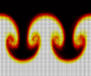
Figure 1. Evolution of the lower-order  $z$-model, starting from a Gaussian perturbation of a flat interface, run on a $192\times 192$ mesh in 18 s.

Figure 2. Evolution of the higher-order  $z$-model, starting from a Gaussian perturbation of a flat interface, run on a $192\times 192$ mesh in 420 s. Note that the lower-order $z$-model (figure 1) traces a sort of ‘envelope’ for the higher-order $z$-model.
The first term of the Laurent series for  $\boldsymbol \omega (s')\times (\boldsymbol z(s)-\boldsymbol z(s'))/|z(s)-z(s')|^3$ is given by (2.40) with an error which is $O(|s-s'|^{-1})$ as $s' \to s$. The $O(|s-s'|^{-1})$ term in this expansion is what remains in (2.39), and upon integration in $s'$, produces a leading-order estimate for the error or remainder $\mathcal {R}$ between the lower-order velocity $\tilde {\boldsymbol u}$ and the full Birkhoff–Rott velocity $\bar {\boldsymbol u}$. Utilizing our isotropy assumption shows that
 \begin{align}
\mathcal{R}&=\frac{\partial_\beta(\sqrt h\boldsymbol
n)R^\beta R^\alpha{\mu}_\alpha}{|h|^{3/2}}
-\frac{1}{2}\frac{h^{\gamma\delta}(\partial_{\alpha\beta}\boldsymbol
z\boldsymbol{\cdot}\partial_\gamma\boldsymbol z)R^\beta
R^\alpha{\mu}_\delta}{|h|^{3/2}}\boldsymbol n \nonumber\\
&\quad -\frac{1}{2}\frac{(\boldsymbol n\boldsymbol{\cdot} \partial_{\alpha\beta}\boldsymbol
z)((\partial_1\boldsymbol z\times\boldsymbol n)R^\alpha R^\beta{\mu}_2-(\partial_2\boldsymbol
z\times\boldsymbol n)R^\alpha R^\beta{\mu}_1)}{|h|^{3/2}}\nonumber\\ &\quad
-\frac{3}{2}\frac{(R^\alpha R^\beta R^\gamma
R^\delta{\mu}_\alpha)(\partial_\beta\boldsymbol
z\boldsymbol{\cdot}\partial_{\gamma\delta}\boldsymbol
z)}{|h|^{5/2}}\boldsymbol n.
\end{align}
\begin{align}
\mathcal{R}&=\frac{\partial_\beta(\sqrt h\boldsymbol
n)R^\beta R^\alpha{\mu}_\alpha}{|h|^{3/2}}
-\frac{1}{2}\frac{h^{\gamma\delta}(\partial_{\alpha\beta}\boldsymbol
z\boldsymbol{\cdot}\partial_\gamma\boldsymbol z)R^\beta
R^\alpha{\mu}_\delta}{|h|^{3/2}}\boldsymbol n \nonumber\\
&\quad -\frac{1}{2}\frac{(\boldsymbol n\boldsymbol{\cdot} \partial_{\alpha\beta}\boldsymbol
z)((\partial_1\boldsymbol z\times\boldsymbol n)R^\alpha R^\beta{\mu}_2-(\partial_2\boldsymbol
z\times\boldsymbol n)R^\alpha R^\beta{\mu}_1)}{|h|^{3/2}}\nonumber\\ &\quad
-\frac{3}{2}\frac{(R^\alpha R^\beta R^\gamma
R^\delta{\mu}_\alpha)(\partial_\beta\boldsymbol
z\boldsymbol{\cdot}\partial_{\gamma\delta}\boldsymbol
z)}{|h|^{5/2}}\boldsymbol n.
\end{align}
Using the fact that the Riesz transforms have unit norm as bounded operators on  $L^2$, Hölder's inequality shows that
 \begin{equation} \left(\iint_{\mathbb{R}^2} \mathcal{R} (s)^2\,{\rm d}s\right)^{{{1}/{2}} }\leq C\left(\iint_{\mathbb{R}^2}|\boldsymbol{\mu}(s)|_h^2\, \textrm{d}s\right)^{{1}/{2}}\sum_{\alpha,\beta=1}^2\sup_{s\in \mathbb{T}^2}\frac{|\partial_{\alpha\beta}\boldsymbol z|}{1+|h|}, \end{equation}
where  $|\boldsymbol{\mu} |_h^2=h_{\alpha \beta }{\mu} ^\alpha {\mu} ^\beta$ is the magnitude of $\boldsymbol{\mu}$ with respect to the metric $h$ on $\varGamma (t)$. In more concise notation,
 \begin{equation} \|\mathcal{R} \|_{L^2}\leq\|\boldsymbol{\mu}\|_{L^2} \left\| \frac{D^2z}{|h|^{{3}/{2}}} \right\|_{L^\infty} . \end{equation}
Since the mean curvature vector on  $\varGamma (t)$ is defined as
 \begin{equation} \kappa(s,t) \boldsymbol n= \frac{h^{ \alpha \beta }}{ \sqrt h} \partial_{ \alpha \beta }\boldsymbol z \boldsymbol{\cdot} (\partial_1 z \times \partial_2\boldsymbol z) , \end{equation}
the bound (2.46) becomes small when the mean curvature is very small, as  $\|\boldsymbol{\mu} \|_{L^2}$ remains bounded under this scenario.
Inserting  $\tilde {\boldsymbol u}$ into the Euler equations (2.30) in place of the Birkhoff–Rott velocity gets rid of the problematic time-derivative term $(\bar {\boldsymbol u}\boldsymbol {\cdot }\partial _\alpha \boldsymbol z)_t$, as $\tilde {\boldsymbol u}$ is normal to $\varGamma (t)$, and so $\tilde {\boldsymbol u} \boldsymbol {\cdot } \partial _\alpha \boldsymbol z=0$. This yields the following system of equations:
 $$\begin{gather} \partial_t\boldsymbol z=\tilde{\boldsymbol u}, \quad 0< t\le T, \end{gather}$$
 $$\begin{gather}\partial_t{\mu}_\alpha=A\partial_\alpha(|\tilde{\boldsymbol u}|^2-\tfrac{1}{4}h^{\beta\gamma}{\mu}_\beta {\mu}_\gamma-2gz^3), \quad 0< t\le T, \end{gather}$$
 $$\begin{gather}\boldsymbol z(s,0) =\mathring{\boldsymbol z}(s), \quad {\mu}_\alpha(s,0) = {\mathring{\mu}}_\alpha(s), \end{gather}$$
where  $\mathring {\boldsymbol z}(s)$ and ${\mathring{\mu}} _\alpha (s)$ denote the initial conditions for the interface parameterization and vorticity, respectively. We refer to (2.48) as the lower-order $z$-model. It is an extremely efficient model, which tracks the interface accurately until about the time of turnover, after which it forms a sort of ‘envelope’ for the roll-up in the near-symmetric regime (see figure 1). This envelope behaviour accurately captures the large-scale behaviour of RTI for interfaces with small curvature and small anisotropy, although our medium- and higher-order $z$-models (which are introduced below) are better suited for capturing the small-scale structure of roll-up. In particular, the lower-order $z$-model suppresses interactions between interface points which are close in space but distant in interface variables, i.e. where $|\boldsymbol z(s)-\boldsymbol z(s')|\ll |s-s'|$. This occurs precisely when the interface folds over or rolls up, which is why the model produces poorer results after interface turnover. At a point of high curvature, where the interface folds over itself, the full Birkhoff–Rott velocity correctly gives a large velocity and causes the interface to roll-up further, whereas the lower-order velocity remains small.
We note that a convenient feature of the lower-order  $z$-model (2.48) is that the velocity $\tilde {\boldsymbol u}$ is given by a Fourier multiplier. As such, the numerical implementation of (2.48) can take advantage of the fast Fourier transform which is both fast and easy to implement, and is one of advantages of this model in comparison with the higher-order models to be introduced next. The computational speed of the lower-order $z$-model creates an efficient and effective tool for determining large-scale features of RTI structures, such as interface growth rates and bubble and spike positions. On average, the lower-order $z$-model runs approximately 15 000 times faster than standard numerical schemes for 3-D hydrodynamics (J. Reisner, private communication 2020).
2.4. The 3-D medium-order and higher-order $z$-models

The isotropy assumption made in the derivation of the lower-order  $z$-model is too restrictive for a large class of initial data. As such, we turn our attention to the medium-order $z$-model (2.49) and higher-order $z$-model (2.50). The medium-order $z$-model is obtained by replacing the localized velocity (2.43) with the regularized Birkhoff–Rott velocity (2.18) only in the $z$-evolution equation in (2.48a) while keeping the vorticity equation (2.48b) unchanged:
 $$\begin{gather} \partial_t\boldsymbol z=\bar{\boldsymbol u}^\epsilon, \quad 0< t\le T , \end{gather}$$
 $$\begin{gather}\partial_t{\mu}_\alpha=A\partial_\alpha(|\tilde{\boldsymbol u}|^2-\tfrac{1}{4}h^{\alpha\beta}{\mu}_\alpha {\mu}_\beta-2gz^3), \quad 0< t\le T , \end{gather}$$
 $$\begin{gather}\boldsymbol z(s,0) =\mathring{\boldsymbol z}(s) , \quad {\mu}_\alpha(s,0) = {\mathring{\mu}}_\alpha(s) . \end{gather}$$
For the higher-order  $z$-model, we replace the localized velocity with the regularized Birkhoff–Rott velocity in both equations of (2.48) to obtain
 $$\begin{gather} \partial_t\boldsymbol z=\bar{\boldsymbol u}^\epsilon \quad 0< t\le T , \end{gather}$$
 $$\begin{gather}\partial_t{\mu}_\alpha=A\partial_\alpha(|\bar{\boldsymbol u}^\epsilon|^2-\tfrac{1}{4}h^{\alpha\beta}{\mu}_\alpha {\mu}_\beta-2gz^3) ,\quad 0< t\le T , \end{gather}$$
 $$\begin{gather}\boldsymbol z(s,0) =\mathring{\boldsymbol z}(s) , \quad {\mu}_\alpha(s,0) = {\mathring{\mu}}_\alpha(s) . \end{gather}$$
The medium- and higher-order  $z$-models are able to capture the fine-scale structures of RTI, including the Kelvin–Helmholtz roll-up regions (see figure 2), but are more costly to simulate numerically than the lower-order $z$-model. Nevertheless, the medium- and higher-order $z$-models run $600$ times faster than standard numerical methods for 3-D gas dynamics codes (J. Reisner, private communication 2020).
The evolution equations for the higher-order  $z$-model differ from the integral form of the Euler equations by only one term. In particular, a comparison of the right-hand sides of (2.32b) with (2.50b) shows that the higher-order $z$-model does not have the problematic nonlinear and non-local time-derivative term $2A\partial _t(\bar {\boldsymbol u}\boldsymbol {\cdot }\partial _\alpha \boldsymbol z)$. As we will explain in § 2.5, the reason that the higher-order $z$-model maintains accuracy is that this time-derivative term tends to be small. We note that for the numerical simulations we consider in this work, results from the medium-order $z$-model and the higher-order $z$-model are essentially indistinguishable (compare the first and second rows in figure 10), but the higher-order $z$-model is more numerically stable. For this reason, we have chosen not to report results from the medium-order $z$-model (with the exception of the second row in figure 10).
An important feature of RTI is the differing behaviour of ‘bubbles’ of light fluid rising into the heavy fluid and ‘spikes’ of heavy fluid falling into the light fluid. Our model accurately captures this differing behaviour with the spikes being thinner and slightly longer than the bubbles. Figure 3 shows the evolution of the initial conditions
 \begin{equation} z^1=s^1,\quad z^2=s^2,\quad z^3=\pm0.05{\rm e}^{ - 9|s|^2},\quad {\mu}_1={\mu}_2=0, \end{equation}
at two, three, and four characteristic times.

Figure 3. Cross-sections of the 3-D higher-order  $z$-model, run on a $64\times 64$ grid, with Atwood number $0.7$ and a runtime of 50 s.
2.5. Dynamics of vorticity
The relationship between the components of vorticity  $\omega ^\alpha$ and the interface roll-up is quite straightforward. Each ‘roll’ of the interface corresponds to a sequence of successively stronger concentric ‘ridges’ in the magnitude of vorticity, and the vector field $(\omega ^1,\omega ^2)$ circulates around these ridges. Figure 4 shows a simulation of the higher-order $z$-model (2.50) in which a single ring of vorticity (top row, pre-turnover) splits into two rings of vorticity, the inner ring stronger than the outer (bottom row, post-turnover). Figure 5 shows the corresponding magnitude of vorticity for the interfaces in figure 4. These spikes in the vorticity are essential to the roll-up of the interface $\varGamma (t)$, but they are also a source of numerical instability. To mitigate this instability, we introduce a smooth, vorticity-scaled, nonlinear artificial viscosity, outlined in § 3.1.

Figure 4. Non-dimensionalized components of vorticity for the higher-order  $z$-model, compared with the full interface. Colour on the interface indicates magnitude of vorticity (red is higher, blue is lower).

Figure 5. Heatmap of the non-dimensionalized magnitude of vorticity for the two interfaces shown in figure 4.
The lower-order  $z$-model fails to roll-up because only one sufficiently strong ring of vorticity can form during the entire evolution. A secondary (weaker) ring of vorticity may form inside the first, but its amplitude is too small to initiate secondary turnover. This weak secondary vorticity produced by the lower-order $z$-model is shown in figure 6.

Figure 6. Non-dimensionalized components of vorticity for the lower-order  $z$-model, compared with the full interface. Colour on the interface indicates magnitude of vorticity (red is higher, blue is lower).
We can now provide a heuristic argument as to why the problematic time-derivative term  $2A\partial _t(\bar {\boldsymbol u}\boldsymbol {\cdot }\partial _\alpha \boldsymbol z)$ on the right-hand side of (2.32b) does not significantly alter the true dynamics, and thus allows for the higher-order $z$-model evolution to accurately simulate solutions of the Euler equations. Integrating (2.32b), we have that
 \begin{align} {\mu}_\alpha(s,
t) & = {\mathring{\mu}}_\alpha(s) + A \int_0^t
\partial_\alpha(|\bar{\boldsymbol u}|^2-\tfrac{1}{4}h^{\beta\gamma}{\mu}_\beta
{\mu}_\gamma-2gz^3) \,\textrm{d}t' \nonumber\\ &
\quad + 2A ( \bar{\boldsymbol u}^\epsilon(s,0)
\boldsymbol{\cdot} \partial_\alpha \mathring z (s) -
\bar{\boldsymbol
u}(s,t)\boldsymbol{\cdot}\partial_\alpha\boldsymbol z(s,t)
) . \end{align}
\begin{align} {\mu}_\alpha(s,
t) & = {\mathring{\mu}}_\alpha(s) + A \int_0^t
\partial_\alpha(|\bar{\boldsymbol u}|^2-\tfrac{1}{4}h^{\beta\gamma}{\mu}_\beta
{\mu}_\gamma-2gz^3) \,\textrm{d}t' \nonumber\\ &
\quad + 2A ( \bar{\boldsymbol u}^\epsilon(s,0)
\boldsymbol{\cdot} \partial_\alpha \mathring z (s) -
\bar{\boldsymbol
u}(s,t)\boldsymbol{\cdot}\partial_\alpha\boldsymbol z(s,t)
) . \end{align}
From (2.40) and the definition of  $\bar {\boldsymbol u}$ given in (2.16), we see that, for $\alpha =1,2$,
 \begin{align} \bar{\boldsymbol u}
\boldsymbol{\cdot} \partial_\alpha\boldsymbol z &=
\iint_{\mathbb{R}^2 }
\frac{(s^\nu-s'^\nu)(s^\beta-s'^\beta)}{|s-s'|^3}\left({\mu}_\nu(s')
\sqrt h\partial_\beta\boldsymbol
n-\frac{1}{2}\left({\mu}_2(s')\partial_1\boldsymbol
z\vphantom{\frac{1}{2}}\right.\right.\nonumber\\
&\left.\left.\quad-{\mu}_1(s')\partial_1\boldsymbol
z\vphantom{\frac{1}{2}}\right)\times\boldsymbol
n(\partial_{\nu\beta}z\boldsymbol{\cdot} n)\vphantom{\frac{1}{2}}\right)
\boldsymbol{\cdot} \partial_\alpha\boldsymbol z
\,\textrm{d}s' \nonumber\\ &= - \iint_{\mathbb{R}^2
}\frac{(s^\nu-s'^\nu)(s^\beta-s'^\beta)}{|s-s'|^3}\left({\mu}_\nu(s')
h^{\delta \nu}\partial_\delta
z\vphantom{\frac{1}{2}}\right.\nonumber\\ &\left.\quad
+\frac{1}{2}({\mu}_2(s')\partial_1\boldsymbol
z-{\mu}_1(s')\partial_1\boldsymbol z)\times n\right)
\boldsymbol{\cdot} \partial_\alpha\boldsymbol z \
(\partial_{\nu\beta}\boldsymbol
z\boldsymbol{\cdot}\boldsymbol n)\,\textrm{d}s',
\end{align}
\begin{align} \bar{\boldsymbol u}
\boldsymbol{\cdot} \partial_\alpha\boldsymbol z &=
\iint_{\mathbb{R}^2 }
\frac{(s^\nu-s'^\nu)(s^\beta-s'^\beta)}{|s-s'|^3}\left({\mu}_\nu(s')
\sqrt h\partial_\beta\boldsymbol
n-\frac{1}{2}\left({\mu}_2(s')\partial_1\boldsymbol
z\vphantom{\frac{1}{2}}\right.\right.\nonumber\\
&\left.\left.\quad-{\mu}_1(s')\partial_1\boldsymbol
z\vphantom{\frac{1}{2}}\right)\times\boldsymbol
n(\partial_{\nu\beta}z\boldsymbol{\cdot} n)\vphantom{\frac{1}{2}}\right)
\boldsymbol{\cdot} \partial_\alpha\boldsymbol z
\,\textrm{d}s' \nonumber\\ &= - \iint_{\mathbb{R}^2
}\frac{(s^\nu-s'^\nu)(s^\beta-s'^\beta)}{|s-s'|^3}\left({\mu}_\nu(s')
h^{\delta \nu}\partial_\delta
z\vphantom{\frac{1}{2}}\right.\nonumber\\ &\left.\quad
+\frac{1}{2}({\mu}_2(s')\partial_1\boldsymbol
z-{\mu}_1(s')\partial_1\boldsymbol z)\times n\right)
\boldsymbol{\cdot} \partial_\alpha\boldsymbol z \
(\partial_{\nu\beta}\boldsymbol
z\boldsymbol{\cdot}\boldsymbol n)\,\textrm{d}s',
\end{align}where we have used the identity
 \begin{equation} \partial_\beta\boldsymbol n = - h^{\delta \nu} ( \partial_{\nu \beta}\boldsymbol{z} \boldsymbol{\cdot}\boldsymbol n) \partial_\delta\boldsymbol z , \end{equation}
and the fact that
 \begin{equation} |s-s'|^3= (h_{\nu\beta}(s)(s^\nu-s'^\nu)(s^\beta-s'^\beta))^{{3}/{2}}. \end{equation}
Since the inner product of the first-order term in (2.40) with  $\partial _\alpha \boldsymbol z$ vanishes,
 \begin{equation} \frac{(s^\nu-{s'}^\nu)}{ |s-s'|^3} {\mu}_\nu(s')\sqrt{h(s)}\boldsymbol n(s)\boldsymbol{\cdot} \partial_\alpha\boldsymbol z =0, \end{equation}
the second-order correction is thus given by
 \begin{align}
\frac{(s^\nu-s'^\nu)}{|s-s'|^3}
(s^\beta-s'^\beta)({\mu}_\nu(s') h^{\delta
\nu}\partial_\delta\boldsymbol z
+\tfrac{1}{2}({\mu}_2(s')\partial_1\boldsymbol
z-{\mu}_1(s')\partial_1\boldsymbol
z)\times\boldsymbol n) \boldsymbol{\cdot}
\partial_\alpha\boldsymbol z \
(\partial_{\nu\beta}\boldsymbol
z\boldsymbol{\cdot}\boldsymbol n) .
\end{align}
\begin{align}
\frac{(s^\nu-s'^\nu)}{|s-s'|^3}
(s^\beta-s'^\beta)({\mu}_\nu(s') h^{\delta
\nu}\partial_\delta\boldsymbol z
+\tfrac{1}{2}({\mu}_2(s')\partial_1\boldsymbol
z-{\mu}_1(s')\partial_1\boldsymbol
z)\times\boldsymbol n) \boldsymbol{\cdot}
\partial_\alpha\boldsymbol z \
(\partial_{\nu\beta}\boldsymbol
z\boldsymbol{\cdot}\boldsymbol n) .
\end{align}
Now, either the curvature of  $\varGamma (t)$ is small in which case $\partial _{\nu \beta }\boldsymbol z\boldsymbol {\cdot }\boldsymbol n$ is small and hence $\bar {\boldsymbol u} \boldsymbol {\cdot } \partial _\alpha \boldsymbol z$ is small, or the curvature is large, in which case the vorticity measure forms highly concentrated peaks (as seen in figure 4), in which the support of the peaks, which is a good approximation for $|s^\beta -s'^\beta |$, is very small. Hence, we see from (2.57) that either small curvature or strongly concentrated vorticity peaks produces small tangential velocity components.
3. Numerical simulation and validation against experiments
In this section we describe the numerical method for solving the  $z$-models, simulate a variety of classical test problems in the RTI, and validate our higher-order $z$-model to against experimental data of single-mode and random multi-mode RTI.
3.1. Numerical approximation of the $z$-model

The boundary integral formulation of the Euler equations, relying on a parametrization of the material interface, has several attractive features for simulating RTI. It is naturally adaptive, concentrating grid points near regions of physical interest, it avoids the numerical diffusion of grid-based methods and it involves fewer independent variables. However, these benefits come at a significant computational cost, due to the nonlinear and non-local form of the time derivatives in this formulation. The use of standard time-stepping algorithms for evolution equations in which the time derivatives are linear and isolated cannot be used. Rather, simulating such equations requires either the solution of a nonlinear Fredholm integral equation of the second kind for the time derivatives, or the use of an iterative predictor–corrector method to evolve forward in time. Additionally, because the non-local expression requires  $O(N^2)$ operation to evaluate (where $N$ is the number of interface points), such predictor–corrector methods extremely expensive. The higher-order $z$-model has nearly all the aforementioned benefits of the full Euler equations in boundary integral form, and can be solved numerically with straightforward finite differencing in space and Runge–Kutta integration in time, with only a small cost in accuracy (see § 2.5).
Geometric complexity is an essential feature of RTI, especially in three space dimensions, so accurately simulating such behaviour requires maintaining a sharp discontinuity in density across the interface, while at the same time faithfully representing the interface geometry at a subgrid scale. The rectangular cells of Eulerian differencing schemes are ill suited to the highly curved geometry of RTI problems, and often introduce spurious KHI spirals which obscure the form of the primary instability. Indeed, a look at the bewildering variety of behaviours observed in the excellent comparative study of Liska & Wendroff (Reference Liska and Wendroff2003) demonstrates that high-order methods such as weighted essentially non-oscillatory methods (WENO) and piecewise parabolic method (PPM), set on structured Cartesian meshes, can be susceptible to spurious small-scale KHI. Nonetheless, for problems which must take into account many physical effects, such as compressibility, thermodynamics, combustion or electromagnetism, methods such as these provide the best available numerical methods. See Zhou et al. (Reference Zhou2021) §§ 5 and 6 for a recent overview of numerical approaches to RTI. Methods such as marker-and-cell (Daly Reference Daly1967) and volume-of-fluid (Hirt & Nichols Reference Hirt and Nichols1981) use either marker particles or a marker function in addition to an Eulerian grid to track the interface. Similarly, front-tracking methods, which use a triangular mesh that advects with the fluid velocity, have shown considerable success (Unverdi & Tryggvason Reference Unverdi and Tryggvason1992; Glimm et al. Reference Glimm, Grove, Li, Shyue, Zeng and Zhang1998).
We now describe our numerical method for the  $z$-models. All computations are set on a uniform spatial grid $\{(i\delta,j\delta ):i,j=-n,\ldots,n-1,n\}$, and the dynamical variables are stored as matrices of values on this grid, e.g.
 \begin{equation} \boldsymbol z_{ij}(t)=\boldsymbol z(i\delta,j\delta,t),\quad i,j= - n,\ldots,n-1,n. \end{equation}
Spatial derivatives are computed using fourth-order centred-difference operators  $(\boldsymbol{\mathsf{D}}_1,\boldsymbol{\mathsf{D}}_2)$. These are used to compute the discretized form of the normal vector $\boldsymbol N=(\boldsymbol{\mathsf{D}}_1\boldsymbol z)\times (\boldsymbol{\mathsf{D}}_2\boldsymbol z)$ and the metric determinant $|h|=|\boldsymbol N|^2$.
For the lower-order  $z$-model, we compute $\tilde {\boldsymbol u}$ via the fast Fourier transform
 \begin{equation} {\tilde{\boldsymbol u}}_{jk}=\mathscr F^{ - 1}\left(\frac{{\textrm{i}}l({\mathscr F}{\mu}_1)_{lm}+{\textrm{i}}m({\mathscr F}{\mu}_2)_{lm}}{(l^2+m^2)^{{1}/{2}}}\right)_{jk}\frac{{\boldsymbol N}_{jk}}{|h|_{jk}^{3/2}} . \end{equation}
This still leaves  $({\mathscr F}{\tilde {\boldsymbol u}})_{00}$ undefined, so we set it to zero. To mitigate the large spikes in vorticity discussed in § 2.5, we introduce a nonlinear artificial viscosity operator $\nu \boldsymbol {\nabla }\boldsymbol {\cdot }(c\boldsymbol {\nabla }/\sup c)$ on the right-hand side of the vorticity equations, where
 \begin{equation} c=(1-\nu\delta^2\Delta)^{ - 1}|\boldsymbol\omega| , \end{equation}
where  $\delta$ is the grid size and $\nu >0$ denotes the artificial viscosity parameter. The function $c$ is a smoothed version of the magnitude of vorticity $|\boldsymbol \omega |$, which provides a smooth localization for the addition of nonlinear artificial viscosity, motivated by the nonlinear (space–time smooth) artificial viscosity method introduced in Reisner, Serencsa & Shkoller (Reference Reisner, Serencsa and Shkoller2013) and utilized in Ramani, Reisner & Shkoller (Reference Ramani, Reisner and Shkoller2019a,Reference Ramani, Reisner and Shkollerb) but employing an elliptic solver at each time step rather than the solution of a parabolic reaction–diffusion equation. This yields the following set of ODEs for the discretized lower-order $z$-model:
 $$\begin{gather} \frac{\textrm{d}\boldsymbol z_{jk}}{\textrm{d}t}=\tilde{\boldsymbol u}_{jk} , \end{gather}$$
 $$\begin{gather}\frac{\textrm{d}\boldsymbol{\mu}_{jk}}{\textrm{d}t}=A\left[\binom{\boldsymbol{\mathsf{D}}_1}{\boldsymbol{\mathsf{D}}_2}\left(|\tilde{\boldsymbol
u}|^2-\tfrac{1}{4}
h^{\alpha\beta}{\mu}_\alpha{\mu}_\beta-2gz^3\right)\right]_{jk}+\nu\left[\sum_{\alpha=1}^2\boldsymbol{\mathsf{D}}_\alpha\left(\frac{c\boldsymbol{\mathsf{D}}_\alpha{\mu}}{\sup
c}\right)\right]_{jk} ,
\end{gather}$$
$$\begin{gather}\frac{\textrm{d}\boldsymbol{\mu}_{jk}}{\textrm{d}t}=A\left[\binom{\boldsymbol{\mathsf{D}}_1}{\boldsymbol{\mathsf{D}}_2}\left(|\tilde{\boldsymbol
u}|^2-\tfrac{1}{4}
h^{\alpha\beta}{\mu}_\alpha{\mu}_\beta-2gz^3\right)\right]_{jk}+\nu\left[\sum_{\alpha=1}^2\boldsymbol{\mathsf{D}}_\alpha\left(\frac{c\boldsymbol{\mathsf{D}}_\alpha{\mu}}{\sup
c}\right)\right]_{jk} ,
\end{gather}$$
which are solved using a total variation decreasing third-order Runge–Kutta method in time. For a generic system of ODEs  $d\boldsymbol x/dt=\boldsymbol f(\boldsymbol x,t)$, the three-step Runge–Kutta method we use to advance the solution from $\boldsymbol x_n=\boldsymbol x(t)$ to $\boldsymbol x_{n+1}=\boldsymbol x(t+\Delta t)$ is given by
 $$\begin{gather} \boldsymbol k_1=\boldsymbol x_n+\Delta t\boldsymbol f(\boldsymbol x_n,t), \end{gather}$$
 $$\begin{gather}\boldsymbol k_2=\frac{3}{4}\boldsymbol x_n+\frac{1}{4}\boldsymbol k_1+\frac{\Delta t}{4}\boldsymbol f(\boldsymbol k_1,t), \end{gather}$$
 $$\begin{gather}\boldsymbol x_{n+1}=\frac{1}{3} \boldsymbol x_n+\frac{2}{3}\boldsymbol k_2+\frac{2\Delta t}{3}\boldsymbol f(\boldsymbol k_2,t+\tfrac{1}{2}\Delta t). \end{gather}$$
 For both the medium- and higher-order  $z$-models, we compute the Birkhoff–Rott velocity $\bar {\boldsymbol u}$ using a Simpson's rule quadrature, which has the form
 \begin{align} \bar{\boldsymbol u}^\epsilon_{ij}=\tfrac{1}{4{\rm \pi}}\sum_k\sum_lM_{kl}\boldsymbol\omega_{kl}\times\frac{\boldsymbol z_{ij}-\boldsymbol z_{kl}}{(\epsilon^2+|\boldsymbol z_{ij}-\boldsymbol z_{kl}|^2)^{3/2}},\quad\boldsymbol\omega_{kl}=({\mu}_{2,kl}(\boldsymbol{\mathsf{D}}_1\boldsymbol z)_{kl}-{\mu}_{1,kl}(\boldsymbol{\mathsf{D}}_2\boldsymbol z)_{kl}) , \end{align}
for some matrix of weights  $\boldsymbol{\mathsf{M}}=(M_{ij})$. The discretized medium-order $z$-model is given by
 $$\begin{gather} \frac{\textrm{d}\boldsymbol z_{jk}}{\textrm{d}t}=\bar{\boldsymbol u}^\epsilon_{jk} , \end{gather}$$
 $$\begin{gather}\frac{\textrm{d}\boldsymbol{\mu}_{jk}}{\textrm{d}t}=A\left[\binom{\boldsymbol{\mathsf{D}}_1}{\boldsymbol{\mathsf{D}}_2}\left(|\tilde{\boldsymbol u}|^2-\frac{1}{4}h^{\alpha\beta}{\mu}_\alpha{\mu}_\beta-2gz^3\right)\right]_{jk}+\nu\left[\sum_{\alpha=1}^2\boldsymbol{\mathsf{D}}_\alpha\left(\frac{c\boldsymbol{\mathsf{D}}_\alpha{\mu}}{\sup c}\right)\right]_{jk} , \end{gather}$$
and the discretized higher-order  $z$-model is
 $$\begin{gather} \frac{\textrm{d}z_{jk}}{\textrm{d}t}=\bar{\boldsymbol u}^\epsilon_{jk} , \end{gather}$$
 $$\begin{gather}\frac{\textrm{d}\boldsymbol{\mu}_{jk}}{\textrm{d}t}=A\left[\binom{\boldsymbol{\mathsf{D}}_1}{\boldsymbol{\mathsf{D}}_2}(|\bar{\boldsymbol u}^\epsilon|^2-\tfrac{1}{4}h^{\alpha\beta}{\mu}_\alpha{\mu}_\beta-2gz^3)\right]_{jk}+\nu\left[\sum_{\alpha=1}^2\boldsymbol{\mathsf{D}}_\alpha\left(\frac{c\boldsymbol{\mathsf{D}}_\alpha{\mu}}{\sup c}\right)\right]_{jk} . \end{gather}$$
 The time required for the computation of the Birkhoff–Rott velocity  $\bar {\boldsymbol u}$ can be drastically shortened with the use of the fast multipole method. Evaluating $\bar {\boldsymbol u}^\epsilon _{jk}$ for all $j$ and $k$ requires $O(N^2)$ operations, where $N=(2n+1)^2$ is the total number of grid points in the simulation. In contrast, the fast multipole method evaluates in $O(N)$ operations, given a fixed relative accuracy goal. As shown in figure 7, we have verified this performance for interface grid resolutions up to size $N=1024\times 1024$ using the open-source package fmm3d (https://github.com/flatironinstitute/FMM3D).

Figure 7. Measured computation times for the Birkhoff–Rott velocity.
3.2. Convergence of the $z$-model

We note that existence of solutions to the incompressible Euler equations with general vortex sheet initial data is not known, and for certain types of vortex sheet data for which weak solutions can be constructed, such solutions are not unique (see, for example, Székelyhidi Reference Székelyhidi2011). As such different regularizations of the Euler equations will lead to sequences of approximate solutions which, such that if these sequences converge, they may not all converge to the same solution. Sequences of approximate Euler solutions, obtained by using a regularized Birkhoff–Rott velocity, have been shown to converge to (possibly non-unique) solutions of the Euler equations in, for example, Beale & Majda (Reference Beale and Majda1982) and Liu & Xin (Reference Liu and Xin1995, Reference Liu and Xin2001). In particular, numerical simulations suggest that the limiting weak solution depends upon the choice of the velocity regularization (see Baker & Pham Reference Baker and Pham2006; Lopes-Filho et al. Reference Lopes-Filho, Lowengrub, Lopes and Zheng2006; Ramani & Shkoller Reference Ramani and Shkoller2020).
On the other hand, as was shown in Ramani & Shkoller (Reference Ramani and Shkoller2020, figures 8–10), the 2-D  $z$-model exhibits convergence of large-scale averaged quantities such as the spiral roll-up centre, the roll-up radius, the location of the bubble and spike tips and the bubble and spike amplitudes. It is likely that such convergence of large-scale features is independent of the numerical approximation employed, and in this section we show that the 3-D higher-order $z$-model converges in this large-scale sense, in the limit as the desingularization and mesh spacing are taken to zero simultaneously.
Figure 8 demonstrates this large-scale convergence for the 3-D higher-order  $z$-model, using the initial data (2.51a–d). As can be seen, there is convergence of the roll-up radius and the location of the spiral centres on a sequence of $n\times n$ meshes with $n=32,64,128,256$, and with regularization parameter $\epsilon$ proportional to the mesh size.

Figure 8. Convergence of roll-up radius and spiral centres for the 3-D higher-order  $z$-model, as the mesh is refined.
3.3. Single-mode initial data
Sinusoidal perturbations of a flat interface were the first to be studied in the context of RTI, and much of the analytical and experimental study of RTI has focused on understanding the evolution of single-mode initial data beyond the linear regime (see, for instance, Emmons, Chang & Watson Reference Emmons, Chang and Watson1960; Cole & Tankin Reference Cole and Tankin1973; Baker et al. Reference Baker, Meiron and Orszag1984; Goncharov Reference Goncharov2002). Of course, in most application scenarios, the interface is perturbed with many different frequencies, but to understand the single-mode problem is the first step towards understanding the more general problem.
For our first test, we use our higher-order  $z$-model to simulate Wilkinson/Jacobs’ isopropyl alcohol/water experiment ( $A=0.15$). We initialize our $z$-model with initial conditions of the form
 \begin{equation} z^1=s^1,\quad z^2=s^2,\quad z^3=a_0\cos({\rm \pi} k s^1/\lambda)\cos({\rm \pi} k s^2/\lambda),\quad {\mu}_1={\mu}_2=0, \end{equation}
where  $-\lambda \leq s^1,s^2\leq \lambda$ and $k$ is a positive integer. We may regard $\lambda$ as a characteristic length for this problem, and the corresponding characteristic time scale is given by $\tau =(\lambda /Ag)^{{1}/{2}}$. This type of initial data was studied experimentally by Wilkinson and Jacobs, who used planar laser-induced fluorescence to visualize a diagonal cross-section of the fluid as it evolved, showing the double roll-up which distinguishes 3-D RTI from 2-D RTI (Wilkinson & Jacobs Reference Wilkinson and Jacobs2007). Results for the case $k=2$ are shown in figure 9.

Figure 9. Single-mode initial data with two wavelengths along each side of the tank, run using the higher-order  $z$-model on a $192\times 192$ grid, with Atwood number 0.15 and a computation time of 380 s.
Starting from a single-mode perturbation of a flat interface, 3-D RTI forms a periodic pattern of bubbles and spikes in such a way that two vortices form on the side of each bubble or spike. In two dimensions, single-mode RTI produces a stationary row of counter-rotating vortices, which manifests as a single row of roll-up regions. However, in 3-D, single-mode RTI produces two grids of counter-rotating vortex rings, which move apart from each other at roughly constant speed. Upon taking a cross-section along the diagonal of the tank, we obtain the double-spiral pattern seen here. See Chapman & Jacobs (Reference Chapman and Jacobs2006) figures 8 and 16 for a helpful illustration of single vs double roll-up regions.
Using the parameters from their experiments and matching the wavelength of the initial data as best we could, we were able to achieve remarkably good agreement between our higher- and medium-order  $z$-models and their experimental data – see figure 10. As shown in figure 11, the lower-order $z$-model matches the experiments quite well at early times. At later times, however, the lower-order $z$-model cannot capture the full extent of the roll-up, as discussed in § 2.5.

Figure 10. (a,b) Higher-order  $z$-model. (c,d) Medium-order $z$-model. Both were run on $160\times 160$ meshes, with Atwood number 0.15 and a runtime of 270 s. Experimental photographs from Wilkinson & Jacobs (Reference Wilkinson and Jacobs2007). Copyright 2007, AIP Publishing. Reproduced with permission.

Figure 11. Lower-order  $z$-model, run on a $130\times 130$ grid, with Atwood number $0.15$ and a runtime of $9$ s. Experimental photographs from Wilkinson & Jacobs (Reference Wilkinson and Jacobs2007). Copyright 2007, AIP Publishing. Reproduced with permission.
The amplitude of 3-D single-mode RTI initially follows the exponential growth rate  $a\sim \cosh (\sqrt {Agk}t)$ predicted by the linear theory, before slowing to approximately constant velocity. The single-mode model of Goncharov (Reference Goncharov2002) predicts asymptotic bubble and spike velocities of
 \begin{equation} U_b=\sqrt{\frac{2Ag}{(1+A)k}},\quad U_s=\sqrt{\frac{2Ag}{(1-A)k}}, \end{equation}
respectively, where  $k$ is the wavenumber of the initial perturbation. However, an asymptotically constant velocity has been called into question by numerical calculations of Ramaprabhu et al. (Reference Ramaprabhu, Dimonte, Young, Calder and Fryxell2006). Nonetheless, the single-mode experiments of Wilkinson & Jacobs (Reference Wilkinson and Jacobs2007) show a period of linear growth in amplitude near Goncharov's predicted value, before accelerating once again. In figure 12 we have plotted the Froude number (non-dimensional bubble velocity) for the bubbles and spikes in our single-mode experiments,
 \begin{equation} {Fr}_b=\frac{\dot a_b}{\sqrt{\rm \pi} U_b},\quad{Fr}_s=\frac{\dot a_s}{\sqrt{\rm \pi} U_s}, \end{equation}
against the normalized bubble and spike amplitudes  $a_b$ and $a_s$. Although our simulations do not run for as long as the Wilkinson and Jacobs experiments, the Froude numbers are in agreement with the experimental results for the simulated range of amplitudes, showing an increase to slightly above the predicted asymptotic value ${Fr}\sim {\rm \pi}^{-{1}/{2}}$ (compare our figure 12 with figures 15–17 in Wilkinson & Jacobs Reference Wilkinson and Jacobs2007).

Figure 12. Plot of bubble and spike Froude numbers against normalized amplitude for our single-mode RTI simulations. Horizontal line shows asymptotic prediction  ${Fr}\sim {\rm \pi}^{-{1}/{2}}$. Compare with figures 15 and 16 in Wilkinson & Jacobs (Reference Wilkinson and Jacobs2007).
3.4. The 3-D rocket rig experiment
The growth rate of the mixing layer between two fluids subjected to random multi-mode perturbations has been the subject of significant interest and study, and it forms a useful benchmark for our  $z$-models. Starting with a small perturbation of amplitude $h_0$ of a flat interface, theory predicts that the amplitude $h(t)$ of the resulting mixing layer has the form
 \begin{equation} \frac{h-h_0}{\lambda}=\alpha\left(\frac{t}{\tau}\right)^2 , \end{equation}
where  $\alpha$ is a universal growth-rate constant. The growth rate of the interface was tested experimentally by Read (Reference Read1984) and Youngs (Reference Youngs1989), and numerically by Youngs (Reference Youngs1984, Reference Youngs1989). Their experimental set-up consists of a $150\times 150\,\textrm {mm}^2$ tank on a vertical sled, accelerated downward using rocket motors, which gives this experimental set-up the nickname ‘rocket rig’. Read's results suggest that $\alpha$ is between $0.06$ and $0.07$, although individual experiments have given values as low as $0.058$ and as high as $0.077$. To test the higher-order $z$-model in this scenario, we simulate Read's experiment using sodium iodide (NaI) solution $(\rho ^+=1.9\,\textrm {g}\,\textrm {cm}^{-3})$ and pentane $(\rho ^-=0.63\,\textrm {g}\,\textrm {cm}^{-3})$, which results in an Atwood number $A\approx 0.5$. More recently, Ristorcelli & Clark (Reference Ristorcelli and Clark2004) and Cook, Cabot & Miller (Reference Cook, Cabot and Miller2004) independently discovered a new governing equation for the mixing layer amplitude:
 \begin{equation} \dot h^2=C_0Agh. \end{equation}
At large times, the solution to this ODE grows like  $h\sim \tfrac {1}{4}C_0t^2$, so that $C_0=4\alpha$. However, it was found by Cabot & Cook (Reference Cabot and Cook2006) that the ratio $\dot h^2/4Agh$ approaches $\alpha$ only at very long times (around $t=6$- $7\tau$, more than double the runtime of the experiments of Read and Youngs). The numerical experiments of Cabot & Cook (Reference Cabot and Cook2006) ran until $t=30\tau$, or more than eleven times the runtime of Read's experiments, and found that $\alpha$ stabilized at a value of approximately $0.025$. Our numerical experiments were run only for the length of Read's experiments, but the time series plot of $\dot h^2/4Agh$ from our experiments matched that of Cabot & Cook for the length of our experiments. In this article we have simulated the rocket rig using parameter values from Read's NaI/pentane experiment. Two main strategies are possible to initialize the rocket rig for numerical simulations, representing two distinct regimes of instability. The first strategy, case A, is to initialize the instability with a random combination of short-wavelength perturbations, and allow larger-scale disturbances to develop from the nonlinear interaction of the short-wavelength perturbations. The second strategy, case B, is for long-wavelength perturbations to be present in the initial condition, causing the mixing layer to grow more rapidly at early times. See Youngs (Reference Youngs2013) for a more detailed discussion and comparison of the different initialization strategies for the rocket rig. In case A, we initialize our model with a random perturbation of a flat interface, of the form
 \begin{equation} z_1=s_1,\quad z_2=s_2,\quad z_3=A_0\text{Re}\sum_{j_1= - n}^n\sum_{j_2= - n}^na_{j_1,j_2}\exp({\textrm{i}(j_1s_1+j_2s_2)}), \end{equation}
where the complex coefficients  $a_{\boldsymbol j}=a_{j_1,j_2}$ are drawn from a standard normal distribution when $|\boldsymbol j|>n/2$ and zero otherwise, and $A_0$ is chosen so that $(\iint |z_3(s,0)|^2\textrm{d}s)^{{1}/{2}}=0.05$. In case B, we instead draw the coefficients $a_{\boldsymbol j}$ from a normal distribution with variance $\sigma ^2(\boldsymbol j)\propto |\boldsymbol j|^{-3}$.
Figure 13 shows results from 100 simulations of the higher-order  $z$-model, using high-frequency initial perturbations (case A, panel a) or the ‘enhanced mixing’ nonuniform variance (case B, panel b). Both the experiment and the simulation were run for 67.4 ms, or $2.7\tau$. The case A runs show excellent agreement with the value $\alpha =0.06$ suggested by Read's experiments. The computation time was 100 s/run, using $100\times 100$ meshes. The lower-order model does reasonably well also, but the rate of interface growth slows after approximately two characteristic times, because the lower-order $z$-model is not able to fully capture interface roll-up. This is shown in figure 14. All models achieve growth rates around the range found in Read's experiments $(0.058\leq \alpha \leq 0.077)$. We note that, although our simulations do not run long enough to see the stabilization of growth rate $\dot h^2/4Agh\sim \alpha$, they qualitatively match the plot of $\dot h^2/4Agh$ shown in Cabot & Cook up to the runtime of our simulation, showing an increase up to a peak of approximately $0.1$ followed by steady decrease (compare figure 15 to Cabot & Cook Reference Cabot and Cook2006, figure 4). To our knowledge, these are the first interface models which can accurately reproduce the growth rate of disordered RT mixing layers.

Figure 13. Comparison of higher-order  $z$-model with theoretical growth rate, case A (a) and case B (b). The markers show the amplitude growth of the interface, averaged over 100 randomly initialized runs, and the grey bands show one and two standard deviations.

Figure 14. Comparison of lower-order  $z$-model with theoretical growth rate, initialized in case B.

Figure 15. Plot of the time-dependent growth rate  $\dot h^2/4Agh$, averaged over 100 rocket rig runs.
3.5. Fluid mixing in the rocket rig experiment
In addition to measuring the growth rate of the mixing layer, the speed of our high-order  $z$-model simulations makes it feasible to compute ensemble averages of density for randomized initial data as shown in figure 16 for the case of an ensemble of 100 runs. When computing ensembles using the invariant (Gibbs) measure associated with the Euler equations, it is known (Albeverio & Cruzeiro Reference Albeverio and Cruzeiro1990) that ensemble averaging of runs with data using (Gaussian) random frequency fluctuations of the interface produce viscous effects (whose size is inversely proportional to the frequency of perturbation). Such viscous effects can be computed from a uniform ensemble (for the purpose of numerical simulations, it is much easier to compute the uniform ensemble than the ensemble averaging using the invariant measure, but the viscous effects are extremely similar) of runs, and our results for such ensembles (see figure 16) is in good agreement with traditional simulations of RTI using the Navier–Stokes equations.

Figure 16. Ensemble-averaged density for the 100 runs of the rocket rig analysed above, showing a cross-section at  $y=0$.
The horizontally averaged density as a function of the vertical coordinate and time, which we will denote  $\bar \rho (z,t)$, is a useful measurement of the large-scale phenomenology of Rayleigh–Taylor turbulence. While it is expensive to compute this function using DNS, Boffetta et al. (Reference Boffetta, De Lillo and Musacchio2010) showed that the solution to a simple parabolic model equation for $\bar \rho$ using the so-called Prandtl closure model closely matches results from DNS. Our objective is to demonstrate that the ensemble-averaged density field computed from 100 $z$-model runs reproduces results obtained from the Prandtl closure model, and thus also reproduces results from DNS. In particular, we shall demonstrate that the $z$-model, even at low resolution, captures the statistical qualities of turbulent mixing quite accurately and reproduces the remarkable self-similarity of the horizontally averaged density.
Averaging the density transport equation  $\partial _t\rho +\partial _x(\rho u)+\partial _y(\rho v)+\partial _z(\rho w)=0$ over the horizontal ( $x$ and $y$) coordinates results in the equation $\partial _t\bar \rho +\partial _z\overline{\rho w}=0$, where $\bar \rho$ is the horizontally averaged density field given by
 \begin{equation} \bar\rho(z,t)={\int\hskip -1,05em -\,}_{\mathbb{R}^2}\rho(x,y,z,t)\,{\rm d}\kern 0.06em x\,{\rm d}y, \end{equation}
and  $\overline{\rho w}$ is the horizontally averaged vertical mass flux. To close the equation for $\bar \rho$, the Prandtl closure model assumes that $\overline{\rho w}=\kappa \partial _z\bar \rho$, where $\kappa$ is known as the ‘eddy diffusivity’. This eddy diffusivity has units of length $^2$/time, so it is natural to take $\kappa \propto h\dot h$, where $h$ is a characteristic length and $\dot h$ is a characteristic velocity for the turbulent flow. In our case, $h\propto Agt^2$ is the characteristic mixing layer height in the rocket rig, so that
 \begin{equation} \kappa\propto(Ag)^2t^3 . \end{equation}
Letting  $\beta ^2$ denote the dimensionless constant of proportionality, the following evolution equation for $\bar \rho$ is obtained (Boffetta et al. Reference Boffetta, De Lillo and Musacchio2010):
 \begin{equation} \partial_t\bar\rho=(\beta Ag)^2t^3\partial_z^2\bar\rho . \end{equation}
This equation has the similarity variable  $\xi =z/(Agt^2)$, which results in a self-similar solution of the form $\bar \rho (z,t)=P(\xi )$ for the density field in the rocket rig experiment given by
 \begin{equation} P(\xi)=\rho^- +\frac{\rho^+ - \rho^-}{2}\left(1+\text{erf}\left(\frac{\xi}{\beta}\right)\right) . \end{equation}
Note that as  $t\to 0^+$, $P(\xi )$ approaches the step-function initial density
 \begin{equation} \bar\rho(z,0)=\begin{cases} \rho^+, & z>0,\\ \rho^-, & z\leq 0. \end{cases} \end{equation}
As noted above, Boffetta et al. (Reference Boffetta, De Lillo and Musacchio2010) have shown that the self-similar solution  $P(\xi )$ to (3.22) is an accurate approximation to the density field $\bar \rho (z,t)$ computed from fully resolved DNS.
In order to determine if the  $z$-model can capture the self-similar solution of the Prandtl closure model, we shall use the ensemble-averaged density field $\rho$ computed from 100 $z$-model simulations, and then calculate the horizontally averaged density field $\bar \rho (z,t)$. We note that the mass associated with the horizontally averaged density field, given by $\int _{-0.5 \lambda }^{0.5\lambda } \bar \rho (z,t) \,\textrm {d}z$, is approximately conserved; in particular, on the full time interval $0 \le t \le 2.5\tau$ of the numerical experiment, we have verified that mass deviates from its initial value by less than $1\,\%$. A series of time snapshots $\bar \rho ({\cdot },t)$ is plotted in figure 17 at various times between $t=1.3\tau$ and $t=2.5\tau$, at intervals $\Delta t=0.2\tau$. To compare against the self-similar solution $P(\xi )$ in (3.23), we have plotted the curves $\bar \rho (z,t)=\bar \rho (Agt^2\xi,t)$ (for various values of $t$) as a function of $\xi$ in figure 18. Here, $\beta$ is chosen to be the ‘best-fit’ value for the data, which we found to be approximately $\beta =0.017$. As can be seen in figure 18, the $z$-model horizontally averaged density profiles $\bar \rho (z,t)$ enjoy the self-similar profile of the solution $P(\xi )$ produced by the Prandtl closure model, and are thereby compare well with fully resolved DNS.

Figure 17. Horizontally averaged density field  $\bar \rho (z,t)$ for the rocket rig experiment, computed from the ensemble-averaged $z$-model density, plotted at times between $t=1.3\tau$ and $t=2.5\tau$, with time intervals $\Delta t=0.2\tau$.

Figure 18. The same density profiles as in figure 17, plotted as a function of the similarity variable  $\xi =z/(Agt^2)$ and compared against the theoretical solution $P(\xi )$.
We next demonstrate that the ensemble averaging of the  $z$-model density field reproduces optimal mixing rates. As explained in Lin et al. (Reference Lin, Thiffeault and Doering2011) and Thiffeault (Reference Thiffeault2012), the mixing of a passive scalar (in our case the density $\rho$), advected by a velocity field $\boldsymbol u$, can be measured quantitatively using the homogeneous Sobolev norms
 \begin{equation} \|\rho\|_{\dot H^s}=\left(\int_{\mathbb{R}^3}|\boldsymbol k|^{2s}|\hat\rho(\boldsymbol k)|^2\,\textrm{d}\boldsymbol k\right)^{{1}/{2}}, \end{equation}
with  $s<0$. Of particular interest are the so-called mixing norms corresponding to the exponents $s=-1$ and $s=-{1}/{2}$. A fluid becomes molecularly mixed when the varying density field $\rho (x,y,z,t)$ converges to its spatial average $\langle \rho \rangle ={\int\hskip -1,05em -\,} _{\mathbb {R}^3}\rho (x,y,z,t)\,\textrm {d}\kern0.06em x\,\textrm {d}y\,\textrm {d}z$. Lin et al. (Reference Lin, Thiffeault and Doering2011) showed that $\rho ({\cdot },t)$ can converge at most exponentially fast to its average in one of these mixing norms, and showed that optimal mixing is achieved if the density is advected by one of a few simple, explicit ‘stirring’ velocity fields $\boldsymbol u(\boldsymbol x,t)$. However, it is unknown whether optimal mixing is achieved for more general velocity fields, such as those satisfying the Euler or Navier–Stokes equations. That is, optimal mixing occurs if
 \begin{equation} \|\rho( {\cdot } , t) - \langle\rho\rangle\|_{\dot H^s}\sim e^{ - rt}, \ s= - 1 \quad \text{or}\quad s= - \tfrac{1}{2} \end{equation}
for some constant  $r>0$ as time $t\to \infty$ (see Thiffeault Reference Thiffeault2012). By computing the $\dot H^{-{1}/{2}}$ and $\dot H^{-1}$ norms of the ensemble-averaged rocket rig density in a small strip around the plane $z=0$, we find that the Sobolev norms decay exponentially (figure 19). In other words, the ensemble average of $z$-model simulations with randomly perturbed initial data is consistent with optimal mixing of the two fluids. While a single $z$-model simulation approximates the motion a fluid interface separating two inviscid fluids, the ensemble average of many simulations successfully models viscous mixing at the length scales of the random fluctuations of the data. A more in-depth study of mixing rates in Rayleigh–Taylor problems, and in particular whether they achieve optimal mixing, is an objective of our future studies.

Figure 19. Mixing norms of the ensemble-averaged density shown in figure 16, plotted on a log scale.
3.6. Fluid mixing in complex stratifications
In multiphase fluid problem, in which the interface exhibits significant roll-up and small-scale structure formation, the interface can ‘squeeze’ a fluid into a very thin configuration, as the distance between portions of the fluid interface becomes smaller and smaller. The resulting small distance between portions of the interface creates (super-exponential) growth of the density gradient and ensures that traditional numerical schemes, based upon a multi-dimensional discretization of the fluid domains, can become prohibitively expensive due to severe small-scale resolution requirements. Such small-scale formation occurs in many situations when significant KHI is allowed to develop, or when the fluid becomes turbulent. Our interface  $z$-model is designed specifically for this small-scale scenario, in which the use of conventional numerics would not be feasible.
Unstable stratified flows with more than two fluid layers provide an interesting example of such small-scale structure formation. We shall consider the problem of two fluid interfaces separating three fluids, and our initial data are chosen as
 \begin{equation} \boldsymbol u_0(x,y,z)=\boldsymbol 0,\quad\rho_0(x,y,z)=\begin{cases} \rho_3, & z>h_2(x,y),\\ \rho_2, & h_1(x,y)\leq z\leq h_2(x,y),\\ \rho_1, & z< h_1(x,y), \end{cases} \end{equation}
where  $\rho _1<\rho _2<\rho _3$ denote the initial densities of the three fluids, and $h_1$ and $h_2$ are given functions which represent the initial position of the two fluid interfaces. Our $z$-model is easily generalized to simulate such problems by introducing two interfaces $\varGamma _i(t)$, parametrized by $\boldsymbol z_i(s,t)$ and carrying vortex sheet densities $\boldsymbol{\mu} _i(s,t)$, $i=1,2$. Following our derivation of the standard $z$-model, we obtain that, for $i=1,2$,
 $$\begin{gather} \partial_t\boldsymbol z_i(s,t)=\bar{\boldsymbol u}_i(s,t):=\frac{1}{4{\rm \pi}}\sum_{j=1}^2\iint_{\mathbb{R}^2}\frac{{\mu}_{j2}(s',t)\partial_1z_j(s',t)-{\mu}_{j1}(s',t)\partial_2z_j(s',t)}{|z_i(s,t)-z_j(s',t)|^3}\,{\rm d}s' , \end{gather}$$
 $$\begin{gather}\partial_t{\mu}_i(s,t)=A\boldsymbol{\nabla}_s(|\bar{\boldsymbol u}_i(s,t)|^2 -\tfrac{1}{4}g_i^{jk}(s,t){\mu}_{ij}(s,t){\mu}_{ik}(s,t)-2gz_i^3(s,t)) . \end{gather}$$
When the two fluid interfaces roll-up inside one another and the separation distance becomes exceedingly small, the density gradient grows exceedingly large, and traditional numerical schemes based on multi-dimensional grids require enormous resolution to accurately capture the small-scale features of the interface and maintain stability. On the other hand, a small interface separation distance does not impair the numerical stability of our interface model, and a two-interface interaction is used to demonstrate stability under small-scale formation. We consider a 2-D unstably stratified three-fluid flow with densities  $\rho _1=1.8$, $\rho _2=3$, $\rho _3=5$, and with the two interfaces given a sinusoidal perturbation of wavelength $\lambda$ and amplitude $0.01\lambda$, separated by a distance $0.05\lambda$. As shown in figure 20, the unstable stratification accelerates the development of RTI, resulting in strong Kelvin–Helmholtz roll-up with the distance between the two interfaces becoming very small.

Figure 20. Simulation of an unstably stratified flow with densities  $\rho _1=1.8$, $\rho _2=3$, $\rho _3=5$, with a sinusoidal initial perturbation of the lower interface. (a) The full domain. (b) Zoomed-in view of the KHI.
We next use our multiple-interface  $z$-model to study the problem of fluid entrainment. Of interest are the experiments of Jacobs & Dalziel (Reference Jacobs and Dalziel2005), who studied fluid mixing in the case where a layer of light fluid (density $\rho ^-$) is initially sandwiched between two layers of heavy fluid (density $\rho ^+$). For short times, this results in standard RTI in the top interface and stability in the bottom interface; at long times, the turbulent flow in the mixing layer becomes strong enough to disturb the lower interface and entrain some of the heavy fluid in the bottom layer. One of the hypotheses tested by Jacobs and Dalziel is that the horizontally averaged species fraction of light fluid, given by
 \begin{equation} f(z,t)=\int_{\mathbb{R}^2}\frac{\rho^+ - \rho(x,y,z,t)}{\rho^+ - \rho^-}\,{\rm d}\kern 0.06em x\,{\rm d}y, \end{equation}
exhibits an asymptotically self-similar distribution at large times, analogous to the self-similarity of the density field shown in figure 18. (Note that the species fraction differs from the density by an affine transformation. We simply choose to model the species fraction in this section to match the experimental results of Jacobs & Dalziel (Reference Jacobs and Dalziel2005).) However, unlike for the standard rocket rig, the simple Prandtl closure model will not suffice, erroneously predicting vertically symmetric growth in the concentration profile. Instead, one finds that
 \begin{equation} \frac{f(z,t)}{f_{max}(t)} = F(\zeta),\quad\zeta=\frac{z-z_c(t)}{w_{{1}/{2}}(t)}, \end{equation}
where  $z_c(t)$ is the centroid of the distribution $f(z,t)$, $w_{{1}/{2}}(t)$ is the width-at-half-height of $f(z,t)$ and $f_{max}(t)=\max f({\cdot },t)$. Moreover, it was shown by dimensional arguments and verified experimentally by Jacobs & Dalziel (Reference Jacobs and Dalziel2005) that
 \begin{equation} f_{max}\sim \frac{1}{t},\quad w_{{1}/{2}}\sim t, \end{equation}
as  $t\to \infty$. We use our multi-interface $z$-model to compute the concentration curves $f(z,t)$. In particular, we compute the ensemble-averaged density field from 25 $z$-model runs, and compute the horizontally averaged species fraction using the formula (3.30). A selection of the resulting species fraction curves $f(z,t)$, as well as their rescaled counterparts, are shown in figure 21. As can be seen in figure 22, solutions of the $z$-model verify the long-time growth prediction for the functions $w_{{1}/{2}}(t)$ and $1/f_{max}(t)$ given by Jacobs and Dalziel. As seen in figure 22, our computation of the functions $w_{{1}/{2}}(t)$ and $1/f_{max}(t)$ indeed demonstrate long-time linear growth. Thus the presence of a layer of heavy fluid below an unstably stratified density field serves to stabilize the resulting RTI, resulting in linear rather than quadratic growth of the mixing layer.

Figure 21. (a) Mean species fraction  $f({\cdot },t)$, plotted at various times. (b) Mean species fraction, plotted in rescaled coordinates to highlight self-similarity of concentration profiles.

Figure 22. Time evolution of the width-at-half-height  $w_{{1}/{2}}(t)$ (a) and the reciprocal of the maximum concentration $1/f_{max}(t)$ (b), showing linear growth after $t/\tau =3$.
4. Conclusions
We have derived and tested our interface  $z$-model for RTI where the material interface is represented by a parametrized surface in three dimensions, and the velocity is reconstructed using a boundary integral method, by assuming potential flow in the fluid bulk. Using our models, we have studied several classical problems in RTI, including single-mode and random multi-mode initial data. We have demonstrated that ensemble averages of inviscid RTI with random multi-mode initial data reproduce the self-similar vertical density distribution predicted by a simple Prandtl closure model, and achieve the theoretically optimal exponential mixing rate for passive scalar fields. Additionally, the derivation of our one-interface model has been generalized to allow for multiple fluid interfaces, thus permitting the study of unstably stratified fluid flow. We have demonstrated self-similarity of the species fraction profile for a heavy–light–heavy initial distribution of densities, and corroborated the similarity exponents measured experimentally by Jacobs & Dalziel (Reference Jacobs and Dalziel2005). These three-phase fluid problems provide a significant numerical challenge for conventional numerical methods, as the distance between the two interfaces becomes extremely small and the gradient of density becomes extremely large, which our model is able to simulate stably. The idea of dimension reduction via the Birkhoff–Rott integral is now classical, but after more than six decades of simulation efforts, few competitive results exist for 3-D dynamics. We have been able to identify the appropriate modifications for the evolution of the amplitude of vorticity which allow our interface model to avoid severe numerical difficulties and retain high accuracy of the location of vorticity spikes that initial interface roll-up. We have demonstrated the efficacy of these models for single-mode initial data and random multi-mode initial data when compared against experimental data, which shows that two-phase potential flow is sufficiently rich to capture the complexity of 3-D RTI. This makes our model a stable and accurate alternative to the challenging simulations of the full two-phase irrotational and incompressible Euler equations. In the future, we hope to extend this model to include topological transitions in the interface, so we can test the efficacy of our model in late-stage RTI and turbulent mixing, and perform a more detailed study of optimal mixing rates in RTI-driven turbulence.
Acknowledgements
We would like to thank J. Reisner at Los Alamos for many fruitful discussions on the subject of this paper. We are indebted to the anonymous referees whose comments have greatly improved the manuscript.
Funding
Research reported in this publication was supported by NSF grant DMS-2007606 and DTRA grant HDTRA11810022. This research was also supported by Office of Defense Nuclear Nonproliferation Research and Development NA-24 and we note that the views of the authors do not necessarily reflect the views of the USG. This work was also supported by the Laboratory Directed Research and Development Program of the Los Alamos National Laboratory, which is under the auspices of the National Nuclear Security Administration of the U.S. Department of Energy under DOE Contracts W-7405-ENG-36 and LA-UR-10-04291. This research was also supported by Office of Defense Nuclear Nonproliferation Research and Development NA-22.
Declaration of interests
The authors report no conflict of interest.


