


1. Introduction
Helicity (Moreau Reference Moreau1961; Moffatt Reference Moffatt1969; Arnold Reference Arnold2014) is an important global quantity describing the topology of a divergence-free vector field. Intuitively, a flow field with a non-zero helicity can have helical stream or vortex lines. Typical vortex tubes with an axial flow and non-zero helicity were reported in wing-tip vortices (Devenport et al. Reference Devenport, Rife, Liapis and Follin1996; Tong, Yang & Wang Reference Tong, Yang and Wang2020), Taylor–Görtler vortices (Wood, Mehta & Koh Reference Wood, Mehta and Koh1992), streamwise vortices in shear flows (Hall & Sherwin Reference Hall and Sherwin2010; Zhao, Yang & Chen Reference Zhao, Yang and Chen2016; Ruan et al. Reference Ruan, Xiong, You and Yang2022), tornadoes (Kurgansky Reference Kurgansky2017), Langmuir circulations (Moffatt & Tsinober Reference Moffatt and Tsinober1992) and helical coherent structures in turbulence (Tsinober & Levich Reference Tsinober and Levich1983; Hussain Reference Hussain1986; Pelz, Shtilman & Tsinober Reference Pelz, Shtilman and Tsinober1986; Xiong & Yang Reference Xiong and Yang2019a).
In particular, helicity is one of only two quadratic invariants in three-dimensional ideal fluid flows (the other one is kinetic energy). It plays an essential role in the generation and energy cascade of turbulent flows (Arnold Reference Arnold1992; Moffatt & Tsinober Reference Moffatt and Tsinober1992; Moffatt Reference Moffatt2021). André & Lesieur (Reference André and Lesieur1977) showed that a finite helicity can be generated from an initial state with vanishing helicity in decaying isotropic turbulence at high Reynolds numbers, illustrating the prevalence of helicity in turbulent flows. Moffatt (Reference Moffatt2014) and Alexakis & Biferale (Reference Alexakis and Biferale2018) pointed out that helicity can impede the forward energy cascade and even promote the inversion of energy transfer.
Unlike kinetic energy, helicity is not sign definite and its sign is changed by altering the chirality of the coordinate frame. Therefore, helicity is a pseudo-scalar and characterizes the parity breaking of a fluid flow. The parity can be quantified by the helical wave decomposition (HWD) (Constantin & Majda Reference Constantin and Majda1988; Waleffe Reference Waleffe1992). Using the HWD, Chen, Chen & Eyink (Reference Chen, Chen and Eyink2003a) and Chen et al. (Reference Chen, Chen, Eyink and Holm2003b) studied the joint cascade of energy and helicity in three-dimensional turbulence, and conjectured the asymptotic restoration of parity symmetry at small scales. Yang, Su & Wu (Reference Yang, Su and Wu2010) and Yang & Wu (Reference Yang and Wu2011) extended the HWD to an arbitrary single-connected domain. Zhu, Yang & Zhu (Reference Zhu, Yang and Zhu2014) studied purely helical absolute equilibria of incompressible turbulence with the HWD. Alexakis (Reference Alexakis2017) investigated the interaction between different helical modes in turbulent flows, based on a decomposition of energy and helicity fluxes. Yan et al. (Reference Yan, Li, Yu, Wang and Chen2020) proposed the dual-channel helicity cascade as a mechanism of hindered or inverse energy cascade. However, the specific role of helicity in three-dimensional turbulence remains an open problem (Chen et al. Reference Chen, Chen and Eyink2003a; Yao & Hussain Reference Yao and Hussain2022).
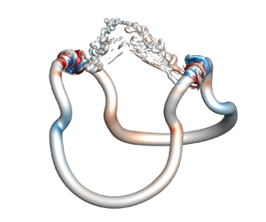
Since helicity can vary in viscous flows, its dynamics has been extensively investigated during topological change, e.g. viscous reconnection (Kida & Takaoka Reference Kida and Takaoka1994; Yao & Hussain Reference Yao and Hussain2022), of a trefoil knotted vortex tube with simple initial geometry and non-trivial topology in numerical simulations (e.g. Kida & Takaoka Reference Kida and Takaoka1987; Ricca, Samuels & Barenghi Reference Ricca, Samuels and Barenghi1999; Scheeler et al. Reference Scheeler, Kleckner, Proment, Kindlmann and Irvine2014; Kerr Reference Kerr2018; Xiong & Yang Reference Xiong and Yang2019a; Yao, Yang & Hussain Reference Yao, Yang and Hussain2021; Zhao et al. Reference Zhao, Yu, Chapelier and Scalo2021; Shen et al. Reference Shen, Yao, Hussain and Yang2022) and experiments (e.g. Kleckner & Irvine Reference Kleckner and Irvine2013; Scheeler et al. Reference Scheeler, Kleckner, Proment, Kindlmann and Irvine2014). Kida & Takaoka (Reference Kida and Takaoka1987, Reference Kida and Takaoka1988) reported that helicity decays in the entire evolution at a low Reynolds number  $\mathit {Re}=1200$, and the decay rate decreases with increasing $\mathit {Re}$, implying that helicity may be conserved in the inviscid limit. By contrast, the recent direct numerical simulation (DNS) of trefoil vortex knots (Yao et al. Reference Yao, Yang and Hussain2021; Zhao & Scalo Reference Zhao and Scalo2021; Zhao et al. Reference Zhao, Yu, Chapelier and Scalo2021) and Hopf links (Yao et al. Reference Yao, Shen, Yang and Hussain2022) at high Reynolds numbers found a ‘transient growth’ of helicity when vortex reconnection occurs, implying that helicity is not conserved in the inviscid limit. Since helicity and its time derivative are not positive definite, the study of helicity in limiting conditions appears to be more challenging than that of kinetic energy or the mean dissipation rate (Batchelor Reference Batchelor1953; Sreenivasan Reference Sreenivasan1984, Reference Sreenivasan1998; Kaneda et al. Reference Kaneda, Ishihara, Itakura and Uno2003). Thus, there is no consensus on whether helicity is conserved in the inviscid limit (Moffatt Reference Moffatt2017; Yao & Hussain Reference Yao and Hussain2022). This open problem inspires us to think from another perspective – how does the flow evolution change if we impose helicity conservation on the Navier–Stokes (NS) equations?
The NS equations were modified to understand some specific roles of helicity. Biferale, Musacchio & Toschi (Reference Biferale, Musacchio and Toschi2012, Reference Biferale, Musacchio and Toschi2013) performed a surgery of the NS dynamics by only keeping the velocity components carrying a well-defined positive or negative helicity, and then they found a stationary inverse energy cascade in homogeneous isotropic turbulence (HIT). Biferale & Titi (Reference Biferale and Titi2013) then demonstrated the global regularity of such helical-decimated NS equations. Furthermore, a series of studies explored the relation between helicity and the direction of energy cascade (e.g. Sahoo, Alexakis & Biferale Reference Sahoo, Alexakis and Biferale2017; Slomka & Dunkel Reference Slomka and Dunkel2017; Alexakis & Biferale Reference Alexakis and Biferale2018; Plunian et al. Reference Plunian, Teimurazov, Stepanov and Verma2020; Alexakis & Biferale Reference Alexakis and Biferale2022). Hao, Xiong & Yang (Reference Hao, Xiong and Yang2019) applied vorticity-based orthogonal decomposition to the non-ideal force in the NS equations, and showed that vortex surfaces can be tracked by a virtual velocity in the modified fluid flow with helicity conservation. She & Jackson (Reference She and Jackson1993) and Gallavotti (Reference Gallavotti1996, Reference Gallavotti1997) discussed another approach to modify the NS equations by introducing integral constraints with a Lagrange multiplier. In this way, the constrained Euler equation (She & Jackson Reference She and Jackson1993) and the Gaussian dissipative Euler equation (Gallavotti Reference Gallavotti1997) with conserved kinetic energy, and the Gaussian NS equation (Gallavotti Reference Gallavotti1996, Reference Gallavotti1997; Jaccod & Chibbaro Reference Jaccod and Chibbaro2021) with conserved enstrophy were obtained. In addition, Bos (Reference Bos2021) kept the enstrophy conserved in turbulence by removing vortex stretching from the NS equations.
In the present study, we investigate the influence of helicity on vortex dynamics and flow statistics by imposing helicity conservation on the NS equations while retaining major NS dynamics. The modified NS equation is referred to as the helicity-conserved Navier–Stokes (HCNS) equation. We then compare the evolutions governed by NS and HCNS equations in various flows to reveal the critical role of helicity. Moreover, the HWD is used to explore the relation between small-scale parity breaking and large-scale helical structures. These efforts can explain the transient helicity variation during vortex reconnection and facilitate flow control by manipulating small-scale flow structures.
The outline of the present paper is as follows. Section 2 introduces the HCNS equation and derives the properties of the HCNS flow. Section 3 studies the HWD of NS and HCNS dynamics. Section 4 describes numerical set-ups and methods. Section 5 compares evolutions of vortical structures and flow statistics in HCNS and NS flows. Some conclusions are drawn in § 6.
2. Theoretical framework of the HCNS flow
2.1. Introduction of the HCNS equation
In a three-dimensional incompressible flow, the velocity  $\boldsymbol {u}(\boldsymbol {x},t)$ is governed by the NS equations
 \begin{gather} \boldsymbol{\nabla}\boldsymbol{\cdot}\boldsymbol{u} = 0, \end{gather}
 \begin{gather}\frac{\partial\boldsymbol{u}}{\partial t} + \boldsymbol{\omega}\times\boldsymbol{u} ={-}\boldsymbol{\nabla}P + \boldsymbol{F}, \end{gather}
where  $\boldsymbol {\omega }\equiv \boldsymbol {\nabla }\times \boldsymbol {u}$ is the vorticity, $P = p/\rho + |\boldsymbol {u}|^2/2 + V_F$ denotes a generalized potential with the pressure $p$, density $\rho$ and potential $V_F$ of conservative body forces and
 \begin{equation} \boldsymbol{F} = \frac{1}{\rho}\boldsymbol{\nabla}\boldsymbol{\cdot}\boldsymbol{\tau} + \boldsymbol{f} \end{equation}
denotes a generalized non-ideal force with viscous stress  $\boldsymbol {\tau }$ and non-conservative external body force $\boldsymbol {f}$ per unit mass. Note that it is straightforward to extend the present analysis to compressible flows (Hao et al. Reference Hao, Xiong and Yang2019).
From (2.2), we obtain the vorticity equation
 \begin{equation} \frac{\partial\boldsymbol{\omega}}{\partial t} + \boldsymbol{\nabla}\times(\boldsymbol{\omega}\times\boldsymbol{u}) = \boldsymbol{\nabla}\times\boldsymbol{F}, \end{equation}
and then the transport equation
 \begin{equation} \frac{\partial h}{\partial t} + \boldsymbol{\nabla}\boldsymbol{\cdot}[P\boldsymbol{\omega} + \boldsymbol{u}\times(\boldsymbol{u}\times\boldsymbol{\omega}) + \boldsymbol{u}\times\boldsymbol{F} ] = 2\boldsymbol{\omega}\boldsymbol{\cdot}\boldsymbol{F} \end{equation}
of the helicity density  $h\equiv \boldsymbol {u}\boldsymbol {\cdot }\boldsymbol {\omega }$.
We impose helicity conservation on the NS equations by modifying the non-ideal force in (2.2), where the helicity (Moreau Reference Moreau1961; Moffatt Reference Moffatt1969)
 \begin{equation} \mathcal{H}(t) \equiv \int_{\mathcal{D}}h\, \mathrm{d} V \end{equation}
is defined over an unbounded domain  $\mathcal {D}$ or that bounded by a vortex surface. To remove the source term of helicity generation, i.e. the right-hand side of (2.5), we apply the vorticity-based orthogonal decomposition (Hao et al. Reference Hao, Xiong and Yang2019) to
 \begin{equation} \boldsymbol{F} = \boldsymbol{F}_\perp + \boldsymbol{F}_\parallel = (\boldsymbol{n}_\omega\times\boldsymbol{F})\times \boldsymbol{n}_\omega + (\boldsymbol{n}_\omega\boldsymbol{\cdot}\boldsymbol{F})\boldsymbol{n}_\omega, \end{equation}
and only keep the orthogonal component  $\boldsymbol {F}_\perp = (\boldsymbol {n}_\omega \times \boldsymbol {F})\times \boldsymbol {n}_\omega$ with $\boldsymbol {n}_\omega \equiv \boldsymbol {\omega }/|\boldsymbol {\omega }|$ in $\boldsymbol {F}$ in (2.2). To avoid the issue of singularity, we define $\boldsymbol {n}_\omega =\boldsymbol {0}$ and $\boldsymbol {F}_\perp =\boldsymbol {F}$ at the points with $|\boldsymbol {\omega }|=0$.
Thus, we obtain the HCNS equation
 \begin{equation} \frac{\partial \boldsymbol{u}}{\partial t} + \boldsymbol{\omega}\times\boldsymbol{u} ={-}\boldsymbol{\nabla}P + (\boldsymbol{n}_\omega\times\boldsymbol{F})\times\boldsymbol{n}_\omega, \end{equation}
and the corresponding vorticity equation
 \begin{equation} \frac{\partial \boldsymbol{\omega}}{\partial t} + \boldsymbol{\nabla}\times(\boldsymbol{\omega}\times\boldsymbol{u}) = \boldsymbol{\nabla}\times[(\boldsymbol{n}_\omega\times\boldsymbol{F})\times\boldsymbol{n}_\omega], \end{equation}
for the HCNS flow governed by (2.8) and (2.1). Note that the HCNS equation degenerates to the NS equation in one and two dimensions, and it has all the symmetry groups (Frisch Reference Frisch1995) of the NS equation.
2.2. Evolution of integral quantities for the HCNS flow
Without loss of generality, we consider viscous, barotropic and incompressible fluid flows without body forces, i.e.  $P = p/\rho + |\boldsymbol {u}|^2/2$ and $\boldsymbol {F} = \nu \nabla ^2\boldsymbol {u}$ with kinematic viscosity $\nu$ below. The corresponding momentum and vorticity equations for the HCNS flow are
 \begin{equation} \frac{\partial\boldsymbol{u}}{\partial t} + \boldsymbol{\omega}\times\boldsymbol{u} ={-}\boldsymbol{\nabla}P + \nu(\boldsymbol{n}_\omega\times\nabla^2\boldsymbol{u})\times\boldsymbol{n}_\omega \end{equation}
and
 \begin{equation} \frac{\partial\boldsymbol{\omega}}{\partial t} + \boldsymbol{\nabla}\times(\boldsymbol{\omega}\times\boldsymbol{u}) = \nu\boldsymbol{\nabla}\times[(\boldsymbol{n}_\omega\times\nabla^2\boldsymbol{u})\times\boldsymbol{n}_\omega], \end{equation}
respectively. Next, we derive transport equations of the total kinetic energy
 \begin{equation} E(t) \equiv \int_{\mathcal{D}}\frac{|\boldsymbol{u}|^2}{2}\, \mathrm{d} V, \end{equation}
enstrophy
 \begin{equation} \varOmega(t) \equiv \int_{\mathcal{D}}\frac{|\boldsymbol{\omega}|^2}{2}\, \mathrm{d} V \end{equation}
and helicity (2.6) for the HCNS flow.
First, the transport equation of the local kinetic energy reads
 \begin{equation} \frac{\mathrm{D}}{\mathrm{D} t}\frac{|\boldsymbol{u}|^2}{2} = \boldsymbol{\nabla}\boldsymbol{\cdot}\left( -\frac{p}{\rho}\boldsymbol{u} + \nu\boldsymbol{u}\times\boldsymbol{\omega} \right) - \nu|\boldsymbol{\omega}|^2 + \nu h\xi_\omega. \end{equation}
Here,  $\mathrm {D}/\mathrm {D} t \equiv \partial /\partial t + \boldsymbol {u}\boldsymbol {\cdot }\boldsymbol {\nabla }$ is the material derivative and $\xi _\omega \equiv \boldsymbol {n}_\omega \boldsymbol {\cdot }(\boldsymbol {\nabla }\times \boldsymbol {n}_\omega )$ denotes the torsion of neighbouring vortex lines (Truesdell Reference Truesdell2018). Integrating (2.14) over $\mathcal {D}$ yields
 \begin{equation} \frac{\mathrm{d} E}{\mathrm{d} t} ={-}2\nu\varOmega + \nu\int_{\mathcal{D}}\xi_u\xi_\omega |\boldsymbol{u}|^2\, \mathrm{d} V, \end{equation}
where  $\xi _u\equiv \boldsymbol {n}_u\boldsymbol {\cdot }(\boldsymbol {\nabla }\times \boldsymbol {n}_u)$, similar to $\xi _\omega$, denotes the torsion of neighbouring streamlines with $\boldsymbol {n}_u\equiv \boldsymbol {u}/|\boldsymbol {u}|$. Note that our discussion is restricted to an unbounded domain or a periodic domain $\mathcal {D}$, otherwise there will be a boundary integral term in (2.15).
We demonstrate that the HCNS flow is dissipative, i.e.  $\mathrm {d} E/\mathrm {d} t\le 0$. Considering $\xi _u(\boldsymbol {x})\xi _\omega (\boldsymbol {x})$ is a continuous function and $|\boldsymbol {u}(\boldsymbol {x})|^2\ge 0$ within $\mathcal {D}$, applying the mean value theorem for integrals to (2.15) yields
 \begin{equation} \frac{\mathrm{d} E}{\mathrm{d} t} ={-}2\nu\varOmega + 2\nu\xi_u^*\xi_\omega^*E, \end{equation}
with  $\xi _{u}^*=\xi _{u}({\boldsymbol {x}}^*)$ and $\xi _{\omega }^*=\xi _{\omega }({\boldsymbol {x}}^*)$ at a particular $\boldsymbol {x}^*$ in $\mathcal {D}$.
For a periodic cube  $\mathcal {D}$, comparing Fourier expansions of $E$ and $\varOmega$ yields
 \begin{equation} \varOmega = \frac{L^3}{2}\sum_{\boldsymbol{k}}k^2|\hat{\boldsymbol{u}}|^2 \ge q_0^2\frac{L^3}{2}\sum_{\boldsymbol{k}}|\hat{\boldsymbol{u}}|^2 = q_0^2E, \end{equation}
where  $L$ denotes the side length of $\mathcal {D}$, $\boldsymbol {k}$ the wavenumber vector, $k\equiv |\boldsymbol {k}|$ the wavenumber magnitude and $\hat {\boldsymbol {u}}=\hat {\boldsymbol {u}}(\boldsymbol {k},t)$ the velocity component in Fourier space. In general, we have $q_0\gg 1$ due to the weight $k^2$ in (2.17), unless the energy spectrum is only non-vanishing at several lowest wavenumbers in a simple flow, e.g. the Taylor–Green initial field (Taylor & Green Reference Taylor and Green1937) with the energy spectrum as a Delta-function. Substituting (2.17) with $q_0\gg 1$, $|\xi _u^*|={O}(1)$ and $|\xi _\omega ^*|={O}(1)$ into (2.16) yields that the HCNS flow is dissipative as
 \begin{equation} \frac{\mathrm{d} E}{\mathrm{d} t} \le -2\nu\varOmega + 2\nu|\xi_u^*||\xi_\omega^*|E \le 2\nu\varOmega\left(\frac{|\xi_u^*||\xi_\omega^*|}{q_0^2} - 1 \right) \le 0. \end{equation}
 Second, we consider the transport of enstrophy. Taking inner product of (2.11) with  $\boldsymbol {\omega }$ yields
 \begin{equation} \frac{\mathrm{D}}{\mathrm{D} t}\frac{|\boldsymbol{\omega}|^2}{2} = \boldsymbol{\omega}\boldsymbol{\cdot}{\boldsymbol{\mathsf{S}}}\boldsymbol{\cdot}\boldsymbol{\omega} + \nu\left\{-\sin^2\vartheta_\omega|\nabla^2\boldsymbol{u}|^2 + \boldsymbol{\nabla}\boldsymbol{\cdot}[\boldsymbol{\omega}\times(\boldsymbol{\nabla}\times\boldsymbol{\omega})] \right\}, \end{equation}
where  ${\boldsymbol{\mathsf{S}}}\equiv (\boldsymbol {\nabla u}+\boldsymbol {\nabla u}^{T})/2$ is the rate-of-strain tensor and
 \begin{equation} \vartheta_\omega \equiv \arccos\frac{\boldsymbol{\omega}\boldsymbol{\cdot}\nabla^2\boldsymbol{u}}{|\boldsymbol{\omega}| |\nabla^2\boldsymbol{u}|} \end{equation}
denotes the angle between  $\boldsymbol {\omega }$ and $\nabla ^2\boldsymbol {u}$. Compared with the NS flow, the prefactor $0\le \sin ^2\vartheta _\omega \le 1$ of the second term on the right-hand side of (2.19) weakens the enstrophy dissipation in the HCNS flow (Hao et al. Reference Hao, Xiong and Yang2019).
By integrating (2.19) over  $\mathcal {D}$, we obtain
 \begin{equation} \frac{\mathrm{d}\varOmega}{\mathrm{d}t} = \mathcal{P}_\varOmega - \mathcal{E}_\varOmega^{\text{HCNS}}, \end{equation}
after some algebra, with the production term
 \begin{equation} \mathcal{P}_\varOmega = \int_\mathcal{D}\nabla^2\boldsymbol{u}\boldsymbol{\cdot}(\boldsymbol{\omega}\times\boldsymbol{u})\, \mathrm{d} V \end{equation}
and the dissipation term
 \begin{equation} \mathcal{E}_\varOmega^{\text{HCNS}} = \nu\int_\mathcal{D} \sin^2\vartheta_\omega|\nabla^2\boldsymbol{u}|^2\, \mathrm{d} V. \end{equation}
Comparing  $\mathcal {E}_\varOmega ^{\text {HCNS}}$ in the HCNS flow and
 \begin{equation} \mathcal{E}_\varOmega^{\text{NS}} = \nu\int_{\mathcal{D}}|\nabla^2\boldsymbol{u}|^2\, \mathrm{d} V \end{equation}
in the NS flow, we have  $\mathcal {E}_{\varOmega }^{\text {HCNS}} \le \mathcal {E}_\varOmega ^{\text {NS}}$ with identical production terms in the two flows. Hence, the integration of (2.21) with time from the same initial condition suggests that
 \begin{equation} \varOmega^{\text{HCNS}}(t) \ge \varOmega^{\text{NS}}(t), \end{equation}
where the superscripts ‘NS’ and ‘HCNS’ denote the quantities in NS and HCNS flows, respectively.
Finally, the general equation (2.5) for the helicity density becomes
 \begin{equation} \frac{\mathrm{D} h}{\mathrm{D} t}= \boldsymbol{\nabla}\boldsymbol{\cdot} [P'\boldsymbol{\omega} - \nu\boldsymbol{u}\times\nabla^2\boldsymbol{u} + \nu(\boldsymbol{n}_\omega\boldsymbol{\cdot}\nabla^2\boldsymbol{u})\boldsymbol{u}\times\boldsymbol{n}_\omega ] \end{equation}
in the HCNS flow, where  $P'\equiv -p/\rho + |\boldsymbol {u}|^2/2$ denotes a modified pressure. Applying the divergence theorem to (2.26) yields
 \begin{equation} \frac{\mathrm{d} \mathcal{H}}{\mathrm{d} t} = \mathop{{\int\!\!\!\!\!\int}\mkern-21mu \bigcirc}\nolimits_{\partial \mathcal{D}}\boldsymbol{n}\boldsymbol{\cdot}[P'\boldsymbol{\omega} - \nu\boldsymbol{u}\times\nabla^2\boldsymbol{u} + \nu(\boldsymbol{n}_\omega\boldsymbol{\cdot}\nabla^2\boldsymbol{u})\boldsymbol{u}\times\boldsymbol{n}_\omega ]\, \mathrm{d} S. \end{equation}
Considering  $\mathcal {D}$ with the vanishing boundary integral, (2.27) is simplified to
 \begin{equation} \frac{\mathrm{d} \mathcal{H}}{\mathrm{d} t} = 0. \end{equation}
Therefore, the HCNS flow has a strong constraint of helicity conservation:
 \begin{equation} \mathcal{H}(t) = \mathcal{H}_0, \quad \forall t\ge 0, \end{equation}
where the subscript ‘0’ denotes a quantity at the initial time.
2.3. Beltramization of the HCNS flow
For a decaying HCNS flow, we show its Beltramization at long times with lower bounds of  $E$ and $\varOmega$, where a Beltrami flow has
 \begin{equation} \boldsymbol{\omega}=\lambda\boldsymbol{u}, \end{equation}
with a constant  $\lambda$. Consider the Schwartz inequality
 \begin{equation} \mathcal{H}^2 \le 4E\varOmega, \end{equation}
for a velocity field with  $\mathcal {H}_0\ne 0$, which takes equal only for (2.30). From (2.29) and (2.31), we have
 \begin{equation} 4E(t)\varOmega(t) \ge \mathcal{H}_0^2 > 0, \end{equation}
which implies that both  $E(t)$ and $\varOmega (t)$ have non-vanishing lower bounds, otherwise one of them must diverge. Substituting (2.17) into (2.32) yields
 \begin{equation} \varOmega \ge \frac12 q_0|\mathcal{H}_0|. \end{equation}
Note that the HCNS flow allows both  $E$ and $\varOmega$ to decay to zero for $\mathcal {H}_0 = 0$, e.g. for highly symmetric flows.
Next, we explore the Beltramization of HCNS flows at  $t\rightarrow \infty$. First, the Beltrami field with (2.30) is a steady-state solution to the HCNS equation. For such a solution, (2.10) with $\boldsymbol {u}$, $\boldsymbol {\omega }$ and $\nabla ^2\boldsymbol {u}$ parallel to each other is simplified to $\partial \boldsymbol {u}/\partial t = \boldsymbol {0}$ with $\mathrm {d}E/\mathrm {d}t=0$. Then, we demonstrate the Beltrami field with (2.30) represents the state of the lowest $E$ in the HCNS flow using the variational principle (Woltjer Reference Woltjer1958).
We seek the minimum  $E$ subject to the helicity conservation in (2.29). By varying a generic function
 \begin{equation} I_E \equiv \int_{\mathcal{D}} [\boldsymbol{u}\boldsymbol{\cdot}\boldsymbol{u} - \lambda_E\boldsymbol{u}\boldsymbol{\cdot}(\boldsymbol{\nabla}\times\boldsymbol{u})]\, \mathrm{d} V, \end{equation}
for  $E$, and applying the divergence theorem yield
 \begin{equation} \delta I_E = 2\int_{\mathcal{D}}(\boldsymbol{u}-\lambda_E\boldsymbol{\nabla} \times\boldsymbol{u})\boldsymbol{\cdot}\delta\boldsymbol{u}\, \mathrm{d} V + \mathop{{\int\!\!\!\!\!\int}\mkern-21mu \bigcirc}\nolimits_{\partial \mathcal{D}}\lambda_E \boldsymbol{n}\boldsymbol{\cdot}(\boldsymbol{u}\times\delta\boldsymbol{u})\, \mathrm{d} S = 0, \end{equation}
with a Lagrangian multiplier  $\lambda _E$. Since $\delta \boldsymbol {u}$ vanishes at $\partial \mathcal {D}$ for a closed domain $\mathcal {D}$, and the surface integral in (2.35) also vanishes for an unclosed domain such as the unbounded domain or periodic box, we obtain
 \begin{equation} \int_{\mathcal{D}}(\boldsymbol{u}-\lambda_E\boldsymbol{\nabla}\times \boldsymbol{u})\boldsymbol{\cdot}\delta\boldsymbol{u}\,\mathrm{d} V = 0. \end{equation}
The vanishing integral (2.36) with an arbitrary  $\delta \boldsymbol {u}$ suggests
 \begin{equation} \boldsymbol{u} = \lambda_E\boldsymbol{\nabla}\times\boldsymbol{u}, \end{equation}
for the minimum  $E$. Therefore, the Beltrami field with (2.30) and $\lambda =\lambda _E^{-1}$ corresponds to the lowest energy state of the HCNS flow. For the dissipative HCNS flow with (2.18) and a non-vanishing lower bound of $\varOmega$ in (2.33), the Beltrami flow is the only possible state at long times. At this state, the Schwartz inequality (2.31) becomes
 \begin{equation} 4E_\infty \varOmega_\infty = \mathcal{H}_0^2, \end{equation}
with  $E_\infty = |\mathcal {H}_0|/(2|\lambda |)$ and $\varOmega _\infty = |\lambda \mathcal {H}_0|/2$. The Beltramization of the HCNS flow can be characterized by the criterion
 \begin{equation} \varLambda_B(t) \equiv \frac{\mathcal{H}^2(t)}{4E(t)\varOmega(t)}\in[0,1]. \end{equation}
The Beltrami flow with (2.38) has  $\varLambda _B = 1$.
3. The HWD of NS/HCNS dynamics
3.1. The HWD
Helicity is the signature of parity breaking in incompressible flows (Chen et al. Reference Chen, Chen and Eyink2003a), and the parity can be characterized by the HWD (Constantin & Majda Reference Constantin and Majda1988; Waleffe Reference Waleffe1992). A divergence-free velocity field has  $\boldsymbol {k} \boldsymbol {\cdot } \hat {\boldsymbol {u}}(\boldsymbol {k})=0$, so $\hat {\boldsymbol {u}}(\boldsymbol {k})$ has two degrees of freedom. In the HWD, two independent degrees of freedom are obtained by projecting the velocity
 \begin{equation} \boldsymbol{u}(\boldsymbol{x}) = \sum_{\boldsymbol{k}}\hat{\boldsymbol{u}}(\boldsymbol{k})\,\mathrm{e}^{\mathrm{i}\boldsymbol{k}\boldsymbol{\cdot}\boldsymbol{x}} = \sum_{\boldsymbol{k}}(u^+\boldsymbol{h}^+ + u^-\boldsymbol{h}^-)\,\mathrm{e}^{\mathrm{i}\boldsymbol{k}\boldsymbol{\cdot}\boldsymbol{x}} \end{equation}
onto two orthogonal helical waves with a definite sign of helicity. Here,  $\boldsymbol {k}=(k_1,k_2,k_3)$ is for a periodic cube of side $L=2{\rm \pi}$, with $k_i=0,\pm 1,\pm 2,\ldots, i=1,2,3$. The helical modes $u^{\pm }(\boldsymbol {k})$ are complex scalars, and
 \begin{equation} \boldsymbol{h}^\pm(\boldsymbol{k}) =\frac{1}{\sqrt{2}}\frac{(\boldsymbol{z}_k \times\boldsymbol{k})\times\boldsymbol{k}}{k|\boldsymbol{z}_k\times\boldsymbol{k}|} \pm \frac{\mathrm{i}}{\sqrt{2}}\frac{\boldsymbol{z}_k\times\boldsymbol{k}}{|\boldsymbol{z}_k \times\boldsymbol{k}|} \end{equation}
are two eigenvectors of the curl operator as  $\mathrm {i}\boldsymbol {k}\times \boldsymbol {h}^\pm (\boldsymbol {k})=\pm k\boldsymbol {h}^{\pm }(\boldsymbol {k})$, where $\boldsymbol {z}_k$ is randomly generated for each $\boldsymbol {k}$, keeping $|\boldsymbol {z}_k\times \boldsymbol {k}|\ne 0$. Note that $\boldsymbol {h}^+$ and $\boldsymbol {h}^-$ have properties $\boldsymbol {h}^\pm (\boldsymbol {k})=\boldsymbol {h}^{\mp *}(\boldsymbol {k})$, $|\boldsymbol {h}^\pm |^2=\boldsymbol {h}^+\boldsymbol {\cdot }\boldsymbol {h}^-=1$ and $\boldsymbol {h}^+\boldsymbol {\cdot } \boldsymbol {h}^+=\boldsymbol {h}^-\boldsymbol {\cdot }\boldsymbol {h}^-=0$, where the superscript ‘*’ denotes the complex conjugate.
Projecting  $\hat {\boldsymbol {u}}$ onto $\boldsymbol {h}^\mp$ yields
 \begin{equation} u^\pm(\boldsymbol{k}) = \hat{\boldsymbol{u}}(\boldsymbol{k})\boldsymbol{\cdot}\boldsymbol{h}^\mp(\boldsymbol{k}) = \frac{1}{L^3}\int_{L^3}\boldsymbol{h}^{{\mp}}(\boldsymbol{k})\boldsymbol{\cdot} \boldsymbol{u}(\boldsymbol{x})\, \mathrm{e}^{-\mathrm{i}\boldsymbol{k}\boldsymbol{\cdot}\boldsymbol{x}}\, \mathrm{d}\kern0.06em \boldsymbol{x}, \end{equation}
where  $u^+$ and $u^-$ are right- and left-handed components, respectively. The vorticity can also be expressed in terms of helical modes as
 \begin{equation} \hat{\boldsymbol{\omega}}(\boldsymbol{k}) = k(u^+(\boldsymbol{k})\boldsymbol{h}^+(\boldsymbol{k}) - u^-(\boldsymbol{k})\boldsymbol{h}^-(\boldsymbol{k})). \end{equation}
The integral quantities have HWDs
 \begin{equation} E(t) = E^+(t)+E^-(t), \quad \varOmega(t) = \varOmega^+(t)+\varOmega^-(t), \quad \mathcal{H}(t) = \mathcal{H}^+(t) - \mathcal{H}^-(t), \end{equation}
with
 \begin{equation} E^{{\pm}} \equiv \frac{L^3}{2}\sum_{\boldsymbol{k}}|u^\pm|^2, \quad \varOmega^{{\pm}} \equiv \frac{L^3}{2}\sum_{\boldsymbol{k}}k^2|u^\pm|^2, \quad \mathcal{H}^{{\pm}} \equiv L^3\sum_{\boldsymbol{k}}k|u^\pm|^2. \end{equation}
3.2. Transient variation of helicity in the NS dynamics
Applying the HWD with (3.1) and (3.3) to the NS equation (2.2) with  $\boldsymbol {F}=\nu \nabla ^2\boldsymbol {u}$ yields the equation for helical modes of velocity as (Waleffe Reference Waleffe1992)
 \begin{equation} (\partial_t + \nu k^2)u^{s_k*}(\boldsymbol{k},t) ={-}\frac{1}{2}\sum_{\boldsymbol{k}+\boldsymbol{p}+\boldsymbol{q}=\boldsymbol{0}} \sum_{s_p,s_q}(s_pp-s_qq)(\boldsymbol{h}^{s_k}\boldsymbol{\cdot}\boldsymbol{h}^{s_p} \times\boldsymbol{h}^{s_q})u^{s_p}u^{s_q}. \end{equation}
There are eight helical combinations with  $(s_k,s_p,s_q)=(\pm,\pm,\pm )$ among three interacting modes $u^{s_k}(\boldsymbol {k},t),u^{s_p}(\boldsymbol {p},t)$ and $u^{s_q}(\boldsymbol {q},t)$, and only four of them are independent due to parity symmetry.
Multiplying (3.7) by  $u^{s_k}$ and adding its complex conjugate, the evolution equation
 \begin{equation} (\partial_t + 2\nu k^2)|u^{s_k}|^2 ={-}\frac12 \sum_{\boldsymbol{k}+\boldsymbol{p}+\boldsymbol{q}=\boldsymbol{0}} \sum_{s_p,s_q}\mathcal{T}(\boldsymbol{k},\boldsymbol{p},\boldsymbol{q})u^{s_k} u^{s_p}u^{s_q} + \mathrm{c.c.} \end{equation}
for the right- or left-handed energy component with
 \begin{equation} \mathcal{T}(\boldsymbol{k},\boldsymbol{p},\boldsymbol{q}) = (s_pp-s_qq)(\boldsymbol{h}^{s_k}\boldsymbol{\cdot}\boldsymbol{h}^{s_p}\times\boldsymbol{h}^{s_q}) \end{equation}
is obtained, where c.c. denotes the complex conjugate. The right-hand side of (3.8) represents the inter-scale and inter-chiral energy transfer in the NS flow.
Multiplying (3.7) by  $u^{s_k}$, adding its complex conjugate, swapping indices $k,p,q$ and summing all of them up, we have
 \begin{equation} \frac{\partial}{\partial t}(|u^{s_k}|^2 + |u^{s_p}|^2 + |u^{s_q}|^2) ={-}2\nu(k^2|u^{s_k}|^2 + p^2|u^{s_p}|^2 + q^2|u^{s_q}|^2). \end{equation}
Similarly, we derive
 \begin{equation} \frac{\partial}{\partial t}(s_kk|u^{s_k}|^2 + s_pp|u^{s_p}|^2 + s_qq|u^{s_q}|^2) ={-}2\nu(s_kk^3|u^{s_k}|^2 + s_pp^3|u^{s_p}|^2 + s_qq^3|u^{s_q}|^2) \end{equation}
from (3.7). In (3.10) and (3.11), the wavenumber vectors satisfy  $\boldsymbol {k}+\boldsymbol {p}+\boldsymbol {q}=\boldsymbol {0}$, and the summation convention over repeated indices $s_k$, $s_p$ and $s_q$ is not applied.
Letting  $\boldsymbol {p}=-\boldsymbol {k}$ and $\boldsymbol {q}=\boldsymbol {0}$ in (3.11) and summing over $\boldsymbol {k}$ yields
 \begin{equation} \frac{\mathrm{d}\mathcal{H}}{\mathrm{d} t} ={-}2\nu L^3\sum_{\boldsymbol{k}}k^3(|u^+(\boldsymbol{k},t)|^2 - |u^-(\boldsymbol{k},t)|^2). \end{equation}
This equation, similar to (2.29) in Chen et al. (Reference Chen, Chen and Eyink2003a), divides the velocity components altering  $\mathcal {H}$ in terms of the chirality and scale, so that we can pinpoint which part causes a notable variation to $\mathcal {H}$.
Considering flows at very high Reynolds numbers with  $\nu \ll 1$, $L={O}(1)$ and $|u^\pm (\boldsymbol {k},t)|^2\le {O}(1)$, the contribution from small $k$ in (3.12) can be ignored due to the weight $k^3$. Thus, we define a truncated wavenumber
 \begin{equation} k_c\equiv \mathcal{U}^{1/3}\mathcal{L}^{{-}2/3}\nu^{{-}1/3}, \end{equation}
to demarcate the energy-containing and inertial ranges, and a characteristic wavenumber (Pope Reference Pope2000)
 \begin{equation} k_{\mathrm{DI}} \equiv \mathcal{U}^{3/4}\mathcal{L}^{{-}1/4}\nu^{{-}3/4} >k_c, \end{equation}
to demarcate the inertial and dissipative ranges, with characteristic velocity  $\mathcal {U}$ and length scale $\mathcal {L}$. In general, the major contribution to $\mathrm {d}\mathcal {H}/\mathrm {d} t$ comes from small-scale structures as
 \begin{equation} \frac{\mathrm{d}\mathcal{H}}{\mathrm{d} t} \approx{-}2\nu L^3\sum_{k>k_c}k^3(|u^+(\boldsymbol{k},t)|^2 - |u^-(\boldsymbol{k},t)|^2). \end{equation}
By contrast, the total helicity is determined by large-scale structures. Applying the model helicity spectra with power-law and exponential decay to moderate and high wavenumbers (Brissaud et al. Reference Brissaud, Frisch, Leorat, Lesieur and Mazure1973; Ditlevsen & Giuliani Reference Ditlevsen and Giuliani2001), respectively, we estimate
 \begin{align} \left|\sum_{k>k_c}k(|u^+(\boldsymbol{k},t)|^2 - |u^-(\boldsymbol{k},t)|^2)\right| &\le \left|\sum_{k_c< k< k_{\mathrm{DI}}} C_{\mathcal{H}}k^{{-}n}\right| + \left|\sum_{k\ge k_{\mathrm{DI}}}k\,\mathrm{e}^{-\beta k}(C^+ - C^-)\right| \nonumber\\ &\le C_1(k_{\mathrm{DI}}^{1-n}-k_c^{1-n}) + C_2\frac{1+\beta k_{\mathrm{DI}}}{\beta^2}\,\mathrm{e}^{-\beta k_{\mathrm{DI}}} \nonumber\\ &={-}C_3\nu^{(n-1)/3} + {O}(\nu^{3(n-1)/4}), \end{align}
with model parameters  $C_\mathcal {H}$, $C^+$ and $C^-$, and constants
 \begin{equation} \left. \begin{array}{c} \displaystyle C_1 = \dfrac{1}{1-n}\max_{k_c< k< k_{\mathrm{DI}}}\{|C_{\mathcal{H}}|\}, \\ \displaystyle C_2 = \max_{k\ge k_{\mathrm{DI}}}\{|C^+ - C^-|\}, \\ \displaystyle C_3 = C_1\mathcal{U}^{(1-n)/3}\mathcal{L}^{{-}2(1-n)/3}, \end{array} \right\} \end{equation}
and  $4/3\le n\le 5/3$. For $n > 1$, (3.16) is a high-order small term, so $\mathcal {H}(t)$ is mainly contributed from scales larger than $2{\rm \pi} /k_c$ as
 \begin{equation} \mathcal{H}(t) = L^3\sum_{k\le k_c}k(|u^+(\boldsymbol{k},t)|^2 - |u^-(\boldsymbol{k},t)|^2) + {O}(\nu^{(n-1)/3}). \end{equation}
We define
 \begin{equation} \mathcal{H}^{{\pm}}_<(t) \equiv L^3\sum_{k\le k_c}k|u^\pm|^2 \quad \textrm{and}\quad \mathcal{H}^{{\pm}}_>(t) \equiv L^3\sum_{k> k_c}k|u^\pm|^2 \end{equation}
for large and small scales, respectively. Then, (3.18) is re-expressed as
 \begin{equation} \mathcal{H}(t) \approx \mathcal{H}^+_<(t) - \mathcal{H}^{-}_<(t). \end{equation}
From (3.15) and (3.20), we derive
 \begin{equation} \left.\begin{array}{c} \displaystyle \dfrac{\mathrm{d}\mathcal{H}}{\mathrm{d} t}>0, \quad \text{if}\ \mathcal{H}^+_> < \mathcal{H}^{-}_>, \\ \displaystyle \dfrac{\mathrm{d}\mathcal{H}}{\mathrm{d} t}<0, \quad \text{if}\ \mathcal{H}^+_> > \mathcal{H}^{-}_>. \end{array}\right\} \end{equation}
Here, the difference between the left- and right-handed components of the small-scale helicity needs to satisfy
 \begin{equation} \left|\sum_{k>k_c}k^3(|u^+(\boldsymbol{k},t)|^2 - |u^-(\boldsymbol{k},t)|^2)\right| \gg \left|\sum_{k\le k_c} k^3(|u^+(\boldsymbol{k},t)|^2 - |u^-(\boldsymbol{k},t)|^2)\right|, \end{equation}
which requires
 \begin{equation} |\mathcal{H}_>^+ - \mathcal{H}_>^-| \gg k_c^{{-}2}{O}(k_c) = {O}(\nu^{1/3}) \end{equation}
in (3.21).
As illustrated in figure 1, (3.21) indicates that small-scale left-handed (or right-handed) structures can drive the generation of large-scale right-handed (or left-handed) structures, leading to the time variation of  $\mathcal {H}$. This explains the ‘transient growth’ of $\mathcal {H}$ during the reconnection of a trefoil knot, in which Yao et al. (Reference Yao, Yang and Hussain2021) observed that $\mathcal {H}_>^-$ is slightly larger than $\mathcal {H}_>^+$. Therefore, the breaking of parity symmetry at small scales can strongly alter the total helicity, which is further discussed in Appendix A.

Figure 1. Schematic diagram for the influence of small-scale chiral helicity components on large-scale components in Fourier space at large  $\mathit {Re}$. The superscripts ‘ $+$’ and ‘ $-$’ denote the right-handed (red in upper row) and left-handed (blue in lower row) components, respectively. The wavenumbers are plotted in a logarithmic scale, and characteristic wavenumbers are marked by dashed lines.
3.3. Pentadic interactions in the HCNS dynamics
We investigate the HCNS dynamics in Fourier space based on the HWD. Substituting (3.1), (3.3) and the HWD of the squared vorticity magnitude
 \begin{equation} |\boldsymbol{\omega}|^2 = \sum_{\boldsymbol{p},\boldsymbol{q}}pq(u_p^+\boldsymbol{h}_p^+ - u_p^-\boldsymbol{h}_p^-)\boldsymbol{\cdot}(u_q^+\boldsymbol{h}_q^+ - u_q^-\boldsymbol{h}_q^-)\,\mathrm{e}^{\mathrm{i}(\boldsymbol{p}+\boldsymbol{q})\boldsymbol{\cdot}\boldsymbol{x}} \end{equation}
into the HCNS equation (2.10), we derive
 \begin{align} & mn(u_m^+\boldsymbol{h}_m^+ - u_m^-\boldsymbol{h}_m^-)\boldsymbol{\cdot}(u_n^+\boldsymbol{h}_n^+ - u_n^-\boldsymbol{h}_n^-)[(\partial_t+\nu k^2)(u_k^+\boldsymbol{h}_k^+ + u_k^-\boldsymbol{h}_k^-)+\mathrm{i}\hat{P}_k\boldsymbol{k}] \nonumber\\ &\qquad - \nu mnk^2(u_m^+\boldsymbol{h}_m^+ - u_m^-\boldsymbol{h}_m^-)\boldsymbol{\cdot}(u_k^+\boldsymbol{h}_k^+ + u_k^-\boldsymbol{h}_k^-)(u_n^+\boldsymbol{h}_n^+ - u_n^-\boldsymbol{h}_n^-) \nonumber\\ &\qquad+ \sum_{\boldsymbol{p}+\boldsymbol{q}+\boldsymbol{r}+\boldsymbol{s}=\boldsymbol{k}+\boldsymbol{m}+\boldsymbol{n}}prs [(u_p^+\boldsymbol{h}_p^+ - u_p^-\boldsymbol{h}_p^-)\times(u_q^+\boldsymbol{h}_q^+ + u_q^-\boldsymbol{h}_q^-)] \nonumber\\ &\qquad\times[(u_r^+\boldsymbol{h}_r^+ - u_r^-\boldsymbol{h}_r^-)\boldsymbol{\cdot}(u_s^+\boldsymbol{h}_s^+ - u_s^-\boldsymbol{h}_s^-)] \nonumber\\ &\quad= 0, \end{align}
where  $\boldsymbol {k}$, $\boldsymbol {m}$ and $\boldsymbol {n}$ are not restrained from each other, and the subscript denotes the corresponding wavenumber vector, e.g. $\boldsymbol {h}_k$ is a shorthand for $\boldsymbol {h}(\boldsymbol {k},t)$. Letting $\boldsymbol {m}=\boldsymbol {k}$ and $\boldsymbol {n}=-\boldsymbol {k}$, we obtain
 \begin{align} & 2k^2E_k(\partial_t+\nu k^2)u_k^\pm \nonumber\\ &\quad ={-}\sum_{\boldsymbol{p}+\boldsymbol{q}+\boldsymbol{r}+\boldsymbol{s}=\boldsymbol{k}}prs [\boldsymbol{h}_k^\mp\boldsymbol{\cdot}(u_p^+\boldsymbol{h}_p^+ - u_p^-\boldsymbol{h}_p^-)\times(u_q^+\boldsymbol{h}_q^+ + u_q^-\boldsymbol{h}_q^-)] \nonumber\\ &\qquad \times[(u_r^+\boldsymbol{h}_r^+ - u_r^-\boldsymbol{h}_r^-)\boldsymbol{\cdot}(u_s^+\boldsymbol{h}_s^+ - u_s^-\boldsymbol{h}_s^-)], \end{align}
with  $E_k=(|u_k^+|^2+|u_k^-|^2)/2$ after some algebra. It can be further written in a more symmetric and compact form as
 \begin{align} & 4k^2E_k(\partial_t+\nu k^2)u^{s_k*} \nonumber\\ &\quad ={-}\sum_{\boldsymbol{k}+\boldsymbol{p}+\boldsymbol{q}+\boldsymbol{r}+\boldsymbol{s}=\boldsymbol{0}} \sum_{s_p,s_q,s_r,s_s}(s_pp-s_qq)s_rs_srs (\boldsymbol{h}^{s_k}\boldsymbol{\cdot}\boldsymbol{h}^{s_p}\times\boldsymbol{h}^{s_q}) (\boldsymbol{h}^{s_r}\boldsymbol{\cdot}\boldsymbol{h}^{s_s})u^{s_p}u^{s_q}u^{s_r}u^{s_s}. \end{align}
 In (3.27), the mode interaction in Fourier space takes place among pentads of wavenumbers with  $\boldsymbol {k}+\boldsymbol {p}+\boldsymbol {q}+\boldsymbol {r}+\boldsymbol {s}=\boldsymbol {0}$. There are 32 interaction types with $(s_k,s_p,s_q,s_r,s_s)=(\pm,\pm,\pm,\pm,\pm )$, and 16 of them are independent. Therefore, the pentadic interactions in the HCNS dynamics are more complex than the triadic interactions in the NS dynamics, due to the imposed helicity conservation on a viscous flow.
Similar to the derivation for the NS flow, we obtain
 \begin{align} &(\partial_t + 2\nu k^2)|u^{s_k}|^2 \nonumber\\ &\quad ={-}\frac{1}{4k^2E_k}\sum_{\boldsymbol{k}+\boldsymbol{p}+\boldsymbol{q}+\boldsymbol{r}+\boldsymbol{s}=\boldsymbol{0}} \sum_{s_p,s_q,s_r,s_s} \mathcal{T}(\boldsymbol{k},\boldsymbol{p},\boldsymbol{q})\mathcal{T}'(\boldsymbol{r},\boldsymbol{s})u^{s_k}u^{s_p}u^{s_q}u^{s_r}u^{s_s} + \mathrm{c.c.}, \end{align}
with
 \begin{equation} \mathcal{T}'(\boldsymbol{r},\boldsymbol{s}) = s_rs_srs(\boldsymbol{h}^{s_r}\boldsymbol{\cdot}\boldsymbol{h}^{s_s}). \end{equation}
From (3.8) and (3.28), we derive the evolution equations of the left- and right-handed helicity components for the NS/HCNS flow as
 \begin{equation} \frac{\mathrm{d}\mathcal{H}_{\mathrm{NS/HCNS}}^{s_k}}{\mathrm{d} t} ={-}\mathcal{E}^{s_k} + \mathcal{P}_{\mathrm{NS/HCNS}}^{s_k}, \end{equation}
with
 \begin{gather} \mathcal{E}^{s_k}= 2\nu L^3\sum_{\boldsymbol{k}}k^3|u^{s_k}|^2, \end{gather}
 \begin{gather}\mathcal{P}_{\mathrm{NS}}^{s_k} ={-}\frac{L^3}{2}\sum_{\boldsymbol{k}}k\sum_{\boldsymbol{k}+\boldsymbol{p}+\boldsymbol{q}= \boldsymbol{0}}\sum_{s_p,s_q}\mathcal{T}(\boldsymbol{k},\boldsymbol{p}, \boldsymbol{q})u^{s_k}u^{s_p}u^{s_q} + \mathrm{c.c.}, \end{gather}
 \begin{gather}\mathcal{P}_{\mathrm{HCNS}}^{s_k} ={-}\frac{L^3}{2}\sum_{\boldsymbol{k}}k\sum_{\boldsymbol{k}+\boldsymbol{p}+ \boldsymbol{q}+\boldsymbol{r}+\boldsymbol{s}=\boldsymbol{0}} \sum_{s_p,s_q} \mathcal{S}(\boldsymbol{k},\boldsymbol{r},\boldsymbol{s})\mathcal{T}(\boldsymbol{k},\boldsymbol{p}, \boldsymbol{q})u^{s_k}u^{s_p}u^{s_q} + \mathrm{c.c.}, \end{gather}
and a stretch factor
 \begin{equation} \mathcal{S}(\boldsymbol{k},\boldsymbol{r},\boldsymbol{s}) = \frac{1}{2k^2E_k}\sum_{s_r,s_s}\mathcal{T}'(\boldsymbol{r},\boldsymbol{s})u^{s_r}u^{s_s} =\frac{1}{2}\sum_{s_r,s_s}s_rs_s\frac{rs}{k^2}\frac{u^{s_r}u^{s_s}}{E_k} (\boldsymbol{h}^{s_r}\boldsymbol{\cdot}\boldsymbol{h}^{s_s}). \end{equation}
 Since the convective term dominates flow dynamics at large  $\mathit {Re}$, we assume that the major part of the pentadic interactions in the HCNS dynamics are still the triadic interactions. Thus, (3.33) becomes
 \begin{equation} \mathcal{P}_{\mathrm{HCNS}}^{s_k} = \left(-\frac{L^3}{2}\sum_{\boldsymbol{k}}k\sum_{\boldsymbol{k}+\boldsymbol{p}+ \boldsymbol{q}=\boldsymbol{0}}\sum_{\boldsymbol{r}+\boldsymbol{s}=\boldsymbol{0}} \sum_{s_p,s_q} \mathcal{S}(\boldsymbol{k},\boldsymbol{r},\boldsymbol{s})\mathcal{T}(\boldsymbol{k}, \boldsymbol{p},\boldsymbol{q})u^{s_k}u^{s_p}u^{s_q} + \mathrm{c.c.}\right)+\mathrm{h.o.t.}, \end{equation}
where h.o.t. denotes a higher-order term. From the orthogonality of  $\boldsymbol {h}^\pm$, we find
 \begin{align} \sum_{\boldsymbol{r}+\boldsymbol{s}=\boldsymbol{0}}\mathcal{S}(\boldsymbol{k},\boldsymbol{r},\boldsymbol{s}) &=\frac12\sum_{\boldsymbol{r}}\sum_{s_r,s_s}s_rs_s\frac{r^2}{k^2} \frac{u^{s_r}(\boldsymbol{r})u^{s_s*}(\boldsymbol{r})}{E_k}(\boldsymbol{h}^{s_r} (\boldsymbol{r})\boldsymbol{\cdot}\boldsymbol{h}^{s_s*}(\boldsymbol{r})) \nonumber\\ &= \frac{1}{2k^2 E_k}\sum_{\boldsymbol{r}}r^2(u^+(\boldsymbol{r})u^{+*}(\boldsymbol{r}) + u^{-}(\boldsymbol{r})u^{-*}(\boldsymbol{r})) \nonumber\\ &=\frac{1}{k^2 E_k}\sum_{\boldsymbol{r}}r^2E_r> 1. \end{align}
 Comparing (3.32) and (3.35) with (3.36) yields  $|\mathcal {P}_{\mathrm {HCNS}}^{s_k}| > |\mathcal {P}_{\mathrm {NS}}^{s_k}|$. Integrating (3.30) yields
 \begin{equation} \mathcal{H}_{\mathrm{NS/HCNS}}^{s_k} = \mathcal{H}_0^{s_k} - \int_0^t \mathcal{E}^{s_k}\, \mathrm{d} t' + \int_0^t \mathcal{P}_{\mathrm{NS/HCNS}}^{s_k}\, \mathrm{d} t'. \end{equation}
Considering the production  $\mathcal {P}^{s_k}>0$ in general, we obtain
 \begin{equation} \mathcal{H}_{\mathrm{HCNS}}^\pm > \mathcal{H}_{\mathrm{NS}}^\pm. \end{equation}
Starting from the same initial condition, (3.38) indicates that the left- or right-handed helicity component in the HCNS flow is larger than its counterpart in the NS flow.
4. Simulation overview
The DNS is performed to solve (2.1) and (2.4) with  $\boldsymbol {F}=\nu \nabla ^2\boldsymbol {u}$ for the NS flow and $\boldsymbol {F}=\nu (\boldsymbol {n}_\omega \times \nabla ^2\boldsymbol {u})\times \boldsymbol {n}_\omega$ for the HCNS flow. It is carried out using the pseudo-spectral method in a periodic cube of side $L=2{\rm \pi}$ on $N^3$ uniform grid points. Aliasing errors are removed using the two-thirds truncation method with the maximum wavenumber $k_{\max }\approx N/3$.
Note that strictly speaking the  $N/5$ dealiasing rule should be used in the presence of the fifth-order nonlinear interaction for the HCNS equation. Consistent with the conjectured dominance of triadic interactions in (3.35), we found that the $N/3$ rule is still sufficient in numerical tests. The temporal evolution is integrated using an explicit second-order Runge–Kutta scheme with adaptive time steps in physical space. The spatial resolution, i.e. $N$, is selected to resolve the smallest motion by grid convergence tests as in Yao et al. (Reference Yao, Yang and Hussain2021). The time step ${\rm \Delta} t$ is selected to ensure that the Courant–Friedrichs–Lewy number small enough ( $0.1$– $0.3$ for different cases) for numerical stability and accuracy. We set up several DNS cases with $\mathit {Re}=1/\nu$ and different initial conditions. The DNS parameters are listed in table 1.
Table 1. DNS cases and parameters.

There are two types of initial conditions. For the first type, the initial vorticity is concentrated in a thin closed vortex tube, such as the vortex ring and vortex knot. The parametric equation of the tube centreline  $\mathcal {C}$, a spatially closed curve, is
 \begin{equation} \boldsymbol{c}(\zeta) = [R_0 + r_0\cos(q\zeta)]\cos(p\zeta)\boldsymbol{e}_x + [R_0 + r_0\cos(q\zeta)]\sin(p\zeta)\boldsymbol{e}_y - [r_0\sin(q\zeta) + 2]\boldsymbol{e}_z, \end{equation}
with  $\zeta \in [0,2{\rm \pi} )$ and unit vectors $\{\boldsymbol {e}_x,\boldsymbol {e}_y,\boldsymbol {e}_z\}$ for Cartesian coordinates. Geometric/topological parameters $W_{r0}$, $T_{w0}$, $R_0$, $r_0$, $p$ and $q$ for different cases are listed in table 1. Here, the writhe $W_{r}$ characterizes the degree of distortion of $\mathcal {C}$ and $T_{w}$ characterizes the twist of a ribbon formed by $\mathcal {C}$ and its accompanying curve. Their definitions and geometric meanings are detailed in Moffatt & Ricca (Reference Moffatt and Ricca1992). For a closed vortex tube with uniform twist, the total helicity has the decomposition $\mathcal {H} = \varGamma ^2(W_{r} + T_{w})$, where $\varGamma$ is the circulation of the vortex tube.
We use the method adapted from Xiong & Yang (Reference Xiong and Yang2019a, Reference Xiong and Yang2020) to construct unknotted or knotted vortex tubes with finite thickness and tunable twist. The case set-ups are very similar to those in Xiong & Yang (Reference Xiong and Yang2020) and Yao et al. (Reference Yao, Yang and Hussain2021), so they are only briefly discussed below. The vorticity flux distribution is a Gaussian function with  $\varGamma =1$ and standard deviation $\sigma _0=1/(16\sqrt {2{\rm \pi} })\approx 0.025$. The effective core radius is estimated as $r_e=2\sigma _0$, within which the vortex tube contains $95\,\%$ of the circulation. The vortex tube is sufficiently thin corresponding to the criterion in Zhao et al. (Reference Zhao, Yu, Chapelier and Scalo2021). The velocity field is calculated by the Biot–Savart law $\boldsymbol {u}(\boldsymbol {x})=\mathcal {F}^{-1}(\mathrm {i}\boldsymbol {k}\times \hat {\boldsymbol {\omega }}/k^2)$ in Fourier space, where $\hat {\boldsymbol {\omega }}=\mathcal {F}(\boldsymbol {\omega })$ denotes the Fourier coefficient of the vorticity field with the Fourier transform operator $\mathcal {F}$ and its inverse form $\mathcal {F}^{-1}$.
For the second type of initial condition, the initial velocity  $\boldsymbol {u}_0$ is a Gaussian random field for simulating decaying HIT (Xiong & Yang Reference Xiong and Yang2019b), with volume-averaged initial energy $\langle E_0 \rangle =E_0/L^3=1$ and a prescribed energy spectrum (Kraichnan Reference Kraichnan1970; Ishida, Davidson & Kaneda Reference Ishida, Davidson and Kaneda2006; Briard & Gomez Reference Briard and Gomez2017) $E_k(k,t=0) \sim k^4\exp [-2(k/4)^2]$.
5. Evolution of HCNS flows
For the cases of the twisted vortex ring, trefoil vortex knot and colliding vortex rings in table 1, the NS flows show significant changes of  $\mathcal {H}$ with essential vortex dynamics, such as vorticity diffusion and vortex reconnection. For the case of HIT, the NS flow has decaying $\mathcal {H}$ and energy cascade with time. We demonstrate how the imposed helicity conservation changes vortex and helicity dynamics in HCNS flows, and its implication to parity breaking in NS flows.
5.1. Twisted ring
We investigate a vortex ring with an initially uniform twist with  $W_{r}=0$ and $T_{w0}=10$. This is a simple model for the decay of $\mathcal {H}$ or $T_{w}$ in NS flows. Figure 2 depicts the temporal evolution of the isosurface of $|\boldsymbol {\omega }|$ in HCNS and NS flows. Here, the time $t$ can be considered as a normalized one: $t/(R_0^2/\varGamma )$ with $R_0^2/\varGamma =1$. In the NS flow, the helical degree of vortex lines, characterized by $T_{w}$, diminishes with time. By contrast, the ring shape and helical vortex lines are maintained in the HCNS flow due to the imposed helicity conservation. Figure 3(b) shows the persistent growth of $\varLambda _B$, i.e. the Beltramization of the HCNS flow analysed in § 2.3, which is distinguished from the decaying $\varLambda _B$ in the NS flow. At long times, $\boldsymbol {u}$ and $\boldsymbol {\omega }$ tend to be aligned to maintain $\mathcal {H}$ with decaying $|\boldsymbol {u}|$ and $|\boldsymbol {\omega }|$ in the HCNS flow.

Figure 2. Evolution of the isosurface of  $|\boldsymbol {\omega }|$ for (a) the twisted vortex ring in (b) HCNS and (c) NS flows. The isocontour thresholds are $|\boldsymbol {\omega }|=25,25,25,20$ for the HCNS flow and $|\boldsymbol {\omega }|=25,20,17,13$ for the NS flow at $t=0,1,2,4$, respectively. The isosurfaces are colour-coded by the helicity density.

Figure 3. Evolution of (a) the helicity and its components and (b) the Beltramization criterion for the twisted vortex ring in HCNS and NS flows.
The large-scale ring structures in both flows are the same. In figure 3(a), both vortex centrelines keep as a circle with  $W_{r}=0$, where $W_{r}$ is calculated by the method in Yao et al. (Reference Yao, Yang and Hussain2021). Thus, the helicity variation in the NS flow is totally due to the decay of $T_{w}$ in figure 3(a), whereas $T_{w}$ is conserved in the HCNS flow. Note that the local twist within the vortex ring can be non-uniform in the HCNS flow.
In figure 4, the total energy of the HCNS flow persistently decays with time, and the decaying of  $E$ and $\varOmega$ in the HCNS flow is slower than that in the NS flow, consistent with (2.18) and (2.25).

Figure 4. Evolution of (a) total kinetic energy and (b) enstrophy for the twisted vortex ring in HCNS and NS flows.
5.2. Trefoil knot
We investigate the evolution of a trefoil knotted vortex tube with  $W_{r}>0$ and $T_{w0}=0$ to show how the imposed helicity conservation influences the vortex reconnection, which plays an essential role in the dynamics of viscous flows (Kida & Takaoka Reference Kida and Takaoka1994; Yao & Hussain Reference Yao and Hussain2022). Moreover, we examine the theory in § 3.2 that the breaking of parity symmetry at small scales leads to a sudden change of $\mathcal {H}$ during vortex reconnection.
In figure 5, the evolutions of large-scale vortical structures in NS and HCNS flows are very similar. Driven by the self-induced velocity, the knotted vortex tube is untied into a large tailing ring (LTR) and a small leading ring (SLR) via vortex reconnection. Strong positive and negative helicity density are generated locally near reconnection sites. The close-up view of the reconnection region in figure 5(d) shows that the vortex lines are not strictly anti-parallel in the HCNS flow, and their geometry in the NS flow is very similar, so the writhe and twist can vary during the reconnection with helicity conservation (Laing, Ricca & Sumners de Reference Laing, Ricca and Sumners de2015).

Figure 5. Evolution of the isosurface of  $|\boldsymbol {\omega }|=0.04\omega _0$ for (a) the trefoil knot in (b) HCNS and (c) NS flows, with $\omega _0=|\boldsymbol {\omega }_0|_{\max }$, the maximum value of $|\boldsymbol {\omega }_0|$ in the computational domain. The SLR, LTR and threads are marked. (d) Close-up view of vortex lines at the reconnection site at $t=4$ in the HCNS flow, and the region is marked by the dashed box in (b). All isosurfaces and vortex lines are colour-coded by the helicity density.
For further quantitative comparisons (not shown), the total length and writhe of the vortex core line, which were reported in figures 6 and 10 in Yao et al. (Reference Yao, Yang and Hussain2021), are very close in NS and HCNS flows, and the generalized twist  $\mathcal {H}/\varGamma ^2 - W_{r}$ in the HCNS flow is slightly larger than in the NS flow. The total helicity remains conserved in the HCNS flow, while it fluctuates during vortex reconnection (Yao et al. Reference Yao, Yang and Hussain2021). Therefore, although the helicity characterizes the flow topology, vortex reconnection in the HCNS flow indicates that the helicity can be invariant during significant topological changes of vortex lines or tubes by altering internal structures within vortex tubes.
The evolution of the vortex knot in NS flows shows a significant variation of  $\mathcal {H}$ and even a transient growth at large $\mathit {Re}$ (Yao et al. Reference Yao, Yang and Hussain2021; Zhao & Scalo Reference Zhao and Scalo2021; Zhao et al. Reference Zhao, Yu, Chapelier and Scalo2021). On the contrary, the HCNS flow conserves the helicity by maintaining or generating a larger twist than that in the NS flow. Figure 6 shows the vortex lines within the vortex tube in HCNS and NS flows at the reconnection time. The vortex lines near the vortex core remain parallel in both flows, and they become chaotic and non-uniform in the outer tube in the HCNS flow. Then the trefoil knot is split into the LTR and SLR, and the chaotic vortex lines in the HCNS flow show strong non-uniform twist in figure 5(b), corresponding to the Beltramization of the HCNS flow.

Figure 6. Top view of vortex lines for the trefoil knot at  $t=4$ when the vortex reconnection occurs in (a) HCNS and (b) NS flows. Red and blue vortex lines are integrated from points on the isosurface of $|\boldsymbol {\omega }|=0.16\omega _0$ and $|\boldsymbol {\omega }|=0.04\omega _0$, respectively.
Figure 7(a) shows that both left- and right-handed helicity components in the HCNS flow are larger than their counterparts in the NS flow, consistent with the stronger twist in figure 6 and the theoretical analysis in (3.38). Figure 7(b) shows that the HCNS energy spectrum is larger than the NS one at late times in the dissipation range, as a quantification for the more small-scale structures in the HCNS flow in figures 5 and 6. Moreover,  $E_k(k)$ shows a $k^{-4}$ law in the dissipation range in the HCNS flow, and it remains in the evolution at late times.

Figure 7. (a) Evolution of the left- and right-handed helicity components and (b) energy spectra at  $t=0$, 4 and 10 for the trefoil vortex knot in HCNS and NS flows.
We explain the transient variation of  $\mathcal {H}$ (see figure 8) during the vortex reconnection of the trefoil knot in the NS flow using the HWD analysis in § 3.2. For simple closed vortex tubes such as knots or links, we take the characteristic length $\mathcal {L} = R_0$ and velocity $\mathcal {U} = \varGamma /\sigma (t)$, where the growth of the vortex core size $\sigma$ due to the viscous diffusion is estimated by $\sigma (t)=\sqrt {\sigma _0^2 + 2\nu t}$ from the Lamb–Oseen vortex model (Wu, Ma & Zhou Reference Wu, Ma and Zhou2015). The truncated wavenumber in (3.13) becomes
 \begin{equation} k_c(t) = \varGamma^{1/3}R_0^{{-}2/3}\nu^{{-}1/3}(\sigma_0^2+2\nu t)^{{-}1/6}, \end{equation}
which initially is  $k_c(0)\approx 43.1$ at $\mathit {Re}=2000$ and decreases with increasing time. Then, we use the HWD to calculate $\mathcal {H}_<^\pm$ and $\mathcal {H}_>^\pm$ by (3.19a,b).

Figure 8. Evolution of helicity for the trefoil knot in HCNS and NS flows. The profiles for the NS flow at  $\mathit {Re}=6000$ and 12 000 are adapted from Yao et al. (Reference Yao, Yang and Hussain2021). The time period of the transient growth of $\mathcal {H}$ during vortex reconnection is shaded in yellow.
In figure 9(a), the notable difference of the left- and right-handed helicity spectra
 \begin{equation} \mathcal{H}_k^\pm (k) \equiv \sum_{\boldsymbol{k}'}k'|u^\pm(\boldsymbol{k}')|^2\delta(|\boldsymbol{k}'|-k) \end{equation}
at  $k>k_c$ (shaded in yellow) indicates that parity breaking at small scales occurs during vortex reconnection in the NS flow, where $k_c$ is marked by the vertical dashed line. In figure 9(b) around $t=4$ (shaded in yellow), finite $\mathcal {H}_>^- - \mathcal {H}_>^+$ appears to cause a spike of $\mathrm {d}\mathcal {H}/\mathrm {d} t$, because the peak of $\mathcal {H}_>^- - \mathcal {H}_>^+$ occurs slightly earlier than the peak of $\mathrm {d}\mathcal {H}/\mathrm {d} t$. The causality of the transient variation of $\mathcal {H}$ and small-scale parity breaking is further discussed in Appendix A. An overall agreement of the peaks of $\mathrm {d}\mathcal {H}/\mathrm {d} t$ and the right-hand side of (3.15) shows that the helicity variation is dominated by small-scale motions. Since parity breaking at small scales seems to be unavoidable in practical flows under various disturbances and instabilities, helicity conservation cannot be ensured, perhaps even in the inviscid limit, in the NS flow.

Figure 9. Parity breaking at small scales in the evolution of the trefoil vortex knot in the NS flow at  $\mathit {Re}=2000$. (a) Left- and right-handed helicity spectra at $t=4$. (b) Evolution of the difference between left- and right-handed helicity components at small scales, the time rate of helicity and right-hand side of (3.15).
5.3. Asymmetric collision of vortex rings
We study the helicity dynamics of the asymmetric collision of vortex rings (Yao et al. Reference Yao, Shen, Yang and Hussain2022) with  $\mathcal {H}_0=0$ in NS and HCNS flows. The parametric equations of the vortex centrelines of two initial unlinked vortex rings are
 \begin{equation} \boldsymbol{c}_1(\zeta) = \left[\frac{\sqrt{2}}{2}(\cos\zeta+\sin\theta\sin\zeta) - \delta\right]\boldsymbol{e}_x - \cos\theta\sin\zeta\boldsymbol{e}_y + \frac{\sqrt{2}}{2}(\cos\zeta - \sin\theta\sin\zeta)\boldsymbol{e}_z \end{equation}
and
 \begin{equation} \boldsymbol{c}_2(\zeta) = \left(\frac{\sqrt{2}}{2}\cos\zeta - \delta\right)\boldsymbol{e}_x - \sin\zeta\boldsymbol{e}_y - \frac{\sqrt{2}}{2}\cos\zeta\boldsymbol{e}_z. \end{equation}
Here,  $\theta ={\rm \pi} /8$ is a rotating angle to pose asymmetry and $\delta =0.85$ is a separation distance. Other initial parameters of the two rings, $R_0=1$, $\varGamma =1$ and $\sigma _0=1/(16\sqrt {2{\rm \pi} })$, are the same as those for the trefoil knot. The initial configuration is shown in figure 11(a).
Starting from  $\mathcal {H}=0$, the helicity in the NS flow fluctuates in figure 10(a) due to the asymmetric vortex reconnection in figure 11. Similar to the observation for the trefoil vortex knot, large-scale structures in NS and HCNS flows are almost identical in figure 11, while small-scale ones show notable differences. In figure 11(e), the small-scale threads in the NS flow show that the positive helicity density is stronger than the negative one, leading to $\mathcal {H}>0$. By contrast, the HCNS flow generates numerous small-scale structures in figures 11(a) and 11(d) at $t=2$, much more than in the NS flow. The extra threads make a delicate balance of $\mathcal {H}^+$ and $\mathcal {H}^-$. In § 3.3, we demonstrate that the pentadic interactions in the HCNS dynamics are more complex than the triadic interactions in the NS dynamics. Figure 10 shows $\mathcal {H}_{\mathrm {HCNS}}^\pm$ is slightly larger than $\mathcal {H}_{\mathrm {NS}}^\pm$, consistent with (3.38).

Figure 10. Evolution of (a) helicity and (b) left- and right-handed helicity components for the asymmetric collision of vortex rings in HCNS and NS flows.

Figure 11. Evolution of the isosurface of  $|\boldsymbol {\omega }|=0.04\omega _0$ colour-coded by the helicity density for (a) the asymmetric collision of vortex rings in (b) HCNS and (c) NS flows. Close-up views of vortical structures at $t=2$ after asymmetric reconnection in (d) the HCNS flow and (e) the NS flow. The zoom-in regions are marked by dashed boxes in (b) and (c), respectively.
The asymmetric collision of vortex rings also shows that parity breaking at small scales leads to helicity variation in the NS flow. As analysed in § 3.2 and shown in figure 12, all peaks or valleys of  $\mathcal {H}_>^- - \mathcal {H}_>^+$ are slightly ahead of those of $\mathrm {d}\mathcal {H}/\mathrm {d} t$, and the profiles of $\mathrm {d}\mathcal {H}/\mathrm {d} t$ and the right-hand side of (3.15) almost collapse, where $k_c$ in (5.1) is used. For comparison, helicity conservation in the HCNS flow with $\mathcal {H}_0=0$ implies absolute parity symmetry through the pentadic mode interactions.

Figure 12. Evolution of the difference between left- and right-handed helicity components at small scales, the time rate of helicity and right-hand side of (3.15) during the asymmetric collision of vortex rings in the NS flow.
5.4. Decaying HIT
We compare HCNS and NS dynamics in decaying HIT. Figure 13 compares the total kinetic energy, enstrophy, helicity and Beltramization criterion in HCNS and NS flows. At early times  $t\le {O}(1)$, the evolutions of $E$ and $\varOmega$ in HCNS and NS flows are close; $\mathcal {H}$ starts to grow in the NS flow; and $\varLambda _B$ of the two flows are almost identical. Note that the initial helicity is determined by the initial Gaussian random field with a generator of random numbers, so it varies in different realizations, i.e. $\mathcal {H}_0$ can be either positive or negative. From contours of the helicity density in figure 14(b,e), the large-scale structures in both flows are also similar, and some local $|h|$ in the HCNS flow is larger than that in the NS flow.

Figure 13. Evolution of (a) total kinetic energy, (b) enstrophy, (c) helicity and (d) Beltramization criterion for decaying HIT at  $\mathit {Re}=500$ in HCNS and NS flows.

Figure 14. Evolution of the helicity-density contour on the  $x$–
$x$– $y$ plane at $z={\rm \pi}$ for (a) decaying HIT at $\mathit {Re}=500$ in (b–d) HCNS and (e–g) NS flows.
At later times  $t> {O}(1)$, HCNS and NS dynamics behave very differently. In figures 13(a) and 13(b), $E\sim t^{-10/7}$ and $\varOmega \sim t^{-15/7}$ decay with the Kolmogorov decaying laws (Kolmogorov Reference Kolmogorov1941) at late times in the NS flow. By contrast, $E$ and $\varOmega$ in the HCNS flow slowly decay and relax to constants $E_\infty$ and $\varOmega _\infty$ in (2.38), respectively. The helicity remains invariant in the HCNS flow, whereas it relaxes to zero in the NS flow. In particular, the HCNS flow exhibits much stronger Beltramization, as the faster and larger growth of $\varLambda _B$, than the NS flow. A complete Beltramization of HIT in the HCNS flow, i.e. $\varLambda _B\rightarrow 1$ implied from (2.38), appears to be very slow at late times.
The Beltramization of HIT in the HCNS flow is visualized in figure 14. The initial parity asymmetry due to the random initial field grows with time in the HCNS flow, as illustrated by the dominance of negative  $h$ at $t = 10$ and 100 in figure 14(c,d). In contrast, the parity symmetry is restored at long times due to the viscous decay in the NS flow. Furthermore, the small-scale structures are remarkably maintained at late times in the dissipative HCNS flow without external forces, while they are gradually dissipated in the NS flow. In figure 15(a), the right-handed helicity component goes to zero while the left-handed one remains constant at $t\ge {O}(10^2)$ in the HCNS flow, and $\mathcal {H}_{\mathrm {HCNS}}^\pm > \mathcal {H}_{\mathrm {NS}}^\pm$ is consistent with (3.38). Thus, the HCNS equation seems natural to generate purely chiral turbulence (Biferale et al. Reference Biferale, Musacchio and Toschi2013).

Figure 15. (a) Evolution of the left- and right-handed helicity components and (b) energy spectra at  $t=0$ (black), 1 (red), 10 (blue) and 100 (magenta) for decaying HIT in HCNS and NS flows. Solid and dashed lines denote the profiles in HCNS and NS flows, respectively, and $k_c$ for the NS flow is marked near the profiles of $E_k$ at different times.
For the decaying HIT, we take
 \begin{equation} \mathcal{L} = \frac{\rm \pi}{2{u'}^2}\int_0^\infty \frac{E_k(k)}{k}\, \mathrm{d} k \end{equation}
as the integral length scale and  $\mathcal {U}=u'=(2\langle E \rangle /3)^{1/2}$ as the root-mean-square velocity. The truncated wavenumber in (3.13) becomes
 \begin{equation} k_c(t) = \frac{\nu^{{-}1/3}}{2 \times 3^{5/6}{\rm \pi}^{19/6}}E^{5/6}(t)\left(\int_0^\infty \frac{E_k(k)}{k}\, \mathrm{d} k \right)^{{-}2/3}, \end{equation}
which initially is  $k_c(0)\approx 10.2$ at $\mathit {Re}=500$ and slightly increases then decreases with time. Figure 15(b) compares evolutions of $E_k(k)$ in HCNS and NS flows, where $k_c$ at different times are marked by arrows. The spectra broaden with time, indicating energy cascade, and have a narrow inertial range with the $-5/3$ scaling law in both flows. The inertial range is expected to be wider with increasing $\mathit {Re}$. At later times, $E_k(k)$ at high $k$ in the HCNS flow is significantly larger than that in the NS flow. In particular, $E_k(k)$ in the dissipation range in this HIT and other HCNS flow (see figure 7b) shows a $k^{-4}$ law at late times, which seems related to the Beltramization of the HCNS flow at small scales.
A similar scaling law of  $k^{-4}$ was reported in the anisotropic kinetic alpha instability (Sulem et al. Reference Sulem, She, Scholl and Frisch1989) and the near-maximum helical turbulent state (Plunian et al. Reference Plunian, Teimurazov, Stepanov and Verma2020), and a scaling law of $k^{-7/3}$ was observed in the evolution of a pair of anti-parallel strongly polarized vortex tubes (Yao & Hussain Reference Yao and Hussain2021).
6. Conclusions
We propose the HCNS equation (2.8) by modifying the non-ideal force term in the NS equation (2.2). The corresponding HCNS flow has strict helicity conservation in (2.29) and finite dissipation in (2.18). We find that, in general, the imposed helicity conservation has very minor influence on the evolutionary topology and geometry of large-scale structures, whereas it has an impact on those of small-scale structures.
We theoretically derive several properties of the HCNS flow. In (2.25), the enstrophy of the HCNS flow is larger than that of the NS flow from the same initial condition. In (2.38), the HCNS flow tends to be Beltramized at long times. In (3.27), the pentadic mode interactions in the HCNS dynamics are more complex than the triadic interactions in the NS dynamics. In (3.38), the left- and right-handed helicity components in the HCNS flow are larger than their counterparts in the NS flow. Furthermore, we demonstrate in (3.21) that parity breaking at small scales can trigger a notable time variation of helicity in the NS flow.
The comparative DNS study of HCNS and NS flows elucidates the influence of helicity conservation on flow structures and statistics. First, the flow with helicity conservation has the ultimate Beltrami state. In the evolution of the twisted vortex ring, the twisted vortex lines are preserved in the HCNS flow while they become parallel in the NS flow at long times. In decaying HIT, small-scale flow structures with positive or negative helicity density are preserved, and the energy spectra show a  $k^{-4}$ scaling law in the dissipation range in the HCNS flow. Thus, the HCNS equation is natural to generate a purely chiral turbulent flow (Biferale et al. Reference Biferale, Musacchio and Toschi2012, Reference Biferale, Musacchio and Toschi2013).
Second, large-scale flow structures are similar and small-scale structures are different in the evolution of HCNS and NS flows from the same initial condition. During vortex reconnection of the trefoil vortex knot and the asymmetric collision of vortex rings, the geometries and topologies of vortex core lines in HCNS and NS flows are almost identical. This indicates that the helicity can be invariant during significant topological changes of vortices by altering internal structures of vortex tubes. On the other hand, many more small-scale threads are generated in the HCNS flow than in the NS flow, consistent with the slower energy decay and the  $k^{-4}$ scaling of $E_k(k)$ in the dissipation range in the HCNS flow.
Moreover, the symmetry breaking of left- and right-handed structures at small scales, with finite  $|\mathcal {H}_>^+ - \mathcal {H}_>^-|$, during vortex reconnection can lead to a notable helicity variation in the NS flow. In turn, the imposed helicity conservation generates extra threads via the pentadic mode interactions to make a delicate balance of $\mathcal {H}^+$ and $\mathcal {H}^-$, and thus keep absolute parity symmetry for flows with $\mathcal {H}_0=0$. The findings above hint that helicity may not be conserved in the inviscid limit of NS flows, because parity breaking at small scales seems to be unavoidable in practical flows under various disturbances and instabilities.
In future work, the theoretical framework of the HCNS flow can be extended to study helicity conservation in the inviscid limit, the mechanism of energy and helicity cascades and the flow control with manipulation of parity symmetry at small scales.
Acknowledgements
Numerical simulations and visualization were carried out on the Tianhe-2A supercomputer in Guangzhou, China.
Funding
This work has been supported in part by the National Natural Science Foundation of China (grant nos. 11925201, 91952108 and 11988102), the National Key R&D Program of China (no. 2020YFE0204200) and the Xplore Prize.
Declaration of interests
The authors report no conflict of interest.
Appendix A. Helicity variation under small-scale parity breaking
Equation (3.15) implies that parity breaking at small scales can lead to a notable helicity variation. Their causality is investigated by perturbing a vortex ring at small scales, i.e. imposing an asymmetric disturbance with  $k>k_c$ to a symmetric vortex with $\mathcal {H}_0 = W_{r0} = T_{w0} = 0$. Here, $k_c$ is defined in (5.1), and values of $R_0$, $r_0$, $p$ and $q$ are the same as those in the DNS of the twisted ring. The evolution of an unperturbed vortex ring in an unbounded viscous flow has $\mathcal {H} = 0$ for all times.
In the numerical experiment with  $\mathit {Re} = 2000$, we artificially impose a small-scale disturbance on the left-handed velocity mode in Fourier space at $t=t_d$ as
 \begin{equation} u^-(\boldsymbol{k},t=t_{d}^+) = \left(1+2\exp\left[\frac{-(k-2k_c)^4}{100k_c^2}\right] \right) u^-(\boldsymbol{k},t=t_{d}^-), \end{equation}
after the vortex ring evolves for a short time  $t_d=2$ in the NS flow.
The perturbation (A1) amplifies  $\mathcal {H}_k^-$ near $k=2k_c$ to break parity symmetry at small scales in figure 16(a), and it only adds a negligible amount of energy at small scales in figure 16(b). In the meantime, we slightly lower the amplitude of the left-handed component at the largest scale as
 \begin{equation} u^-(\boldsymbol{k},t=t_d^+)|_{k=1} = 0.775 u^-(\boldsymbol{k},t=t_d^-)|_{k=1} \end{equation}
to keep  $\mathcal {H}(t_d^+) = \mathcal {H}(t_d^-)=0$. Note that the perturbation performed in the normal plane of $\boldsymbol {k}$ keeps the perturbed velocity incompressible.

Figure 16. (a) Left- and right-handed helicity spectra after small-scale perturbation imposed on the vortex ring at  $t=t_d$. (b) Energy spectra after ( $t=t_d^+$) and before ( $t=t_d^-$) the perturbation.
In figure 17, the imposed  $\mathcal {H}_>^--\mathcal {H}_>^+>0$ at $t = t_d$ causes $\mathrm {d}\mathcal {H}/\mathrm {d} t$ to surge to a finite value, and $\mathcal {H}$ begins to grow after $t = t_d$. Moreover, the difference of $E(t)$ in flows with or without the disturbance is negligible. Figure 18 illustrates the evolution of the contour of a normalized helicity density in the $y$–
$y$– $z$ plane at a cross-section of the vortex ring. At $t =t_d^+$, the negative helicity density is concentrated at the vortex core due to the enhancement of the energy for small-scale left-handed structures. In the subsequent evolution, large-scale right-handed spiral structures form with $\mathcal {H} > 0$, similar to the observation in Takaoka (Reference Takaoka1996). Hence, it is evident that parity breaking at small scales can trigger a notable time variation of helicity in the NS flow.

Figure 17. Evolution of the helicity, the time rate of helicity and the difference between small-scale left- and right-handed helicity components for the vortex ring perturbed at  $t=t_d$.

Figure 18. Evolution of the contour of the helicity density normalized by  $|h|_{\max }(t)$ on the $y$–
$y$– $z$ plane at $x={\rm \pi}$ for the perturbed vortex ring. Note that the other half of the cross-section is not shown due to axial symmetry with respect to $x=y=0$.


