


1. Introduction
Open-channel flows are usually divided into gradually varied flows and rapidly varied flows. The Saint-Venant model (Barré de Saint-Venant 1871) classically used in hydraulics is capable of describing gradually varied flows, while rapidly varied flows, such as roll waves or hydraulic jumps, constitute hydraulic singularities. From a mathematical point of view, as the Saint-Venant equations form a hyperbolic system, discontinuities – also called shocks by analogy with compressible fluid dynamics – appear in finite time and represent the front part of roll waves and hydraulic jumps. The shock relations, associated with the Saint-Venant equations, allow these discontinuities to be taken into account by linking flow variables on one side of the shock to those on the other side, but do not provide an accurate description of the depth profile. In particular, the length of the wave front, known as the shock length, measured in the case of both roll waves (Brock Reference Brock1967) and hydraulic jumps (Hager, Bremen & Kawagoshi Reference Hager, Bremen and Kawagoshi1990), cannot be obtained using the Saint-Venant model. A number of works have been developed recently to remedy these shortcomings in order to describe rapidly varied flows. The case of roll waves has often been chosen to validate the new approaches.
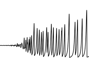
Roll waves result from an instability of free-surface turbulent flows moving down an inclined plane if the slope is greater than some critical value. These waves appear mostly in artificial channels as this critical slope is generally too steep for a natural river. The instability condition was studied by Jeffreys (Reference Jeffreys1925) and Whitham (Reference Whitham1974). This instability is convective in nature, i.e. as a disturbance is transported downstream, it increases in the reference frame moving with the flow, but decreases in the laboratory reference frame. As a result, the phenomenon amplifies a disturbance at the entrance of a channel, while waves gradually grow along the channel. When these waves appear, they eventually break, with the appearance of a succession of turbulent bores and rollers. The development of roll waves is characterized by a coarsening dynamics; some waves overtake waves downstream, which produces even larger waves.
A mathematical discontinuous solution for periodic roll waves was proposed by Dressler (Reference Dressler1949) where continuous profiles described by the Saint-Venant equations are joined by shocks, representing turbulent bores, described by the shock relations. By construction, the length of these shocks is zero. The experiments of Brock (Reference Brock1967, Reference Brock1969, Reference Brock1970) on both natural (i.e. irregular) and periodic roll waves led to the measurement of the growth and the depth profile of roll waves in a laboratory channel. One of the results of this work is that the shock length of roll waves is not negligible and that the amplitude of the waves is overestimated by the theory. Numerical simulations of Brock's experiments were obtained by Zanuttigh & Lamberti (Reference Zanuttigh and Lamberti2002). By introducing a viscous term in the equations, continuous solutions can be obtained (Needham & Merkin Reference Needham and Merkin1984). However, the effect of this term is only to produce a diffuse shock. With a small viscosity, wave amplitudes are still overestimated, as noted by Chang, Demekhin & Kalaidin (Reference Chang, Demekhin and Kalaidin2000) in connection with numerical simulations of Brock's roll wave experiments. As investigated by Hu et al. (Reference Hu, Cao, Hu and Pender2016) in their discussion of the model of Huang & Lee (Reference Huang and Lee2015), the wave amplitude can be reduced to the experimental result with a large viscosity, but then the shock length is greatly overestimated and, in all cases, the model performs poorly with regard to the depth profile. In the framework of the Saint-Venant equations, several mathematical works studied the existence and stability of inviscid or viscous roll waves, and important results were obtained in the near-onset regime (Kranenburg Reference Kranenburg1992; Yu & Kevorkian Reference Yu and Kevorkian1992) and away from onset, with Whitham modulation theory (Whitham Reference Whitham1974), by Tamada & Tougou (Reference Tamada and Tougou1979) and Boudlal & Liapidevskii (Reference Boudlal and Liapidevskii2005). Other stability results were obtained by Katsoulakis & Jin (Reference Katsoulakis and Jin2000) and Noble (Reference Noble2006). A complete stability diagram for the discontinuous roll wave solutions was obtained by Johnson et al. (Reference Johnson, Noble, Rodrigues, Yang and Zumbrun2019).
A new set of equations was obtained in Richard & Gavrilyuk (Reference Richard and Gavrilyuk2012), following an initial work of Teshukov (Reference Teshukov2007), by depth-averaging the Euler equations in the case of shallow flows. Contrary to the assumptions made in deriving the Saint-Venant equations, the fluid velocity is not assumed to be uniform in the depth. The closure of the problem is obtained with the weakly sheared flow assumption. This approach introduces a new variable, called enstrophy because it is related to the square of the vorticity, modelling the variations of the velocity in the depth. The enstrophy is decomposed into two terms, one representing wall shearing, and the other modelling the roller turbulence generated by wave breaking. Periodic roll waves were obtained with this model and compared successfully to Brock's experiments. In particular, the front (or shock) length, the wave amplitude and the depth profiles are in good agreement with the experiments. This work was extended by Ivanova et al. (Reference Ivanova, Gavrilyuk, Nkonga and Richard2017) to the formation and the coarsening of roll waves, with a numerical study of the stability. The performance improvement over the Saint-Venant model is attributable to a more accurate description of the energy balance. It is important to highlight that this approach is based not on the Reynolds-averaged Navier–Stokes equations but on the Euler equations. Consequently, the velocity variations in the depth, and therefore the enstrophy variable, include not only the variations of the mean velocity, but also the turbulent fluctuation. The depth-averaged energy balance equation is one of the equations of the system, and the energy of the system includes an extra term due, in particular, to the turbulence in the roller. The system being hyperbolic, shocks are created in finite time, which are characterized by a creation of enstrophy representing the creation of turbulent energy due to the apparition of a turbulent roller. This turbulent energy decreases by turbulent dissipation, which is modelled in the depth-averaged energy equation. However, there are two parameters in the model, which are calibrated with experimental data. In this respect, an improvement is needed to obtain a truly predictive model. This system was studied from a mathematical point of view by Rodrigues, Yang & Zumbrun (Reference Rodrigues, Yang and Zumbrun2023), who showed that a new type of convective wave can appear in this system, which is not present in the standard Saint-Venant system. Their work showed that the dynamics of this system is much more complex, and their numerical experiments suggest that this model supports time-quasi-periodic solutions, seemingly obtained by superposing convective waves and roll waves.
A completely different approach was followed by Cao et al. (Reference Cao, Hu, Hu, Pender and Liu2015), who used a depth-averaged system based on the Reynolds-averaged Navier–Stokes equations with an eddy viscosity assumption and a  $k$–
$k$– $\epsilon$ turbulence model used by Rastogi & Rodi (Reference Rastogi and Rodi1978). However, as the resulting model performs poorly compared to Brock's experimental data, an empirical term is added to the Reynolds stress, with a coefficient to be calibrated using observed data. This modified model, called SWE-TM, was compared successfully to Brock's experimental results, with good agreement for both natural and periodic roll waves. The SWE-TM is a parabolic system with diffusive terms in the depth-averaged momentum, turbulent kinetic energy and turbulent dissipation balance equations, which are handled with an implicit discretization in the second step of a splitting scheme.
Although their approaches differ in principle, the improvement in roll wave modelling by Richard & Gavrilyuk (Reference Richard and Gavrilyuk2012) and Cao et al. (Reference Cao, Hu, Hu, Pender and Liu2015) over the viscous or inviscid Saint-Venant model was achieved by taking into account the turbulence generated in the wave front.
In a recent work on coastal waves, Kazakova & Richard (Reference Kazakova and Richard2019) derived a model with a structure similar to that of the model of Richard & Gavrilyuk (Reference Richard and Gavrilyuk2012), except that there is no wall friction and shearing, but extended to include dispersive effects, and with a different model for turbulent dissipation, involving only a coefficient of constant value for all breaking waves. We conjecture here that the value of this coefficient is universal for all breaking waves, roll waves or turbulent bores. If this conjecture is valid, then this new form of the dissipative term gives the model a predictive character, since it is no longer necessary to calibrate this parameter on experimental data, thus removing one of the two tunable parameters of the model of Richard & Gavrilyuk (Reference Richard and Gavrilyuk2012). The model of Kazakova & Richard (Reference Kazakova and Richard2019) was extended to the two-dimensional (2-D) case by Richard, Duran & Fabrèges (Reference Richard, Duran and Fabrèges2019) and Duran & Richard (Reference Duran and Richard2020), and validated by comparison to experimental data on shoaling and breaking waves.
The second tunable parameter of the model of Richard & Gavrilyuk (Reference Richard and Gavrilyuk2012) is the value of the wall enstrophy, which was assumed to be transported by the flow and constant in all practical cases. This point was studied in depth by Richard, Couderc & Vila (Reference Richard, Couderc and Vila2023), who derived a 2-D depth-averaged model for open-channel flows down an inclined plane in the smooth turbulent case in the absence of hydraulic jumps, bores or breaking waves. Using a mixing length model of turbulence and a method of matched asymptotic expansions in the outer and inner layers, a three-equation model was derived where the variations in the depth of the mean velocity, in the Reynolds sense, are modelled by an enstrophy variable, similar to the wall enstrophy of the model of Richard & Gavrilyuk (Reference Richard and Gavrilyuk2012). In this new approach, the wall enstrophy is still transported by the flow, but the depth-averaged momentum, energy and enstrophy equations include relaxation source terms with no tunable parameters. The model is determined entirely by the mixing length of the model of Prandtl modified by the damping function of Van Driest (Reference van Driest1956), and thus by the constant  $\kappa$ of von Kármán and the constant $A^{+}$ of van Driest. This mixing length approach is widely recognized as being able to provide an accurate description of open-channel flows over a smooth plane (Nezu & Rodi Reference Nezu and Rodi1986; Cardoso, Graf & Gust Reference Cardoso, Graf and Gust1989). The asymptotic method used by Richard et al. (Reference Richard, Couderc and Vila2023) enables us to calculate consistently the first-order corrections, leading to a system of equations capable of modelling unsteady flows. The model was compared to one-dimensional (1-D) and 2-D experimental measures on unsteady open-channel flows (Yuen Reference Yuen1989; Nezu, Kadota & Nakagawa Reference Nezu, Kadota and Nakagawa1997; Onitsuka & Nezu Reference Onitsuka and Nezu2000; Nezu & Onitsuka Reference Nezu and Onitsuka2002), with good agreement on the reconstructed 2-D and three-dimensional velocity profiles, the bottom shear stress and the flow depth during a flood event.
The aim of this paper is to combine the approach of Kazakova & Richard (Reference Kazakova and Richard2019) for the turbulent dissipation with the model of Richard et al. (Reference Richard, Couderc and Vila2023) for the wall enstrophy, each of which separately removes one of the two tunable parameters of the model of Richard & Gavrilyuk (Reference Richard and Gavrilyuk2012), in order to obtain a fully predictive model for roll waves. Particular attention is paid to the mathematical structure of the resulting model. Section 2 presents the main assumption of this work: the turbulent fluctuation due to the existence of a bottom wall is completely independent of the turbulent fluctuation related to the turbulent roller. This assumption is needed in order to derive the equations that are averaged over the depth in § 3, where the two enstrophies of the model are introduced. The resulting model is a 1-D model that is hyperbolic and solvable by reliable and explicit numerical schemes. As it is validated by comparison with experiments in a channel of finite width, a method to adapt the 1-D-model to a case of a finite width is presented in § 4. The model is validated by comparison with the experimental results obtained by Brock (Reference Brock1967), on periodic roll waves in § 5, and on natural roll waves in § 6.
2. Derivation of the equations
2.1. Assumption of independence between roller and wall turbulence
The model of Richard & Gavrilyuk (Reference Richard and Gavrilyuk2012) is based on the distinction between the vorticity due to the presence of a solid surface at the bottom and the vorticity created in the front of the wave, or between the turbulence due to the bottom wall and the turbulence created in the turbulent roller. This distinction leads to the decomposition of the enstrophy variable into two terms. In the case of roll waves, both types of turbulence coexist.
The modelling of roller turbulence dissipation was improved by Kazakova & Richard (Reference Kazakova and Richard2019) in the case of the related phenomenon of coastal waves. The propagation of these waves is dominated by the dispersive and breaking effects, whereas the wall friction can often be neglected. The depth profiles of breaking waves obtained by this model was validated by comparison with a large range of experiments in various conditions, with very good agreement (Kazakova & Richard Reference Kazakova and Richard2019; Richard et al. Reference Richard, Duran and Fabrèges2019; Duran & Richard Reference Duran and Richard2020). The coefficient in the dissipation term has a universal value for all coastal waves and does not need to be calibrated with experimental data.
On the other hand, only the wall turbulence was taken into account in the hydraulic model of Richard et al. (Reference Richard, Couderc and Vila2023) as the presence of jumps or turbulent rollers was not considered. This led to a model of the bottom shear stress and of the wall friction for unsteady flows, which was also validated by comparison with experiments.
These two approaches led to separate improvements on the two types of turbulence that appear in roll waves, by studying systems where only one of the two types of turbulence is present or considered. The goal now is to superimpose these two descriptions in order to obtain an improved model of roll waves without any tunable coefficients. This implies the formulation of a basic hypothesis, without which the envisaged modelling is impossible, or in any case considerably more complex.
We assume the complete independence between the wall turbulence and the roller turbulence. In Reynolds decomposition, the turbulent fluctuation  $\boldsymbol {v}'$ is decomposed into a wall turbulent fluctuation $\boldsymbol {v}'_W$ and a roller turbulent fluctuation $\boldsymbol {v}'_R$ as
 \begin{equation} \boldsymbol{v}' = \boldsymbol{v}'_W + \boldsymbol{v}'_R. \end{equation}
The flow domain is also decomposed into a roller domain  $\mathcal {D}_R$ for the turbulent roller at the breaking wave fronts, and a wall domain $\mathcal {D}_W$ for the remaining part of the flow (see figure 1). For a point $M$ of the flow, the independence assumption means that $\boldsymbol {v}'_W=\boldsymbol {0}$ if $M \in \mathcal {D}_R$, and $\boldsymbol {v}'_R=\boldsymbol {0}$ if $M \in \mathcal {D}_W$. This assumption of spatial separation automatically implies the independence of the two turbulent fluctuations, i.e. $\overline {\boldsymbol {v}'_W}=0$, $\overline {\boldsymbol {v}'_R}=0$, $\overline {\boldsymbol {v}'_W \boldsymbol {v}'_R}=0$, $\overline {\boldsymbol {v}'_W \otimes \boldsymbol {v}'_R}=0$ and $\overline {\boldsymbol {v}'_R \otimes \boldsymbol {v}'_W}=0$, where the bar denotes the mean value. This assumption leads to a complete decoupling of the two types of turbulence. Interactions exist in reality up to a certain point, but they are assumed to be negligible. The independence assumption simplifies the problem considerably and is sufficient to obtain accurate results. In the following, all equations are defined over the entire domain.

Figure 1. Definition sketch with roller and wall domains.
Similar or stronger assumptions have been made to model wave propagation. The concept of surface rollers proposed for breaking waves by Svendsen (Reference Svendsen1984) and Schäffer, Madsen & Deigaard (Reference Schäffer, Madsen and Deigaard1993) assumes a clear separation between the surface roller, seen as a volume of water carried shorewards with the breaker, and the remaining part of the flow. This hypothesis is implicit in the roll wave model of Richard & Gavrilyuk (Reference Richard and Gavrilyuk2012). In fact, most models of roll waves assume a constant friction coefficient and a constant velocity profile coefficient (often taken equal to 1) in spite of the presence of a surface roller (Kranenburg Reference Kranenburg1992; Zanuttigh & Lamberti Reference Zanuttigh and Lamberti2002; Cao et al. Reference Cao, Hu, Hu, Pender and Liu2015). This implies that the effect of the roller on the wall flow and on the mean velocity profile is neglected. In essence, this is the same assumption as the independence assumption above, since this assumption allows us to treat bottom friction and roller turbulence separately. The validity of this very common assumption is due to the fact that the two effects are spatially quite well separated, one being due to the bottom wall of the flow, and the other occurring rather on the free surface side of the front part of the waves.
2.2. Method of derivation
The flow is assumed to be turbulent with a Reynolds number large enough to be able to neglect viscous effects, except close to the wall or for the turbulent dissipation. Similarly, all surface tension effects are also neglected.
The method used in Richard et al. (Reference Richard, Couderc and Vila2023) to handle the wall turbulence is based on the Reynolds equations, where the Reynolds stresses are modelled with an eddy viscosity hypothesis calculated with the mixing length model. In the resulting equations, which are then averaged over the depth, the velocity is the mean velocity in the Reynolds sense. Therefore, the variations of the velocity with depth represent not turbulent fluctuations, but variations of the mean velocity, which we call shear. This effect is called dispersion by Cao et al. (Reference Cao, Hu, Hu, Pender and Liu2015), but we do not use this term to avoid confusion with the dispersive effects that appear in some hydraulic models, such as the Serre–Green–Naghdi model, used in particular to model coastal waves or undular bores. In this method, asymptotic expansions are used to derive consistent expressions of the shear stress at the bottom and of the dissipation due to the eddy viscosity.
The approach used by Richard & Gavrilyuk (Reference Richard and Gavrilyuk2012) to model roller turbulence is wholly different since the basic equations are the Euler equations, which implies that the turbulence is resolved, even if it is in a depth-averaged way. Consequently, the variations of velocity in the depth include not only the variations of the mean velocity, but also the turbulent fluctuations. The roller turbulence, quantified by the roller enstrophy, is created by the shocks produced by this hyperbolic system. In the model of Kazakova & Richard (Reference Kazakova and Richard2019), because of the dispersive effects, the system is not hyperbolic. The chosen approach was different and used a filtering operation, as in the large-eddy simulation, to decompose the velocity into a resolved component representing the large-scale turbulence and a residual component for the small-scale turbulence. The residual-stress tensor was modelled by an eddy viscosity assumption, and the filtered velocity was averaged over the depth. Therefore, the variations of this velocity in the depth, taken into account in the model by the enstrophy, includes the large-scale turbulence of breaking waves. The turbulence and enstrophy are created by viscous terms due to the residual motions. In the cases of both Richard & Gavrilyuk (Reference Richard and Gavrilyuk2012) and Kazakova & Richard (Reference Kazakova and Richard2019), the turbulent dissipation was modelled using depth-averaged model quantities, but not in the same way. The model chosen by Kazakova & Richard (Reference Kazakova and Richard2019) is preferable, because it involves a dimensionless coefficient whose value is constant and does not need to be calibrated with experimental data. On the other hand, diffusion terms due to the molecular viscosity were neglected in both approaches since this diffusion is not negligible only close to a wall (Pope Reference Pope2000), which is not the case for the turbulence of rollers or breaking waves. In the present paper, since dispersive effects are not taken into account, the filtering operation is not necessary since the final model is expected to be hyperbolic and able to create turbulence, i.e. roller enstrophy, by the shocks, exactly as in the model of Richard & Gavrilyuk (Reference Richard and Gavrilyuk2012).
The problem to be solved, in order to superimpose the two models of Richard et al. (Reference Richard, Couderc and Vila2023) and Kazakova & Richard (Reference Kazakova and Richard2019), is therefore to reconcile two different approaches, the first based on Reynolds averaging, and the other not. The independence assumption makes it easy to superimpose these two approaches. In particular, the asymptotic expansions of Richard et al. (Reference Richard, Couderc and Vila2023), used to express bottom friction, are not modified, thanks to this assumption, by the possible existence of a turbulent roller.
2.3. Mass conservation
Reynolds decomposition for the velocity field is written as  $\boldsymbol {v}= \bar {\boldsymbol {v}} +\boldsymbol {v}'_W+\boldsymbol {v}'_R$, denoting by $\bar {\boldsymbol {v}}$ the mean velocity, and using the separation (2.1) between wall turbulence fluctuation and roller turbulence fluctuation. The incompressibility assumption implies $\mathrm {div}\, \boldsymbol {v}=0$, which entails that, separately, $\mathrm {div}\, \bar {\boldsymbol {v}}=0$ and $\mathrm {div}\, \boldsymbol {v}'=0$. The independence assumption leads to $\mathrm {div}\, \boldsymbol {v}'_W=0$ and $\mathrm {div}\, \boldsymbol {v}'_R=0$.
2.4. Momentum balance equation
In the Reynolds equations, the decoupling between wall and roller contributions can be applied to the Reynolds stress, since the independence assumption gives  $\overline {\boldsymbol {v}'_W \otimes \boldsymbol {v}'_R}=\overline { \boldsymbol {v}'_W} \otimes \overline { \boldsymbol {v}'_R}=0$ and $\overline { \boldsymbol {v}'_R \otimes \boldsymbol {v}'_W}=\overline { \boldsymbol {v}'_R} \otimes \overline { \boldsymbol {v}'_W}=0$. This yields $\overline { \boldsymbol {v}' \otimes \boldsymbol {v}'} = \overline {\boldsymbol {v}'_W \otimes \boldsymbol {v}'_W} +\, \overline {\boldsymbol {v}'_R \otimes \boldsymbol {v}'_R}$. The wall contribution is handled with a turbulent viscosity hypothesis, which can be written as
 \begin{equation} - \overline{\boldsymbol{v}'_W\otimes \boldsymbol{v}'_W} ={-} \tfrac{2}{3}\,k_W \boldsymbol{\mathsf{I}}+ 2 \nu_{T} \overline{\boldsymbol{\mathsf{D}}}, \end{equation}
where  $k_W$ is the turbulent kinetic energy associated with the wall turbulence defined by $k_W = \overline {\boldsymbol {v}'_W\boldsymbol {\cdot } \boldsymbol {v}'_W}/2$, $\boldsymbol{\mathsf{I}}$ is the identity tensor, $\nu _{T}$ is the eddy viscosity of the wall turbulence, and $\overline{\boldsymbol{\mathsf{D}}}$ is the mean rate-of-strain tensor. Denoting by $\boldsymbol {g}$ the gravity acceleration, by $p$ the pressure, and by $\rho$ the fluid density (the fluid is water), and defining the modified pressure
 \begin{equation} p^{{\ast}}= p + \tfrac{2}{3}\rho k_W,\quad \overline{p^{{\ast}}}= \overline p + \tfrac{2}{3}\rho k_W, \end{equation}
the Reynolds equation can be written as
 \begin{equation} \frac{\partial \bar{v}}{\partial t} + \mathbf{div}\left(\overline{\boldsymbol{v}_R\otimes \boldsymbol{v}_R}+\frac{\overline{p^{{\ast}}}}{\rho}\,\boldsymbol{\mathsf{I}}\right) = \boldsymbol{g}+\mathbf{div}(2 \nu_{eff} \overline{\boldsymbol{\mathsf{D}}}), \end{equation}
 where the velocity  $\boldsymbol {v}_R$ is defined by
 \begin{equation} \boldsymbol{v}_R = \bar{\boldsymbol{v}} + \boldsymbol{v}'_R, \end{equation}
and the effective kinematic viscosity is  $\nu _{eff}=\nu _{T} + \nu$, with $\nu$ denoting the molecular kinematic viscosity. In practice, the term due to the molecular viscosity is negligible except in the viscous wall layer. This term appears only in the asymptotic expansions in the inner layer, and it influences the model only through the asymptotic matching procedure (Richard et al. Reference Richard, Couderc and Vila2023). Equation (2.4) can be rewritten as
 \begin{equation} \frac{\partial \bar{v}}{\partial t} + \mathbf{div}\left(\overline{\boldsymbol{v}_R\otimes \boldsymbol{v}_R}+\frac{\bar{p}}{\rho}\,\boldsymbol{\mathsf{I}}\right) = \boldsymbol{g}-\mathbf{div}( \overline{\boldsymbol{v}'_W\otimes \boldsymbol{v}'_W}) +\mathbf{div}(2 \nu \overline{\boldsymbol{\mathsf{D}}}). \end{equation}
Denoting by  $\boldsymbol{\mathsf{D}}$, the strain-rate tensor, (2.6) is subtracted from the Navier–Stokes equation
 \begin{equation} \frac{\partial \boldsymbol{v}}{\partial t} + \mathbf{div}\left( \boldsymbol{v} \otimes \boldsymbol{v} +\frac{p}{\rho}\,\boldsymbol{\mathsf{I}} \right) = \boldsymbol{g}+ \mathbf{div}(2 \nu \boldsymbol{\mathsf{D}}) \end{equation}
to obtain the equation for the fluctuating velocity
 \begin{equation} \frac{\partial \boldsymbol{v}'}{\partial t} + \mathbf{div}\left( \boldsymbol{v} \otimes \boldsymbol{v} - \overline{\boldsymbol{v}_R\otimes \boldsymbol{v}_R} + \frac{p'}{\rho}\,\boldsymbol{\mathsf{I}}\right) = \mathbf{div}(\overline{\boldsymbol{v}'_W\otimes \boldsymbol{v}'_W}) + \mathbf{div}(2\nu \boldsymbol{\mathsf{D}}' ) ,\end{equation}
where  $p'=p-\bar {p}$ is the fluctuating pressure, and $\boldsymbol{\mathsf{D}}'=\boldsymbol{\mathsf{D}}-\overline{\boldsymbol{\mathsf{D}}}$. The decomposition (2.1) is extended to the fluctuating pressure, writing $p'=p'_R$ if $M \in \mathcal {D}_R$, and $p'=p'_W$ if $M \in \mathcal {D}_W$. In the same way, $\boldsymbol{\mathsf{D}}'=\boldsymbol{\mathsf{D}}'_W + \boldsymbol{\mathsf{D}}'_R$. The roller turbulence can be completely decoupled from the wall turbulence, since $\boldsymbol {v}'_W=0$, $\boldsymbol{\mathsf{D}}'_W=0$ and $p'_W=0$ in the roller domain $\mathcal {D}_R$, and $\boldsymbol {v}'_R=0$, $\boldsymbol{\mathsf{D}}'_R=0$ and $p'_R=0$ in the wall domain $\mathcal {D}_W$. Therefore, $\boldsymbol {v}'_R \otimes \boldsymbol {v}'_W = \boldsymbol {v}'_W \otimes \boldsymbol {v}'_R=\boldsymbol {0}$ and the roller fluctuation velocity evolves by
 \begin{equation} \frac{\partial \boldsymbol{v}'_R}{\partial t} + \mathbf{div}\left( \boldsymbol{v}_R \otimes \boldsymbol{v}_R - \overline{\boldsymbol{v}_R\otimes \boldsymbol{v}_R} + \frac{p'_R}{\rho}\,\boldsymbol{\mathsf{I}}\right) = \mathbf{div}(2\nu \boldsymbol{\mathsf{D}}'_R). \end{equation}
Defining  $p_R = \bar {p}+p'_R$, $p^{\ast }_R=p_R+(2/3)\rho k_W$ and $\boldsymbol{\mathsf{D}}_R = \overline{\boldsymbol{\mathsf{D}}}+\boldsymbol{\mathsf{D}}'_R$, the addition of (2.9) to (2.4) gives
 \begin{equation} \frac{\partial \boldsymbol{v}_R}{\partial t} + \mathbf{div}\left( \boldsymbol{v}_R \otimes \boldsymbol{v}_R +\frac{p^{{\ast}}_R}{\rho}\,\boldsymbol{\mathsf{I}} \right) = \boldsymbol{g}+ \mathbf{div}(2 \nu_{T} \overline{\boldsymbol{\mathsf{D}}} ) + \mathbf{div}(2 \nu \boldsymbol{\mathsf{D}}_R ). \end{equation}
In the wall domain  $\mathcal {D}_W$, $\boldsymbol {v}_R = \bar {\boldsymbol {v}}$, $\boldsymbol{\mathsf{D}}_R = \overline{\boldsymbol{\mathsf{D}}}$, $p^{\ast }_R=\overline {p^{\ast }}$, and this equation simply reduces to (2.4). In the roller domain, $k_W=0$ and $p^{\ast }_R=\bar {p}+p'_R$. With the independence assumption between roller and wall turbulences, the momentum balance equation is similar to the Navier–Stokes equation except that the velocity field $\boldsymbol {v}_R$ and the special pressure field $p^{\ast }_R$ are used instead of the usual velocity and pressure, and there is an extra diffusive term due to the eddy viscosity $\nu _{T}$ modelling the wall turbulence. The diffusive term due to the molecular viscosity is negligible except close to the wall.
2.5. Energy balance equation
Since the energy balance equation is one of the basic equations of the depth-averaged model, the same method is applied to the energy equation. The equation for the kinetic energy of the mean flow can be written as
 \begin{align} \frac{\partial }{\partial t}\left(\frac{\bar{\boldsymbol{v}} \boldsymbol{\cdot} \bar{\boldsymbol{v}}}{2}\right) + \mathrm{div}\left(\frac{\bar{\boldsymbol{v}} \boldsymbol{\cdot} \bar{\boldsymbol{v}}}{2}\,\bar{\boldsymbol{v}} + \frac{\bar{p}}{\rho}\,\bar{\boldsymbol{v}} + \bar{\boldsymbol{v}} \boldsymbol{\cdot} \overline{\boldsymbol{v}' \otimes \boldsymbol{v}'} - 2 \nu \bar{\boldsymbol{v}} \boldsymbol{\cdot} \overline{\boldsymbol{\mathsf{D}}}\right) = \overline{\boldsymbol{v}' \otimes \boldsymbol{v}'}:\mathbf{grad} \,\bar{\boldsymbol{v}} + \boldsymbol{g} \boldsymbol{\cdot} \bar{\boldsymbol{v}} - \bar{\epsilon}, \end{align}
where  $\bar {\epsilon } = 2 \nu \overline{\boldsymbol{\mathsf{D}}} : \overline{\boldsymbol{\mathsf{D}}}$ is the dissipation due to the mean flow, which is negligible for high Reynolds numbers, as is the diffusive term due to the molecular viscosity. From the evolution equation (2.8) of the fluctuating velocity, we can obtain the equation
 \begin{align} &\frac{\partial }{\partial t}\left(\frac{\boldsymbol{v}' \boldsymbol{\cdot} \boldsymbol{v}'}{2}\right) + \mathrm{div}\left(\frac{\boldsymbol{v}' \boldsymbol{\cdot} \boldsymbol{v}'}{2}\,\bar{\boldsymbol{v}} + \frac{p'}{\rho}\,\boldsymbol{v}' +\frac{ \boldsymbol{v}'}{2} \boldsymbol{\cdot} \boldsymbol{v}' \otimes \boldsymbol{v}' - 2 \nu \boldsymbol{v}' \boldsymbol{\cdot} \boldsymbol{\mathsf{D}}'\right)\nonumber\\ &\quad ={-}\boldsymbol{v}' \otimes \boldsymbol{v}':\mathbf{grad} \,\bar{\boldsymbol{v}} + \boldsymbol{v}' \boldsymbol{\cdot} \mathbf{div} (\overline{ \boldsymbol{v}' \otimes \boldsymbol{v}'} ) - 2 \nu \boldsymbol{\mathsf{D}}' : \boldsymbol{\mathsf{D}}'. \end{align}
Taking the mean of this equation gives the equation for the turbulent kinetic energy. The mean of the first term on the right-hand side of (2.12) is usually called the production, and  $2\nu \overline {\boldsymbol{\mathsf{D}}' : \boldsymbol{\mathsf{D}}'}$ is the dissipation of turbulent kinetic energy, usually denoted by $\epsilon$. The mean of the second term on the right-hand side of (2.12) is zero. The same decoupling procedure as for the mass and momentum balance equations is used for (2.12) and leads to
 \begin{align} &\frac{\partial }{\partial
t}\left(\frac{\boldsymbol{v}'_R
\boldsymbol{\cdot} \boldsymbol{v}'_R}{2}\right) +
\mathrm{div}\left(\frac{\boldsymbol{v}'_R \boldsymbol{\cdot}
\boldsymbol{v}'_R}{2}\,\bar{\boldsymbol{v}} +
\frac{p'_R}{\rho}\,\boldsymbol{v}'_R
+\frac{ \boldsymbol{v}'_R}{2} \boldsymbol{\cdot}
\boldsymbol{v}'_R \otimes
\boldsymbol{v}'_R - 2 \nu
\boldsymbol{v}'_R \boldsymbol{\cdot}
\boldsymbol{\mathsf{D}}'_R\right)\nonumber\\ &\quad
={-}\boldsymbol{v}'_R \otimes
\boldsymbol{v}'_R:\mathbf{grad}
\,\bar{\boldsymbol{v}} + \boldsymbol{v}'_R \boldsymbol{\cdot}
\mathbf{div} (\overline{ \boldsymbol{v}'_R \otimes
\boldsymbol{v}'_R} ) - 2 \nu
\boldsymbol{\mathsf{D}}'_R : \boldsymbol{\mathsf{D}}'_R.
\end{align}
\begin{align} &\frac{\partial }{\partial
t}\left(\frac{\boldsymbol{v}'_R
\boldsymbol{\cdot} \boldsymbol{v}'_R}{2}\right) +
\mathrm{div}\left(\frac{\boldsymbol{v}'_R \boldsymbol{\cdot}
\boldsymbol{v}'_R}{2}\,\bar{\boldsymbol{v}} +
\frac{p'_R}{\rho}\,\boldsymbol{v}'_R
+\frac{ \boldsymbol{v}'_R}{2} \boldsymbol{\cdot}
\boldsymbol{v}'_R \otimes
\boldsymbol{v}'_R - 2 \nu
\boldsymbol{v}'_R \boldsymbol{\cdot}
\boldsymbol{\mathsf{D}}'_R\right)\nonumber\\ &\quad
={-}\boldsymbol{v}'_R \otimes
\boldsymbol{v}'_R:\mathbf{grad}
\,\bar{\boldsymbol{v}} + \boldsymbol{v}'_R \boldsymbol{\cdot}
\mathbf{div} (\overline{ \boldsymbol{v}'_R \otimes
\boldsymbol{v}'_R} ) - 2 \nu
\boldsymbol{\mathsf{D}}'_R : \boldsymbol{\mathsf{D}}'_R.
\end{align}
Forming the sum  $\text {(\ref {eqn11})} + \text {\eqref {eqn13}} + \bar {\boldsymbol {v}}\boldsymbol {\cdot } \text {(\ref {eqn9})} + \boldsymbol {v}'_R\boldsymbol {\cdot } \text {(\ref {eqn4})}$ gives
 \begin{align} &\frac{\partial}{\partial t}\left(\frac{\boldsymbol{v}_R\boldsymbol{\cdot}\boldsymbol{v}_R}{2}\right) + \mathrm{div}\left[\left(\frac{\boldsymbol{v}_R\boldsymbol{\cdot}\boldsymbol{v}_R}{2}+\frac{p^{{\ast}}_R}{\rho}\right)\boldsymbol{v}_R \right]\nonumber\\ &\quad =\boldsymbol{g} \boldsymbol{\cdot} \boldsymbol{v}_R + \mathrm{div}( 2 \nu_{T} \boldsymbol{v}_R\boldsymbol{\cdot} \overline{\boldsymbol{\mathsf{D}}})-2\nu_{T} \overline{\boldsymbol{\mathsf{D}}}:\boldsymbol{\mathsf{D}}_R - 2 \nu \boldsymbol{\mathsf{D}}'_R : \boldsymbol{\mathsf{D}}'_R, \end{align}
where the negligible terms involving the molecular viscosity have been removed. The last term on the right-hand side of (2.14) is the only term with  $\nu$, which is not negligible because it takes into account the dissipation due to roller turbulence. This equation is similar to the energy balance equation associated with the Navier–Stokes equations with the velocity field $\boldsymbol {v}_R$ and the pressure $p^{\ast }_R$, as well as diffusive and dissipative terms due to the eddy viscosity related to the wall turbulence.
3. Depth-averaged equations
3.1. Shear and roller enstrophies
The mass conservation equation for the velocity field  $\boldsymbol {v}_R$ can be written as $\mathrm {div}\, \boldsymbol {v}_R=0$. This equation, the momentum balance equation (2.10) and the energy equation (2.14) are averaged over the depth. For any quantity $A$, the depth-averaged quantity is defined as
 \begin{equation} \langle A \rangle = \frac{1}{h}\int_0^h A\, \mathrm{d}z, \end{equation}
where  $h$ is the fluid depth. The free-surface location can be written as the sum of a Reynolds-averaged term and a turbulent fluctuation. However, the contribution of the fluctuation of the free surface for depth-averaged models is negligible, as explained by Svendsen et al. (Reference Svendsen, Veeramony, Bakunin and Kirby2000) for turbulent hydraulic jumps, and by Stansby & Feng (Reference Stansby and Feng2005) with measurements on surf zone waves. The fluid depth $h$ can thus be seen as a Reynolds-averaged quantity, and the usual boundary conditions can be used. Further discussion of this issue can be found in Kazakova & Richard (Reference Kazakova and Richard2019).
The flow is assumed to be 2-D in order to derive a 1-D depth-averaged model. The coordinates  $x$ and $z$, and the inclination angle $\theta$, are defined in figure 1. The components of $\boldsymbol {v}_R$ are $u$ and $w$ in the $Ox$ and $Oz$ directions, respectively. To lighten the notations, the average of the velocity $u$ over the depth is denoted by $U$, i.e. $U= \langle u \rangle$. The velocity is decomposed as the sum of its depth-averaged value and a deviation $u^{\ast }$ as $u=U+u^{\ast }$ (Teshukov Reference Teshukov2007; Richard & Gavrilyuk Reference Richard and Gavrilyuk2012; Kazakova & Richard Reference Kazakova and Richard2019; Richard et al. Reference Richard, Couderc and Vila2023). This deviation is in turn decomposed into a shear contribution $u^{\ast }_s$, due to the variation in $\mathcal {D}_W$ of the mean velocity with the depth, and a roller contribution $u^{\ast }_r$, due to the roller turbulence in $\mathcal {D}_R$, as $u^{\ast } = u^{\ast }_s + u^{\ast }_r$. These two contributions are assumed to be independent, i.e. $\langle u^{\ast }_s \rangle = \langle u^{\ast }_r \rangle = 0$ and $\langle u^{\ast }_s u^{\ast }_r \rangle = 0$. These two contributions to the deviations correspond to two enstrophies defined as
 \begin{equation} \psi = \frac{\langle u^{{\ast} 2}_s \rangle }{h^2}, \quad \varphi = \frac{\langle u^{{\ast} 2}_r \rangle }{h^2}. \end{equation}
The enstrophy  $\psi$ is called shear enstrophy, and $\varphi$ is the roller enstrophy. Therefore, the average of the square of the velocity can be written as $\langle u^2 \rangle = U^2 + h^2 \psi + h^2 \varphi$.
3.2. The shallow-water assumption and the Teshukov approximation
The equations of mass, momentum and energy are supplemented by the boundary conditions. The no-penetration condition at the bottom can be written as  $w(0)=0$, while the kinematic condition at the free surface is $w(h) = \partial h / \partial t + u(h)\,\partial h / \partial x$. The dynamic boundary condition at the free surface can be written as $(\boldsymbol {\sigma }\boldsymbol {\cdot } \boldsymbol {n})(h) = 0$, where $\boldsymbol {\sigma }$ is the Cauchy stress tensor, and $\boldsymbol {n}$ is the unit normal vector at the free surface. This boundary condition is detailed in Kazakova & Richard (Reference Kazakova and Richard2019).
Averaging over the depth, the mass conservation gives
 \begin{equation} \frac{\partial h}{\partial t} + \frac{\partial hU}{\partial x}=0, \end{equation}
without any approximation. On the contrary, several assumptions are needed for the derivation of the depth-averaged momentum and energy balance equations. The first assumption is the usual shallow-water approximation: the fluid depth, characterized by  $h_0$, is assumed to be small compared to a characteristic length $L$ of variation of the flow variables in the $Ox$ direction. The ratio $h_0 / L$ defines a small parameter $\varepsilon = h_0/L \ll 1$, which is the basis for the implementation of an asymptotic method. Defining the stress tensor $\boldsymbol {\tau }^W = 2 \nu _T \overline{\boldsymbol{\mathsf{D}}}$ related to the eddy viscosity and the wall turbulence, the shallow-water scaling scaling used in Richard et al. (Reference Richard, Couderc and Vila2023) implies that the normal stresses $\tau ^W_{xx}$ and $\tau ^W_{zz}$ are small compared with the shear stress $\tau ^W_{xz}$, i.e. $\tau ^W_{xx}/\tau ^W_{xz}=O(\varepsilon )$. Another assumption is that the molecular viscosity is very small compared with a characteristic eddy viscosity. This implies that the Reynolds number, defined with the molecular viscosity, is larger than $O(\varepsilon ^{-2})$ (Richard et al. Reference Richard, Couderc and Vila2023). All terms with the molecular viscosity are therefore negligible in the momentum and energy equations, except the dissipation due to roller turbulence.
The momentum balance equation (2.10) in the  $Oz$ direction gives the pressure. Neglecting terms of $O(\varepsilon )$ due to the stress tensor $\boldsymbol {\tau }^W$, and terms of $O(\varepsilon ^2)$ due to the vertical fluid acceleration, the pressure is hydrostatic. Using the boundary conditions, depth-averaging the momentum balance equation (2.10) in the $Ox$ direction leads to
 \begin{equation} \frac{\partial hU}{\partial t} + \frac{\partial}{\partial x}( hU^2 +\varPi ) = gh\sin \theta - \frac{\tau^W_{xz}(0)}{\rho}, \end{equation}
where
 \begin{equation} \varPi = h^3\psi + h^3 \varphi + \frac{gh^2}{2}\cos \theta. \end{equation}
The same averaging procedure for the energy equation (2.14) gives
 \begin{equation} \frac{\partial he}{\partial t} + \frac{\partial}{\partial x}\left(hUe+\varPi U + \frac{h}{2}\,\langle u^{{\ast} 3}_s \rangle + \frac{h}{2}\,\langle u^{{\ast} 3}_r \rangle \right)=ghU \sin \theta - W_s - W_r, \end{equation}
where the energy is
 \begin{equation} e = \frac{U^2}{2}+\frac{h^2\psi}{2}+\frac{h^2\varphi}{2}+\frac{gh}{2}\cos \theta, \end{equation}
and the shear and roller dissipation are respectively
 \begin{equation}
W_s=\int_0^h 2 \nu_T \overline{\boldsymbol{\mathsf{D}}}:\overline{\boldsymbol{\mathsf{D}}}\, \mathrm{d}z, \quad W_r = \int_0^h 2 \nu
\boldsymbol{\mathsf{D}}'_R:\boldsymbol{\mathsf{D}}'_R \,
\mathrm{d}z.
\end{equation}
\begin{equation}
W_s=\int_0^h 2 \nu_T \overline{\boldsymbol{\mathsf{D}}}:\overline{\boldsymbol{\mathsf{D}}}\, \mathrm{d}z, \quad W_r = \int_0^h 2 \nu
\boldsymbol{\mathsf{D}}'_R:\boldsymbol{\mathsf{D}}'_R \,
\mathrm{d}z.
\end{equation}
The concept of weakly sheared flows was introduced by Teshukov (Reference Teshukov2007). In the context of this paper, this is more properly an assumption of a weakly turbulent flow; the ratio of the roller turbulent deviation  $u^{\ast }_R$ to the depth-averaged velocity $U$ is supposed to be of $O(\varepsilon ^\beta )$. The term $h^3 \varphi$ in the expression (3.5) of $\varPi$ in the momentum flux of (3.4) and in the energy flux of (3.6) are of $O(\varepsilon ^{2\beta })$, and the term with $\langle u^{\ast 3}_r \rangle$ is of $O(\varepsilon ^{3\beta })$. This assumption allows us to neglect the term with $\langle u^{\ast 3}_r \rangle$ in the energy equation (3.6) provided that $\beta >0$. In Teshukov (Reference Teshukov2007) and Richard & Gavrilyuk (Reference Richard and Gavrilyuk2012), the enstrophy term in (3.4) is kept, while the non-hydrostatic correction to the pressure, which is due to the vertical acceleration and which is of $O(\varepsilon ^2)$, is neglected. This implies that $\beta$ must also satisfy the condition $\beta <1$. In this paper, terms of $O(\varepsilon )$ are also neglected in the pressure, which implies the condition $\beta < 1/2$. Finally, the condition on $\beta$ for the derivation to be consistent is $0 < \beta < 1/2$.
A similar approximation was obtained by Richard et al. (Reference Richard, Couderc and Vila2023) for the shear deviation using the small parameter  $\mu = 2 \ln ^{-1} (\kappa ^2\,Re)$, where $\kappa$ is the von Kármán constant, and $Re=hU/\nu$ is the Reynolds number. The shear deviation $u^{\ast }_s$ is of $O(\mu )$, while the terms with the shear enstrophy $\psi$ in (3.4) and (3.6) are of $O(\mu ^2)$, and the term with $\langle u^{\ast 3}_s \rangle$ is of $O(\mu ^3)$. While $\varepsilon$ is the main small parameter, $\mu$ is treated as a second small parameter, with $\varepsilon < \mu <1$, and terms of $O(\mu ^3)$ can be neglected. A similar approximation was used by Luchini & Charru (Reference Luchini and Charru2010), who used the small parameter $u_b / U$ introduced by Mellor (Reference Mellor1972), where $u_b$ is the shear or friction velocity. This small parameter plays the same role as $\mu$ and allowed the authors to keep terms of the order of $(u_b / U)^2$ and to neglect terms of the order of $(u_b / U)^3$. This approximation is equivalent to Teshukov's assumption in the sense that the mean of the cube of the deviation can be neglected consistently in the energy balance equation.
In fact, since the average of the deviation is zero, the deviation is negative for some values of  $z$, and positive for others. The same applies to the cube of the deviation, which means that the average of the cube of the deviation is smaller than its order of magnitude would suggest. For example, if the velocity were a linear function of the depth, then the average of the cube of the deviation would be zero. However, this is not the case for the enstrophy, which depends on the square of the deviation, which is of course always positive. Consequently, neglecting the average of the cube of the deviation in front of the average of the square has a greater validity than predicted by the orders of magnitude of the asymptotic developments. The Teshukov approximation and equivalent approximations therefore have a wider validity. In particular, it is possible to describe, within the framework of this approximation, flows for which turbulence is not precisely weak, such as highly turbulent hydraulic jumps (Richard & Gavrilyuk Reference Richard and Gavrilyuk2013).
3.3. Expressions for wall friction and dissipation
The flow is assumed to be in the smooth turbulent case. This assumption is valid if  $Re^{\ast }=v^{\ast }k_s/\nu <4$, where $Re^{\ast }$ is the shear Reynolds number, $v^{\ast }$ is the shear velocity, and $k_s$ is the average surface roughness (Henderson Reference Henderson1966; Chanson Reference Chanson2004). The assumption of independence between roller and wall turbulence enables us to use the asymptotic expansions of Richard et al. (Reference Richard, Couderc and Vila2023) obtained in the smooth turbulent case. Each variable is expanded with respect to the small parameter $\varepsilon$. By inserting these expansions into the equations of the system, the terms of order 0 ( $O(1)$) and then of order 1 ( $O(\varepsilon )$) are obtained for each variable. It is then possible to express the shear stress at the bottom $\tau ^W_{xz}(0)$ and the shear dissipation $W_s$ as relaxation source terms for $U$ and $\psi$. These expressions are (Richard et al. Reference Richard, Couderc and Vila2023)
 $$\begin{gather} \frac{\tau^W_{xz}(0)}{\rho}=C_f U\,|U| - \frac{\alpha_1}{\kappa}\sqrt{C_f}\,(C_f U\,|U| - \hat gh ) - (\alpha_2 \kappa -\alpha \alpha_1 \sqrt{C_f})\sqrt{C_f}\,h\left(h\psi - \frac{\hat g }{\kappa^2}\right), \end{gather}$$
 $$\begin{gather}W_s = C_f U^2\,|U| - \frac{\alpha}{\kappa}\,\sqrt{C_f}\,(C_f U\,|U| - \hat{g}h )U + \alpha^2hC_f \left(h\psi - \frac{\hat{g}}{\kappa^2}\right)U, \end{gather}$$
where  $\hat {g}=g \sin \theta$, $\alpha =R_1 - R +1$, $\alpha _2 = [2(\zeta (3) - 1)]^{-1} \simeq 2.47$, $\alpha _1 = \alpha - \alpha _2$, and the friction coefficient is obtained consistently with the explicit relation
 \begin{equation} C_f = \kappa^2 \left(R-2+2 \ln 2 + \ln \kappa + \ln \frac{\sqrt{\hat{g}h^3}}{\nu}\right)^{{-}2}. \end{equation}
In the above expressions,  $\zeta$ is the Riemann zeta function, $\zeta (3) \simeq 1.20$, and the functions $R$ and $R_1$ are given by
 $$\begin{gather} R= \int_0^\infty \frac{\mathrm{d}\xi}{1+\sqrt{1+\xi^2(1-\mathrm{e}^{-\xi/A})^2}}-\int_0^\infty \frac{\mathrm{d}\xi}{1+\sqrt{1+\xi^2}}, \end{gather}$$
 $$\begin{gather}R_1= \int_0^\infty \frac{\mathrm{d}\xi}{\sqrt{1+\xi^2(1-\mathrm{e}^{-\xi/A})^2}}-\int_0^\infty \frac{\mathrm{d}\xi}{\sqrt{1+\xi^2}}, \end{gather}$$
where  $A=2\kappa A^+$. Full details of how these functions are obtained are given in Richard et al. (Reference Richard, Couderc and Vila2023). Once the von Kármán constant $\kappa$ and the constant $A^+$ of the van Driest damping function are fixed, all parameters of the model are known.
The roller dissipation is modelled as in Kazakova & Richard (Reference Kazakova and Richard2019) as
 \begin{equation} W_r = \frac{C_r}{2}\,h^3 \varphi^{3/2}. \end{equation}
The coefficient  $C_r$ has the universal value $C_r = 0.48$, which was validated by comparison with a large number of experiments on breaking waves in a wide range of conditions in Kazakova & Richard (Reference Kazakova and Richard2019), Richard et al. (Reference Richard, Duran and Fabrèges2019) and Duran & Richard (Reference Duran and Richard2020). This expression is similar to the expression for the turbulent dissipation in the turbulent kinetic energy model, where the turbulent dissipation $\epsilon$ is based on the turbulent kinetic energy $k$ and on the mixing length $l_m$, and written as $\epsilon =C_D k^{3/2}/l_m$, with a dimensionless constant $C_D$ (Pope Reference Pope2000). In the present model, the mixing length is replaced by the depth $h$, the turbulent kinetic energy has the dimensions of $h^2 \varphi$, and $W_r$ is a depth-integrated quantity. As in the study of turbulent flows, the expression of the roller dissipation does not depend on the viscosity. This is usually explained by the energy cascade and the hypotheses of Kolmogorov. The rate of dissipation is determined by the transfer of energy from the largest eddies, independently of the viscosity, even if the energy is dissipated at the smallest scales by viscous action (Pope Reference Pope2000).
3.4. Conservation of energy and shear enstrophy
From the mass, momentum and energy equations, an evolution equation for the total enstrophy  $\psi + \varphi$ can be obtained. This equation can be written as
 \begin{align} &\frac{\partial h (\psi + \varphi )}{\partial t}+\frac{\partial hU(\psi+\varphi )}{\partial x}\nonumber\\ &\quad =2\,\frac{\alpha_2}{\kappa}\,\frac{\sqrt{C_f}}{h^2}\,U (C_f U\,|U| -\hat{g}h ) - 2\alpha_2 (\kappa + \alpha \sqrt{C_f})\, \frac{\sqrt{C_f}}{h}\,U \left(h\psi - \frac{\hat{g}}{\kappa^2}\right)- C_r h \varphi^{3/2}. \end{align}
The equations for  $\psi$ and $\varphi$ can be decoupled thanks to the independency assumption. The balance equation for the shear enstrophy derived in Richard et al. (Reference Richard, Couderc and Vila2023) is thus recovered. This equation is
 \begin{align} \frac{\partial h \psi}{\partial t}+\frac{\partial hU\psi}{\partial x}=2\,\frac{\alpha_2}{\kappa}\,\frac{\sqrt{C_f}}{h^2}\,U (C_f U\,|U| -\hat{g}h ) - 2\alpha_2 (\kappa + \alpha \sqrt{C_f})\,\frac{\sqrt{C_f}}{h}\,U \left(h\psi - \frac{\hat{g}}{\kappa^2}\right). \end{align}
Consequently, the equation for the roller enstrophy can be written as
 \begin{equation} \frac{\partial h \varphi}{\partial t}+ \frac{\partial hU\varphi}{\partial x}={-} C_r h \varphi^{3/2}. \end{equation}
The resulting model is hyperbolic and therefore creates shocks in finite time. From a physical point of view, the appearance of a shock models the breaking of the wave and the creation of roller turbulence.
In the case of the Saint-Venant system of equations (or nonlinear shallow-water equations), the two equations are the mass and momentum balance equations. In addition, the system admits an energy balance equation and an infinity of conservation equations with no obvious physical signification (Whitham Reference Whitham1974). The energy is a mathematical entropy of the Saint-Venant system and is dissipated at shocks. This energy dissipation is due to the dissipation in the turbulent roller. The turbulent energy is first produced and then dissipated into internal energy, but since there is no turbulent energy in the Saint-Venant system, the whole process amounts to a dissipation.
In the present system, due to the existence of a roller turbulent energy  $h^2 \varphi /2$, the energy is conserved in a shock. The shock, or breaking of the wave, creates roller turbulent energy, which is then dissipated in the continuous part of the solution by the dissipative term $-W_r$. It follows that the roller enstrophy is not conserved but created by a shock. The shock relations of this system (or Rankine–Hugoniot relations) were studied by Richard & Gavrilyuk (Reference Richard and Gavrilyuk2012). The equations of mass, momentum, energy and shear enstrophy are solved, and consequently these quantities are conserved at a shock, and this implies a creation of roller enstrophy. The roller enstrophy plays the role of an entropy for the system. It is created in a shock and guarantees the uniqueness of the solution. The shear enstrophy is only a transported quantity, like a passive scalar with source terms, and is conserved in a shock.
In contrast to the Saint-Venant system, the existence of a roller turbulent energy enables us to describe the front part of a breaking wave or of a roll wave, where the turbulent energy that is suddenly created at the toe of the wave is progressively dissipated. This is why the present model is able to calculate the front length (called ‘shock’ length in Brock Reference Brock1967), i.e. the length between the beginning of the rising portion of the wave and the maximum depth, whereas the Saint-Venant system can obtain only a zero front length since all this part of the wave is really treated as a shock. In the Saint-Venant system, the shock includes both the generation and dissipation of turbulent energy, i.e. the entire wave front. In the present model, the shock includes only the production of turbulent energy, which is really created over a very short distance, while its dissipation is described in the continuous part of the wave front.
The final model, which is solved numerically, is therefore composed of four equations: (1) the mass conservation equation (3.3); (2) the momentum balance equation (3.4) with the expression (3.9) of the bottom friction; (3) the energy balance equation
 \begin{equation} \frac{\partial he}{\partial t} + \frac{\partial}{\partial x}(hUe+\varPi U )=ghU \sin \theta - W_s - W_r, \end{equation}
with the expression (3.10) of the shear dissipation and the expression (3.14) of the roller dissipation; and (4) the shear enstrophy balance equation (3.16). The evolution equation for the roller enstrophy (3.17) is not solved since its resolution would predict a conservation of roller enstrophy at shocks. It is replaced with the energy equation (3.18).
3.5. Hyperbolicity and numerical scheme
The system (3.3), (3.4), (3.18) and (3.16) can be written in the primitive form
 \begin{equation} \frac{\partial \boldsymbol{\mathcal{V}}}{\partial t}+ \boldsymbol{\mathcal{A}\, }\frac{\partial \boldsymbol{\mathcal{V}}}{\partial x} = \frac{\boldsymbol{\mathcal{S}}}{h}, \end{equation}
where  $\boldsymbol {\mathcal {V}}=(h,U,\varphi,\psi )^{\mathrm {T}}$, $\boldsymbol {\mathcal {S}}$ is a source term with relaxation terms, and the matrix $\boldsymbol {\mathcal {A}}$ is
 \begin{equation}
\boldsymbol{\mathcal{A}}= \left( \begin{array}{@{}cccc@{}} U & h
& 0 & 0 \\ g\cos \theta + 3h(\psi + \varphi) & U & h^2 &
h^2 \\ 0 & 0 & U & 0 \\ 0 & 0 & 0 & U \end{array} \right).
\end{equation}
\begin{equation}
\boldsymbol{\mathcal{A}}= \left( \begin{array}{@{}cccc@{}} U & h
& 0 & 0 \\ g\cos \theta + 3h(\psi + \varphi) & U & h^2 &
h^2 \\ 0 & 0 & U & 0 \\ 0 & 0 & 0 & U \end{array} \right).
\end{equation}
The characteristics of the system are given by the eigenvalues of this matrix, which are
 \begin{equation} \lambda_{1,2}=U, \quad \lambda_{3,4}=U \pm \sqrt{gh\cos \theta + 3h^2(\psi + \varphi )}. \end{equation}
All eigenvalues are real. There is a double eigenvalue, but there are four linearly independent eigenvectors. Therefore, the system is hyperbolic. The celerity of the surface waves is  $c=\sqrt {gh\cos \theta + 3h^2(\psi + \varphi )}$. The flow is supercritical if $U>c$, and subcritical if $U< c$.
The system is solved numerically using an explicit finite-volume method (Godunov type) in one step. The source terms are cumbersome, but do not pose any numerical resolution problems. In fact, the mathematical structure of the model is simple and can be written in conservative form
 \begin{equation} \frac{\partial \boldsymbol{\mathcal{U}}}{\partial t} + \frac{\partial \boldsymbol{ \mathcal{F}}}{\partial x} = \boldsymbol{\mathcal{S}}, \end{equation}
where the conservative variables are  $\boldsymbol {\mathcal {U} }=(h,hU,he,h\psi )^{\mathrm {T}}$, the flux is $\boldsymbol {\mathcal {F}}=(hU, hU^2+\varPi,hUe + \varPi U, hU\psi )^{\mathrm {T}}$, and the source term is $\boldsymbol {\mathcal {S}}=(0,S_2,S_3,S_4)^{\mathrm {T}}$, with
 $$\begin{gather} S_2 = \left( 1 - \frac{\alpha_1}{\kappa}\,\sqrt{C_f}\right)( \hat{g}h-C_fU\,|U|)+(\kappa \alpha_2 - \alpha \alpha_1 \sqrt{C_f}) h \sqrt{C_f}\left(h \psi - \frac{\hat{g}}{\kappa^2}\right), \end{gather}$$
 $$\begin{gather}S_3 = \left(1- \frac{\alpha}{\kappa}\,\sqrt{C_f}\right) (\hat{g}h - C_f U\,|U| )U - \alpha^2 hC_f \left(h \psi - \frac{\hat{g}}{\kappa^2}\right)U - \frac{C_r}{2}\,h^3 \varphi^{3/2}, \end{gather}$$
 $$\begin{gather}S_4 = 2\,\frac{\alpha_2}{\kappa}\,\frac{\sqrt{C_f}}{h^2}\,U (C_f U\,|U| -\hat{g}h ) - 2\alpha_2 (\kappa + \alpha \sqrt{C_f})\,\frac{\sqrt{C_f}}{h}\,U \left(h\psi - \frac{\hat{g}}{\kappa^2}\right). \end{gather}$$
The numerical calculation of  $\boldsymbol {\mathcal {U}}_i^{n+1}$ in the cell $i$ at the time step $n+1$ from the variables, flux and source term at the time step $n$ is given by
 \begin{equation} \boldsymbol{\mathcal{U}}_i^{n+1} = \boldsymbol{\mathcal{U}}_i^{n} - \frac{\Delta t}{\Delta x}\,(\boldsymbol{\mathcal{F}}_{i+1/2}^n-\boldsymbol{\mathcal{F}}_{i-1/2}^n) + \boldsymbol{\mathcal{S}}_i^n\,\Delta t, \end{equation}
where  $\Delta t$ is the time step, and $\Delta x$ is the cell size. The inter-cell numerical fluxes are given by an HLLC Riemann solver. However, in the case of roll waves, since the flow is always supercritical, the inter-cell fluxes are simply given by $\boldsymbol {\mathcal {F}}_{i+1/2}^n=\boldsymbol {\mathcal {F}}_{i}^n$ and $\boldsymbol {\mathcal {F}}_{i-1/2}^n=\boldsymbol {\mathcal {F}}_{i-1}^n$. For a 1-D hyperbolic model with a production of shocks, a first-order model is sufficient. The time step is obtained with a Courant–Friedrichs–Lewy (CFL) condition, using the characteristic velocities (3.21) of the system, with a Courant number equal to $0.8$.
At each time step, the roller enstrophy is calculated from the energy, shear enstrophy, depth and average velocity using the expression (3.7) of the energy. Note that the friction coefficient  $C_f$ is calculated explicitly in each cell from the local value of the depth with (3.11). This means that the friction coefficient is not a constant for the flow but varies in the channel if the depth is not constant.
The present model has the well-known mathematical structure of the Euler equations of compressible fluids with an additional transport equation and source terms. The numerical scheme is thus also well-known, stable, fully explicit, fast and reliable. In comparison, the model of Cao et al. (Reference Cao, Hu, Hu, Pender and Liu2015) is parabolic, and the numerical scheme comprises two steps, one of which is implicit, with a high computational cost. The numerical resolution of the present model is therefore much faster and robust.
4. Finite-width channels
The derived model is 1-D and therefore theoretically valid for a channel with an infinite width. In practice, the channel width is of course finite. In particular, the channel used by Brock (Reference Brock1967) was a rectangular channel with width  $\ell = 11.75$ cm. With a fluid depth typically of the order of 5–10 mm, the width of the channel has to be taken into account to avoid discrepancies. As noted by Brock (Reference Brock1967), the effect of the side walls can be considered as adding more frictional resistance. In classical models for open-channel hydraulics, this increased friction is taken into account abstractly by the concept of hydraulic radius. In the present model, as in many 1-D models, the depth is used instead of the hydraulic radius. This means that the increased friction caused by the side walls has to be taken into account in a different way. The simplest solution is to increase the coefficient of friction artificially.
The normal flow is an equilibrium flow defined in the model by the relation  $gh_n \sin \theta = C_{f} U_n\,|U_n|$, where $h_n$, $C_{f}$ and $U_n$ are respectively the depth, friction coefficient and velocity of this normal flow. Consequently, the slope angle $\theta$, the friction coefficient $C_{f}$ and the Froude number $Fr=U_n/\sqrt {gh_n}$ for the normal conditions must satisfy
 \begin{equation} \sin \theta = C_{f}\,Fr^2. \end{equation}
Using the hydraulic radius as in Brock (Reference Brock1967), the relation satisfied by the normal flow is  $g r \sin \theta = C_{f} U_n\,|U_n|$, where $r=h_n/(1+2h_n/\ell )$ is the hydraulic radius. Therefore, the relation satisfied by the slope, the friction coefficient and the Froude number is
 \begin{equation} \sin \theta = C_{f}\,Fr^2 \left(1+\frac{2h_n}{\ell}\right). \end{equation}
Consequently, it is not possible to use the values defined with the hydraulic radius in a model using the fluid depth because they do not satisfy (4.1) and thus do not preserve the normal flow, which is an essential condition to study the instability leading to the development of roll waves. If (4.1) is not satisfied, then the depth and the velocity vary along the channel, even in the absence of roll waves. Brock (Reference Brock1967) produced a normal flow and studied the development of the instability. One of the objectives of his work was to obtain information on roll wave trains that develop naturally from a uniform flow (Brock Reference Brock1967). In this regard, there is an inconsistency in the data presented by Cao et al. (Reference Cao, Hu, Hu, Pender and Liu2015) since the normal flow is defined in their model by the same relation  $gh_n \sin \theta = C_f U_n\,|U_n|$ as in the present model, but they use the same values as Brock (Reference Brock1967) for $\theta$, $C_f$, $Fr$,
$Fr$,  $Q$,
$Q$,  $h_n$ and $\ell$ (according to their table 2), which do not satisfy this relation or the equivalent relation (4.1).
The method for adapting the model to a finite-width channel is to use an artificially reduced value of  $A^+$ to describe the equilibrium flow (or normal flow). This method gives a slightly larger friction coefficient, to take into account the additional friction on the side walls. In Richard & Gavrilyuk (Reference Richard and Gavrilyuk2012), the friction coefficient being constant and a free parameter, it was possible to fix it at the desired value to satisfy (4.1). In the present approach, the friction coefficient is local and calculated with (3.11). To increase its value artificially, if we do not allow ourselves to modify the value of the von Kármán constant, then we can modify only the value of $R$, and thus of the van Driest damping constant.
The value of the von Kármán constant is kept in all cases at the value  $\kappa = 0.412$ found by Nezu & Rodi (Reference Nezu and Rodi1986). The value of $A^+$ can be deduced from the value of the integration constant $B$ of the log law $u^+=(1/\kappa )\ln z^+ +B$, where $u^+=u/v^{\ast }$, $z^+=zv^{\ast }/\nu$, and $v^{\ast }$ is the shear velocity. The integration constant can be written as (Richard et al. Reference Richard, Couderc and Vila2023)
 \begin{equation} B=\frac{1}{\kappa}\,(R-1+2\ln 2 + \ln \kappa ). \end{equation}
Since  $R$ depends on $A^+$, this equation yields a relation between $B$ and $A^+$. For subcritical flows ( $Fr< 1$), the value $A^+ = 26$ agrees with the measures (Nezu & Rodi Reference Nezu and Rodi1986; Cardoso et al. Reference Cardoso, Graf and Gust1989), but for supercritical flows ( $Fr>1$), the value of the integration constant, and thus of $A^+$, can be smaller (Tominaga & Nezu Reference Tominaga and Nezu1992; Prinos & Zeris Reference Prinos and Zeris1995). In this paper, the chosen value of $A^+$ is even smaller to take into account the friction on the side walls.
For a rectangular channel of width  $\ell$, the method is as follows.
(i) For an equilibrium flow with normal depth $h_n$ and normal velocity $U_n$, a Reynolds number can be defined with hydraulic radius $Re_{\ell } = 4rU_n / \nu$. The Darcy friction coefficient calculated with the hydraulic radius is $f_{\ell }=8gr\sin \theta / U_n^2$. Note that the Darcy coefficient is related to the friction coefficient $C_f$ defined above by $f=8C_f$. In Richard et al. (Reference Richard, Couderc and Vila2023), it was shown that the explicit relation (3.11) for the friction coefficient reduces, in the case of a normal flow, to a relation between the Darcy friction coefficient and the Reynolds number, which is similar to the von Kármán–Prandtl law for pipe flows with smooth surfaces. This relation can be written as
(4.4)This relation can be inverted to find\begin{equation} \frac{1}{\sqrt{f}}=\frac{1}{2\kappa \sqrt{2}}\ln (Re\,\sqrt{f}) + \frac{1}{2\kappa \sqrt{2}} \left(R - 2 - \frac{3}{2}\ln 2 + \ln \kappa \right). \end{equation}$R$. A value of the constant $R$ defined by (3.12) with the finite-width quantities is given by
(4.5)\begin{equation} R_{\ell}= 2 +\frac{3}{2}\ln 2 - \ln \kappa + \frac{2\kappa \sqrt{2}}{\sqrt{f_{\ell}}}- \ln (Re_{\ell}\,\sqrt{f_{\ell}}). \end{equation}
$h_n$ and normal velocity $U_n$, a Reynolds number can be defined with hydraulic radius $Re_{\ell } = 4rU_n / \nu$. The Darcy friction coefficient calculated with the hydraulic radius is $f_{\ell }=8gr\sin \theta / U_n^2$. Note that the Darcy coefficient is related to the friction coefficient $C_f$ defined above by $f=8C_f$. In Richard et al. (Reference Richard, Couderc and Vila2023), it was shown that the explicit relation (3.11) for the friction coefficient reduces, in the case of a normal flow, to a relation between the Darcy friction coefficient and the Reynolds number, which is similar to the von Kármán–Prandtl law for pipe flows with smooth surfaces. This relation can be written as
(4.4)This relation can be inverted to find\begin{equation} \frac{1}{\sqrt{f}}=\frac{1}{2\kappa \sqrt{2}}\ln (Re\,\sqrt{f}) + \frac{1}{2\kappa \sqrt{2}} \left(R - 2 - \frac{3}{2}\ln 2 + \ln \kappa \right). \end{equation}$R$. A value of the constant $R$ defined by (3.12) with the finite-width quantities is given by
(4.5)\begin{equation} R_{\ell}= 2 +\frac{3}{2}\ln 2 - \ln \kappa + \frac{2\kappa \sqrt{2}}{\sqrt{f_{\ell}}}- \ln (Re_{\ell}\,\sqrt{f_{\ell}}). \end{equation}(ii) The corresponding quantities for a 1-D model are defined with the normal depth
$h_n$ instead of the hydraulic radius. These quantities are denoted by a subscript $\infty$. We thus define a Reynolds number $Re_{\infty } = 4h_nU_n / \nu$ and a Darcy coefficient $f_{\infty }=8gh_n\sin \theta / U_n^2$. Therefore, we obtain $Re_{\infty } = Re_{\ell }\,h_n /r$, $f_{\infty } = f_{\ell } h_n /r$ and a constant $R_{\infty }$ by the relation, obtained from (4.4),
(4.6)This expression can also be written as\begin{equation} R_{\infty}= 2 +\frac{3}{2}\ln 2 - \ln \kappa + \frac{2\kappa \sqrt{2}}{\sqrt{f_{\infty}}}- \ln (Re_{\infty}\,\sqrt{f_{\infty}}). \end{equation}(4.7)\begin{equation} R_{\infty}= R_{\ell} + \frac{2 \kappa \sqrt{2}}{\sqrt{f_{\ell}}}\left(\frac{1}{\sqrt{h_n/r}}-1\right)-\frac{3}{2}\ln\frac{h_n}{r}. \end{equation}(iii) The effective constant
$A^+_{\infty }$ is then obtained from the value of $R_{\infty }$. Note that a constant $A^+_{\ell }$ could be calculated from the value of $R_{\ell }$ but is not used in the following. It is not possible to find the inverse function of (3.12) to obtain $A^+$ for a given value of $R$ and $\kappa$. However, the following approximate expression gives $A^+$ as a function of $R$ with excellent accuracy for $0.04 < R < 2.8$ if the von Kármán constant is $\kappa =0.412$, and can be used to calculate $A^+_{\infty }$:
(4.8)\begin{equation} A^+ \simeq 0.717 + 7.113 \, R + 0.7316 \, R^2 + 0.05075 \, R^3. \end{equation}(iv) The constants
$R_{1\infty }$, $\alpha = R_{1\infty }-R_{\infty }+1$ and $\alpha _1=\alpha -\alpha _2$ of the model are then calculated with the value $A^+_{\infty }$ ($R_{\infty }$ is already known). For convenience, the following approximate expressions can be used to calculate $R$ and $R_1$ as functions of $A^+$ if $\kappa =0.412$ for $1 < A^+ < 28$:
(4.9)$$\begin{gather} R \simeq{-}0.09781+0.14122 \, A^+{-}1.7357 \times 10^{{-}3}\, (A^{+})^{2} + 1.5847 \times 10^{{-}5}\, (A^{+})^{3}, \end{gather}$$(4.10)$$\begin{gather}R_1 \simeq{-}0.1121 + 0.28611\, A^+{-}5.468 \times 10^{{-}3}\, (A^{+})^{2} + 6.887 \times 10^{{-}5} \, (A^{+})^{3}. \end{gather}$$


This method guarantees that the normal flow is well described in the 1-D-model in spite of the finite width of the channel. Indeed, the relation between the normal velocity and the normal depth is obtained with  $f_{\infty }$. This relation is $f_{\infty }=8gh_n \sin \theta /U_n^2$, which can be written as $\hat {g}h_n-C_{fn}U_n^2=0$, where $C_{fn}=f_{\infty }/8$, in accordance with the relaxation terms (3.23)–(3.25) of the model. In the numerical resolution of the model, the explicit expression (3.11) can be used with $R_{\infty }$, and the value $\nu$ of the kinematic viscosity deduced from $Re_{\infty }$, $h_n$ and $U_n$ by $\nu =4h_n U_n/Re_{\infty }$. This value of the viscosity is thus the same as in the experiments, which can be obtained from the temperature, which is given in the case of the experiments of Brock (Reference Brock1967).
5. Periodic roll waves
The model is used first to simulate the periodic roll waves obtained by Brock (Reference Brock1967). A sinusoidal perturbation is applied at the channel's inlet in conditions where the normal flow is unstable. As a result, roll waves appear and grow in the channel until a periodic regime is reached, with the same period as the imposed perturbation at the inlet. The parameters used for the simulations in the nine cases studied by Brock with a smooth bottom are gathered in table 1. The values of the slope angle  $\sin \theta$, the channel's length $L$, the channel's width $\ell$, the discharge $Q$, the normal depth $h_n$, the normal velocity $U_n$, the Froude number $Fr$, the Reynolds number $Re_\ell$ defined with the hydraulic radius, the Darcy friction coefficient $f_{\ell }$ calculated with the hydraulic radius, and the kinematic viscosity $\nu$ (estimated from the temperature), are taken from Brock (Reference Brock1967). Given the values of the Reynolds number, the flow is turbulent and viscous effects are negligible except close to the wall and for the turbulent dissipation as explained above. The Weber number defined by $We=\rho h_n U_n^2/\gamma$, where $\gamma$ is the surface tension, is of the order of $10^2$ and thus large enough to neglect surface tension effects. The values of the Reynolds number $Re_{\infty }$ defined with the normal depth ( $Re_{\infty }=4h_n U_n/\nu$), the van Driest constant $A^+_{\ell }$, the effective van Driest constant $A^+_{\infty }$ and the parameter $\alpha = R_{1\infty }-R_{\infty }+1$ are calculated with the method explained in § 4. The van Driest constant $A^+_{\ell }$ is given for information only as only the effective van Driest constant $A^+_{\infty }$ is used in the simulations. We can note that the values of $A^+_{\ell }$ are close to 26 or slightly smaller, which is consistent with experimental results obtained in the case of supercritical flows (Tominaga & Nezu Reference Tominaga and Nezu1992; Prinos & Zeris Reference Prinos and Zeris1995). The effective value $A^+_{\infty }$ is much smaller, to take into account the effect of the lateral walls (see § 4). The value of the Earth's gravity is taken as 9.796 m s $^{-2}$ due to the location of Brock's experiments. The friction coefficient is calculated in each cell from the local depth with the explicit expression (3.11).
Table 1. Parameters used for the simulations of periodic roll waves.

Since the flow is always supercritical, the four characteristics of the system enter the computational domain at the inlet, and no characteristic enters the domain at the channel's end. Consequently, four boundary conditions are imposed at the channel's entrance, and none at the end. A sinusoidal perturbation to the depth is applied at the inlet of the channel:  $h(x=0,t)=h_n[1+A \sin (2{\rm \pi} t/T)]$, where $T$ is the period of the perturbation, and $A$ is the amplitude of the perturbation. As we are interested only in the periodic waves, the value of $A$ is arbitrary and is taken as $A=0.05$. If a smaller value of $A$ is used, then the periodic waves need a larger length to develop fully, and vice versa if a larger value is chosen. The values of the period $T$ applied at the inlet are given in table 2 for each case. These values are taken from Brock (Reference Brock1967). The entrance discharge is kept constant and equal to $Q$ (see table 1) so that the inlet's velocity is $U(x=0,t) = Q /[\ell \,h(x=0,t)]$. The shear enstrophy at the inlet is arbitrarily taken equal to its equilibrium value for the depth $h(x=0,t)$ so that $\psi (x=0,t)=\hat {g}/[\kappa ^2\, h(x=0,t)]$. Finally, the roller enstrophy is taken equal to zero at the channel's entrance. At the end of the channel, for a number of cells equal to $N$, there is an extra cell $N+1$ where the values of the variables are taken equal to the corresponding values at cell $N$.
$N$.
Table 2. Values of the perturbation period used for the simulations of periodic roll waves.

From the inlet, the perturbation grows and evolves into roll waves. After some length, which depends on the perturbation, a periodic regime of roll waves is reached. During a transient regime, the first wave that develops in the channel becomes larger than the following waves. This front runner was studied by Yu & Chu (Reference Yu and Chu2022) and is not considered here. The roll waves are studied well after the front runner has left the channel. The development of roll waves in case 9 (see tables 1 and 2) is presented in figure 2(a) for the evolution of the depth, and in figure 2(b) for the evolution of the shear enstrophy  $\psi$ (black curve) and of the roller enstrophy $\varphi$ (red curve). The periodic system of waves is reached here after 15 m approximately from the depth profile, although the stabilization of the peak value of the roller enstrophy takes a longer distance.


The periodic waves have a characteristic asymmetrical sawtooth shape with a steep front, a sharp crest and a flatter trough. The curve of the shear enstrophy has rather opposite features, with sharp troughs and flatter crests, because the shear enstrophy tends to vary as  $1/h$ (the equilibrium value of $\psi$ is $\hat {g}/(\kappa ^2 h)$).
The appearance in the channel of a non-zero roller enstrophy indicates the formation of a shock since, as there is no creative term for the roller enstrophy in the equations, the roller enstrophy can be created only in a shock. From a physical point of view, the appearance of a non-zero value of  $\varphi$ marks the formation of a roller and the beginning of a breaking phenomenon. The roller enstrophy can thus be used as a detector of wave breaking. The roller enstrophy, which is created by a shock, is dissipated quickly and has significant values only in the front part of the waves.
Figure 3(a) shows the variation of the shear energy  $h^2\psi /2$ (black curve) and of the roller energy $h^2 \varphi /2$ (red curve) (see the expression (3.7) for the energy) over one period for case 9 (see tables 1 and 2). As noted above, the roller enstrophy is almost equal to zero everywhere except in the front part of the waves, and it is the same for the roller energy. The roller enstrophy governs what is sometimes called the shock length or the shock thickness, i.e. the distance between the point where the depth begins to increase at the wave front and the wave crest.The front length is approximately the length needed to dissipate the roller enstrophy created by the shock at the wave front. The maximum value of the depth and the minimum value of the shear enstrophy are reached where the roller enstrophy is almost completely dissipated. The peak value of the roller enstrophy or of the roller turbulent energy is an indication of the intensity of the turbulent roller. This value increases if the wave period increases or if the Froude number is larger. The shock relations (Rankine–Hugoniot relations) associated with this model are the same as in Richard & Gavrilyuk (Reference Richard and Gavrilyuk2012). If the strength of the shock increases, then the depth after the shock is limited to twice the minimum depth before the shock, but the increase in roller enstrophy is not limited. This property explains why the roller enstrophy is a good indicator of the shock strength and thus of wave breaking.

Figure 3. (a) Variations of the shear energy (black curve) and of the roller energy (red curve) over one period for case 9. (b) Variations of the friction coefficient over one period for case 9.
The shear enstrophy is smaller at the wave crest and larger at the wave trough, but the opposite is true for the shear energy. However, the variations of the shear energy are much slower than the variations of the roller energy because the flow is sheared everywhere whereas the turbulent roller is present only at the wave front.
The variations of the friction coefficient  $C_f$, which is calculated locally with (3.11), are shown over one period in figure 3(b) for case 9. The friction coefficient is smaller when the depth is larger, i.e. at the crests, and larger at the troughs, when the depth is smaller. Having an explicit local friction coefficient is a particular feature of this model. Most existing models assume that the friction coefficient is constant and equal to its value for the equilibrium flow. Brock (Reference Brock1967) studied the effect of a variable friction factor assuming the validity for a non-equilibrium flow of the relation valid in the case of a normal flow between the friction factor and the Reynolds number. The local Reynolds number was used in this case. Given the large variations of the local Reynolds number $hU/\nu$ in a roll wave, the variations of the friction factor are of the same order of magnitude as what is found here. In the present model, however, the local explicit expression (3.11) of the friction factor is valid for both equilibrium and non-equilibrium flows, and reduces to the usual implicit relation (4.4) of von Kármán–Prandtl type in the case of normal flows. For a non-equilibrium flow, which is the case of roll waves, the local friction coefficient calculated by (3.11) (minimum value 0.0025, maximum value 0.0060, for case 9) is slightly different from the coefficient that would be obtained for a normal flow of the same depth and velocity (minimum value 0.0028, maximum value 0.0058, for case 9). The large variations in the local friction coefficient are due to the large variations in depth and velocity along the roll waves.
The comparisons between the calculated depth and the measures of Brock (Reference Brock1967) are presented in figure 4 for the cases 2, 3, 4, 6, 8 and 9, and in figure 5 for the cases 1, 5 and 7 (black curves). All cases are in good agreement with the experimental results, especially given that there is no calibrated parameter in the model. Moreover, all cases show the same trend. In particular, the calculated wavelengths are systematically shorter than the experimental values by 3.7–5.4 %. The values of the calculated wavelength  $\lambda$ and of the wavelength $\lambda _B$ measured by Brock are given for each case in table 3 together with the relative deviation $\Delta \lambda / \lambda _B=(\lambda -\lambda _B)/\lambda _B$. As the wavelength is proportional to the wave velocity, the simulated waves are slightly slower than in the experiments. The calculated maximum depths $h_{max}$ and minimum depths $h_{min}$ are also smaller than their respective measured values $h^B_{max}$ and $h^B_{min}$, but the calculated wave amplitudes $H=h_{max}-h_{min}$ are remarkably accurate, differing from the measured values $H_B$ by less than 1 % for six out of nine cases, with the other three differing by only 1.6 %, 2.9 % and 3.7 % (see table 3). The wave profiles are well reproduced. In all cases, the depth is systematically slightly overestimated just after the crest (just at the left of the crest in the figures) and systematically slightly underestimated before the troughs (to the right of the troughs in the figures). The shock length, defined as the distance between the minimum depth and the maximum depth at the wave front, is in good agreement with the experiments (it is slightly underestimated in case 7). Note that since, in the experimental data of Brock (Reference Brock1967), the steep parts of the wave fronts were measured as shocks, with several values of the depth measured at the same abscissa (between 3 and 10 values of $h$ for the same value of $x$), it is not possible to define univocally a norm ( $L^1$ or otherwise) to quantify the difference between numerical solutions and measured data.

Figure 4. Variations of the normalized depth over one period for the experimental results of Brock (Reference Brock1967) (dots) and for the numerical simulation (curve). The abscissa is normalized by the wavelength measured by Brock. Plots are for (a) case 9, (b) case 8, (c) case 6, (d) case 4, (e) case 3, (f): case 2.

Figure 5. Variations of the normalized depth over one period for the experimental results of Brock (Reference Brock1967) (dots) and for the numerical simulation (black curve). The abscissa is normalized by the wavelength measured by Brock. Plots are for (a) case 1, (b) case 5, (c) case 7, (d) case 9. Red curve indicates alternative approach (see text).
Table 3. Values of the wavelength  $\lambda$, normalized maximum depth $h_{max}/h_n$, normalized minimum depth $h_{min}/h_n$, and normalized wave amplitude $H/h_n$, calculated in the numerical simulations for each case, and comparisons with the corresponding measured values by Brock (Reference Brock1967), namely $\lambda _B$ (m), $h^B_{max}/h_n$, $h^B_{min}/h_n$ and $H_{B}/h_n$, plus relative deviations of the calculated wavelength $\Delta \lambda /\lambda _B$ and wave amplitude $\Delta H/H_B$.

The good agreement of the simulations with the experiments, the absence of calibrated parameters and the systematic nature of the deviations, which remain reasonably small, give confidence in the model's predictive capabilities. At least two effects could explain the discrepancies. First, the finite width of the channel used by Brock can explain some of these differences with the results of a 1-D-model, which assumes an infinite width. The procedure detailed in § 4 compensates the finite width for the equilibrium flow, and this procedure is needed for the simulations to be as close as possible to the experimental conditions, but it is not sure that this procedure gives a good compensation in the case of a variable flow. Moreover, the effect of the lateral walls can be more complex than a simple additional friction, and can produce a slight perturbation of the flow, even in the centre of the channel.
Second, the model of Richard et al. (Reference Richard, Couderc and Vila2023) used for the shear effects on the bottom wall is valid for a very high Reynolds number, typically of an order of magnitude of  $10^5$– $10^6$, which is common in rivers or hydraulic channels but difficult to reach in the laboratory. In Brock's experiments, the values of the Reynolds number are much smaller (between $2.44 \times 10^4$ and $3.53 \times 10^4$ for the normal flow), which could entail some discrepancies on the calculated values of the shear enstrophy.
In addition to these effects, the assumption of independence between roller and wall turbulence could explain some of the discrepancies since there are some interactions in the real flow. However, the good agreement between the numerical simulations and the experimental measurements in all cases shows that this assumption is well justified in practice.
The difficulty of simulating experiments in a finite-width channel with a 1-D-model, and the need for a proper procedure to determine the parameters of the simulations, can be illustrated with the following alternative approach. The procedure of § 4 enables us to keep the same Froude number, Reynolds number, normal depth, normal velocity and viscosity as in Brock's experiments, using a smaller van Driest constant and thus a larger friction coefficient for the normal flow ( $f_{\infty } > f_\ell$), which increases the local friction coefficients in variable flows. Another possibility is to use the same friction coefficient for the normal flow, which implies taking $Re_{\infty } = Re_\ell$ in spite of the difference between the depth and the hydraulic radius. Further, if the same normal depth $h_n$ is used, then the normal velocity $U_n$ is larger than in the experiments, and the Froude number in the normal conditions is also larger (3.95 instead of 3.71 for cases 1 and 2, 4.83 instead of 4.63 for cases 3, 4, 5 and 6, and 5.85 instead of 5.60 for cases 7, 8 and 9). The van Driest constant is taken as $A^+_{\ell }$, but the viscosity does not correspond to the temperature of Brock's experiments. The first version is preferable because it retains the same Froude number, Reynolds number and viscosity, and changes only the friction coefficient (to take into account the increased friction due to the side walls), whereas the latter version modifies the dimensionless numbers and the viscosity. The results of the numerical simulations with these conditions are presented in figure 5 for the cases 1, 5, 7 and 9 (red curves). The wavelengths and the maximum depths are larger, and the minimum depths are smaller. The deviations of the wavelength and the wave amplitude with respect to the values measured by Brock are given in table 4. In most cases, the agreement is better for the wavelength but worst for the wave amplitude compared to the simulations presented above with the procedure of § 4.
Table 4. Relative deviation of the wavelength and wave amplitude for the alternative approach (see text) with respect to the experimental results of Brock (Reference Brock1967) for each case.

This model can be compared with previous models for roll waves. The model of Richard & Gavrilyuk (Reference Richard and Gavrilyuk2012) has two parameters, which must be calibrated in each case. As these calibrations are difficult to predict, the model of Richard & Gavrilyuk (Reference Richard and Gavrilyuk2012) cannot be considered truly predictive. On the contrary, the implementation of the present model requires no calibration, which makes it predictive. The model of Richard, Rambaud & Vila (Reference Richard, Rambaud and Vila2017) includes a shear enstrophy but no roller enstrophy. As a result, the wave amplitude is overestimated (although less than with a Saint-Venant model) and the shock length is underestimated (again less than with a Saint-Venant model, which predicts a zero shock length).
The model of Cao et al. (Reference Cao, Hu, Hu, Pender and Liu2015) has at least one empirical coefficient to calibrate. In some cases (cases 1 and 2), an additional coefficient could be calibrated for better agreement. As noted by the authors, the calibration is based on the existing experimental data of Brock (Reference Brock1967) and is applicable within the range of the maximum bed slope in the experiments of Brock. We can add that there is no guarantee that the calibration would give the same values of the empirical coefficients if the Reynolds number is widely different from the rather small values in Brock's experiments. This is a common problem for all models that depend on calibrated coefficients: the model has to be tested in a wide range of conditions to be validated, and it is not currently possible for roll waves because only the data from Brock (Reference Brock1967) are available. We emphasize that, by contrast, the present model is based on a wide range of validations, on coastal waves for the breaking phenomenon and the roller enstrophy modelling (Kazakova & Richard Reference Kazakova and Richard2019; Richard et al. Reference Richard, Duran and Fabrèges2019; Duran & Richard Reference Duran and Richard2020), on flood waves and on the development of a boundary layer in a channel for the shear modelling (Richard et al. Reference Richard, Couderc and Vila2023), that it will be applied to hydraulic jumps in the very near future, and that there are no calibrated parameters specific to roll waves.
Because no information is given in Cao et al. (Reference Cao, Hu, Hu, Pender and Liu2015) on the values of the wavelength  $\lambda$ calculated by the simulations, nor on the calculated wave velocities, it is difficult to make a precise comparison of the performance of the two models. However, from the figures provided by the authors, the agreement of the depth profiles calculated by Cao et al. (Reference Cao, Hu, Hu, Pender and Liu2015) with the measured data from Brock (Reference Brock1967) seems equivalent to the results obtained with the present model.
In conclusion, the present model represents an improvement on previous models in that it requires no calibrated parameters, while giving results in good agreement with Brock's experiments in all cases of periodic waves.
6. Natural roll waves
The model is now used to simulate natural roll waves. With no imposed perturbation at the channel's inlet, in conditions where the normal flow is unstable, roll waves appear spontaneously and grow with various amplitudes and durations between two waves, resulting in the development of irregular roll waves. For numerical simulations, a very small random perturbation has to be applied at the channel's entrance for the instability to develop.
Numerical simulations were carried out for six cases studied experimentally by Brock. The data for these cases are gathered in table 5. As above, the values of  $Re_\infty$, $A^+_\ell$, $A^+_\infty$ and $\alpha$ are calculated with the method explained in § 4. The other values are taken from Brock (Reference Brock1967). The viscosity is estimated from the temperature of the experiments. The channel's width is $\ell = 11.75$ cm. The effect of this finite width is not negligible, especially for the cases A2 and B3 where the normal depth $h_n$ is equal to $8.7\,\%$ of the channel's width. The value of $A^+_\ell$ is close to 26 for the cases A1 and A2, where the Froude number is the smallest, and approximately 24–25 for the other cases, which agrees with observations made on supercritical flows. The effective van Driest parameter $A^+_\infty$ is much smaller to take into account the friction on the lateral walls.
Table 5. Parameters used for the numerical simulations of natural roll waves.

The numerical resolution is the same as in § 5 except for the entrance boundary condition, which is a random noise, chosen as in Chang, Demekhin & Kalaidin (Reference Chang, Demekhin and Kalaidin1996) and Richard, Ruyer-Quil & Vila (Reference Richard, Ruyer-Quil and Vila2016) instead of a sinusoidal perturbation. The depth at the inlet  $x=0$ is written as
 \begin{equation} h(x=0,t) = h_n \left[1+ \sum_{n=1}^N a \cos \left(\frac{n}{N}\,\omega_c t + \phi_n\right) \right], \end{equation}
where the phase  $\phi _n$ is a random number taken in the interval $[0,2{\rm \pi} [$, $\omega _c$ is a cutoff angular frequency, $N$ is the number of terms, and $a$ is an amplitude (the forcing has a constant spectrum). Because it is impossible to know the real perturbation of the experiments, the value $\omega _c/(2{\rm \pi} )=20$ Hz was chosen. This value is much larger than the characteristic frequencies of natural roll waves arising in the channel, and it guarantees that all important frequencies are excited. The number of terms is also taken at a high value, $N=2000$. Thus the noise contains 2000 sinusoidal terms with a random phase and every frequency from 0.01 to 20 Hz with a 0.01 Hz increment.
The value of the amplitude  $a$ depends on the importance of the spontaneous perturbations during the experiments, which is of course impossible to know. Moreover, two types of inlet conditions were used during the experiments of Brock (Reference Brock1967). The channel bottom near the inlet was either left smooth (smooth inlet) or made rough by placing a fine mesh screen on the bottom (rough inlet). The roll waves properties depend on the inlet condition. Brock (Reference Brock1967) observed that in the case of a smooth inlet, a laminar boundary layer was developed initially, which eventually became turbulent in an intermittent fashion. This unsteadiness provided a sufficient amount of disturbance to hasten roll wave development. In the case of a rough inlet, a turbulent boundary layer was initiated by the screen, and there was no unsteadiness. As a result, the roll waves developed further downstream with a rough inlet than with a smooth one. However, it was found that the effect of the smooth inlet was to translate the development of roll waves upstream without any other change with respect to case of a rough inlet (Brock Reference Brock1967). In a similar way, in the numerical simulations, a smaller value of $a$ only delays the development of the roll waves. Therefore the value of $a$ was chosen in order to find approximately the same distance from the channel's entrance for a given value of roll waves properties as in the experiments of Brock with a rough inlet. We can note that Brock applied a correction length to the results with a smooth inlet to adjust the smooth-inlet results to a rough inlet. With this method, the same value $a=5 \times 10^{-5}$ was used for all cases, except for case A1, where the value $a=10^{-4}$ was used (with $a=5 \times 10^{-5}$, the roll waves develop slightly further downstream in this case). This value of $a$ gives a random perturbation with a standard deviation equal to $0.16\,\%$ of the normal depth ( $0.32\,\%$ for case A1), which is small enough to represent a natural noise. Since the model was derived in the case of a turbulent boundary layer (in particular in Richard et al. Reference Richard, Couderc and Vila2023), the flow with an initial laminar boundary layer cannot be simulated, and the intermittent transition to a turbulent boundary layer even less so. However, a higher value of $a$ could simulate a smooth inlet, as in case C, where the value $a=5 \times 10^{-5}$ gives an evolution very close to the results of Brock with a rough inlet, and value $a=10^{-3}$ agrees well with the results obtained with a smooth inlet (without the correction used to adjust to the results with a rough inlet).
The flow is always supercritical. Except for the entrance depth, the boundary conditions are taken as in § 5. The entrance discharge is kept constant and equal to  $Q$. The shear enstrophy at $x=0$ is $\psi (x=0,t)=\hat {g}/[\kappa ^2\, h(x=0,t)]$, while the roller enstrophy at the channel's inlet is taken equal to zero.
The maximum depths of the waves, i.e. the depths at crest level, were recorded. The average maximum depth  $\bar {h}_{max}$ and the average time $\bar {T}$ between two crests were then calculated. All average values are calculated over a large number – at least 300 – of waves, and for most cases, more than 1000 waves. At the beginning of the channel, the amplitude of many waves is very small. Such very small waves are very difficult to detect experimentally. Brock (Reference Brock1969) wrote that disturbances of very small magnitude may be present yet cannot be detected, and that consistent values of less than $\bar {h}_{max} / h_n=1.05$ were difficult to obtain because of the disturbances on the water surface that exist even for uniform flow. Numerically, it is possible to detect even waves of very small amplitude that would otherwise go unnoticed in an experiment. Taking into account these very small waves does not change $\bar {h}_{max}$ significantly, since this value is close to 1 anyway, but gives much lower of values of $\bar {T}$ than those measured by Brock. A threshold of $h_{max}>1.03h_n$ was then applied to eliminate the smallest waves (except for case A2, where $h_{max}>1.02h_n$ was chosen). A smaller threshold decreases the first calculated values of $\bar {T}$, in the part where the measured values of $\bar {T}$ are almost constant, but changes nothing on the values of $\bar {T}$ in the part of the channel where they increase. The calculated values of $\bar {T}$ at the beginning of the channel are thus not really significant because the experimental threshold is not known precisely, and because the small waves depend on the spectrum of the random noise. A flat spectrum was chosen with an arbitrary cutoff frequency, but the real spectrum could be different. After the first phase of wave development, the waves become large enough to all be detectable, and the calculated values of $\bar {T}$ no longer depend on the detection threshold or on the random noise spectrum, and become significant and comparable with the experimental measurements. This first phase of wave evolution was called by Brock (Reference Brock1969) the initial development phase, and the corresponding wave growth was referred as the natural growth.
After this first phase, the average period increases due to the phenomenon of coarsening. Some waves overtake and combine with waves downstream, resulting in an increase of the average period. The average maximum depth increases because of the development of the instability, and also because the coarsening increases the wave amplitude. The waves eventually break, which can be seen by the appearance of a non-zero value of the roller enstrophy.
An example of evolution of natural roll waves along the channel is shown in figure 6 for case C. The evolution of the water depth is presented in figure 6(a). The development of the instability produces irregular waves of increasing amplitude and increasing spacing. The evolution of the enstrophy along the channel is given in figure 6(b). The variations of the shear enstrophy (black curve) increases as the wave amplitude increases, but its maximum value, which is related to the minimum value of the depth, does not increase significantly beyond some point in the channel (here, after 15–20 m approximately). The apparition of the roller enstrophy indicates the beginning of breaking. The maximum value of  $\varphi$ increases as the roll waves become larger and larger on average.

Figure 6. Evolution of (a) the water depth and (b) the shear enstrophy (black curve) and the roller enstrophy (red curve) for natural roll waves in case C.
The evolutions of  $\bar {h}_{max}/h_n$ and $\bar {T}' = \bar {T}\sin \theta \,\sqrt {g/h_n}$ along the channel are presented in figure 7. The results of the numerical simulations for cases A1 (red squares) and A2 (red down triangles) are compared with the corresponding measures of Brock (black circles for case A1, and black triangles for case A2) are in figure 7(a) for the average maximum amplitude and in figure 7(b) for the dimensionless average period. Figures 7(c,d) show the comparisons for the average maximum depth and for the dimensionless average period, respectively, for cases B1 (simulation, red down triangles; Brock's results, black triangles), B2 (simulation, red squares; Brock's results, black circles) and B3 (simulations, red diamonds; Brock's results, black diamonds). The results for case C are presented in figures 7(e) (average maximum depth) and 7(f) (dimensionless average period), with the results of the numerical simulations (red squares) and the experimental results of Brock (black circles).

Figure 7. Evolution of (a,c,e) the average maximum depth, and (b,d,f) the dimensionless average period for natural roll waves. (a,b) Cases A1 (simulation, red squares; results of Brock (Reference Brock1967), black circles) and A2 (simulation, red down triangles; results of Brock (Reference Brock1967), black triangles). (c,d) Cases B1 (simulation, red down triangles; results of Brock (Reference Brock1967), black triangles), B2 (simulation, red squares; results of Brock (Reference Brock1967), black circles) and B3 (simulations, red diamonds; results of Brock (Reference Brock1967), black diamonds). (e,f) Case C (simulation, red squares; results of Brock (Reference Brock1967), black circles; simulation of Cao et al. (Reference Cao, Hu, Hu, Pender and Liu2015), blue diamonds; simulations of Zanuttigh & Lamberti (Reference Zanuttigh and Lamberti2002), grey triangles).
The agreement between the numerical simulations and the experimental results is very good. We can note that the increase of the average period and, to a lesser extent, of the average maximum depth, is in some cases slightly faster than the experimental results, in the second half of the channel. The results of the numerical simulations of Zanuttigh & Lamberti (Reference Zanuttigh and Lamberti2002) (grey triangles) and of Cao et al. (Reference Cao, Hu, Hu, Pender and Liu2015) (blue diamonds) are presented for case C in figures 7(e,f). Zanuttigh & Lamberti (Reference Zanuttigh and Lamberti2002) used the shallow-water (or Saint-Venant) equations, and as was to be expected, their results show important discrepancies with the experimental results of Brock (Reference Brock1967) since it is well-known that the roll waves calculated with the Saint-Venant equations do not properly describe the front part of the waves, with an overestimation of the wave amplitude and a zero shock length. The average maximum depth increases suddenly much faster than in the experiments, without a corresponding increase of the average period. There is a delay of the start of the increase of  $\bar {h}_{max}$ with a final value larger than the experimental results. The delay of the increase of $\bar {T}'$ is even larger. The model of Cao et al. (Reference Cao, Hu, Hu, Pender and Liu2015) is in better agreement with the experiments, but there is an important delay in the start of the increase of both $\bar {h}_{max}$ and $\bar {T}'$, and the increases of $\bar {h}_{max}$ in the second part of the channel and of $\bar {T}'$ are slower than in the experiments of Brock (Reference Brock1967). The comparisons with the results of Zanuttigh & Lamberti (Reference Zanuttigh and Lamberti2002) and Cao et al. (Reference Cao, Hu, Hu, Pender and Liu2015) for the other cases are not presented, but they all show the same trend. In all cases, the performance of the present model for natural roll waves is better.
7. Conclusion
A model for turbulent open-channel flows with a smooth bottom is derived by combining the approaches of Richard et al. (Reference Richard, Couderc and Vila2023) for sheared flows and Kazakova & Richard (Reference Kazakova and Richard2019) for breaking waves, and applied to roll waves in a sloping channel. The superposition of the two approaches is made possible by an assumption of independence between wall turbulence and roller turbulence, which leads to a system similar to the Navier–Stokes equations of incompressible fluids where the velocity field includes the roller turbulent fluctuation only, and where there is an extra diffusive term due to the eddy viscosity that takes into account the wall turbulence. Moreover, the pressure includes also the roller fluctuating pressure, and incorporates a term with the turbulent kinetic energy due to the wall turbulence. The energy equation for this system is also similar to the energy balance equation associated with the Navier–Stokes equations with the same velocity and pressure fields as for the momentum balance equations, with diffusive and dissipative terms due to the eddy viscosity related to the wall turbulence, and with a term for the turbulent dissipation in the roller.
The mass, momentum and energy equations of this system are averaged over the depth. As in Teshukov (Reference Teshukov2007), the above velocity is decomposed as the sum of its depth-averaged value and a deviation. This deviation thus includes the roller turbulent fluctuation and can be in turn decomposed into a shear contribution due to the variation of the mean velocity (in Reynolds sense) with depth, and a roller contribution due to the roller turbulence. Assuming that these two contributions are independent enables us to define two enstrophy variables, a shear enstrophy and a roller enstrophy. With this procedure and this assumption, the asymptotic expansions of Richard et al. (Reference Richard, Couderc and Vila2023) can be used to write the bottom shear stress and the shear dissipation as relaxation terms for the depth-averaged velocity and the shear enstrophy. The closure of the model is obtained with Teshukov's assumption of weakly sheared flows and with the same model for roller dissipation as in Kazakova & Richard (Reference Kazakova and Richard2019). In particular, the value  $C_r=0.48$ of the roller coefficient in this dissipative term, which was validated extensively for breaking coastal waves by Kazakova & Richard (Reference Kazakova and Richard2019), Richard et al. (Reference Richard, Duran and Fabrèges2019) and Duran & Richard (Reference Duran and Richard2020), is assumed to be universal for all types of breaking waves in shallow-water flows, and therefore valid for roll waves. The coefficients in the relaxation terms depend only on the constants of the mixing length model, i.e. the von Kármán constant and the constant of the van Driest damping function. There is therefore no calibrated coefficient in this model.
The resulting four-equation depth-averaged model has the same mathematical structure as the Euler equations of compressible fluids with mass, momentum and energy equations, with an additional transport equation for the shear enstrophy, and with source terms. This system is hyperbolic and creates shocks in finite time. The shock relations of the system imply that a shock creates roller enstrophy. Apart from the shocks, there is no creation of roller enstrophy, which is otherwise only dissipated. From a physical point of view, a non-zero roller enstrophy indicates a breaking wave with a turbulent roller.
Because of the simple mathematical structure of the system, the numerical resolution is fast and based on the well-known numerical schemes used for the Euler equations of compressible fluids. The system is solved with an explicit finite-volume scheme (Godunov-type) in one step, solving the balance equations for mass, momentum, energy and shear enstrophy.
The model is used to simulate Brock's experiments on roll waves (Brock Reference Brock1967, Reference Brock1969, Reference Brock1970) in a finite-width channel. The model is a 1-D-model and valid for a channel with an infinite width. To be able to define the normal flow with the same normal depth, normal velocity, Froude number, Reynolds number, viscosity and slope as in Brock's experiments, an artificially reduced value of the constant of the van Driest damping function is used to take into account the additional friction on the lateral walls, while the von Kármán constant is kept at the same value found by Nezu & Rodi (Reference Nezu and Rodi1986).
The numerical simulations of both periodic and natural roll waves are in all cases in good agreement with the experimental results of Brock (Reference Brock1967). The model can be used to calculate the development and evolution of roll waves in all conditions, as well as all shallow open-channel flows on a slope, since the model of Richard et al. (Reference Richard, Couderc and Vila2023), used for flood waves and for the development of a boundary layer in a channel, is a particular case of this model when no shock arises in the flow. The present model is thus a generalization of the model of Richard et al. (Reference Richard, Couderc and Vila2023) to the case of rapidly varied flows on a sloping channel. Because there is no calibrated parameter, the model can be considered predictive in the sense that it is able to calculate a flow with good accuracy without the need for prior experimental results. This is a clear improvement over existing models for roll waves (Richard & Gavrilyuk Reference Richard and Gavrilyuk2012; Cao et al. Reference Cao, Hu, Hu, Pender and Liu2015), which rely on calibrated coefficients and whose accuracy is not guaranteed outside of the conditions used for the calibration.
In summary, the numerical resolution of this 1-D model of turbulent flows on a smooth bottom is particularly easy due to its simple and well-known mathematical structure. The model is able to calculate rapidly varied flows without calibrated parameters. Due to its 1-D nature, however, a preliminary procedure to account for increased friction on the side walls must be done to increase the friction coefficient artificially. The latter is calculated locally, using an explicit formula.
This model could be used for rapidly varied flows other than roll waves. It is limited to the smooth turbulent case. The numerical simulations of hydraulic jumps and the extension to rough bottoms will be the subject of future works.
Funding
This work was supported by the department AQUA of INRAE (project Aquanum).
Declaration of interests
The author reports no conflict of interest.


