


1. Introduction
The density of seawater in Earth's oceans mainly depends on both temperature and salinity, and the molecular diffusivities of the two components differ by two orders of magnitude. When the vertical gradients of the two components induce opposing density stratification, double diffusive convection (DDC) can occur even when the total density gradient is stable (Stern Reference Stern1960). Two different types of DDC develop in different regions of the oceans. In (sub-)tropical oceans, warm salty water usually overlies cold fresh water, and DDC is usually of the salt-finger type (Kunze Reference Kunze2003; Schmitt Reference Schmitt2003). Meanwhile, in the polar regions both temperature and salinity increase with depth in the upper part of water body and diffusive DDC is widespread (Kelley et al. Reference Kelley, Fernando, Gargett, Tanny and Özsoy2003). Remarkably, both types of DDC could lead to a large-scale structure in the ocean known as the thermohaline staircase, characterized by alternating appearance of interfaces with high temperature and salinity gradients and well-mixed layers in the vertical direction (Schmitt et al. Reference Schmitt, Ledwell, Montgomery, Polzin and Toole2005; Timmermans et al. Reference Timmermans, Toole, Krishfield and Winsor2008). Although there is abundant observational evidence that the DDC process exists in these high-gradient interfaces (e.g. see Schmitt Reference Schmitt1981; Kunze, Williams & Schmitt Reference Kunze, Williams and Schmitt1987; Padman & Dillon Reference Padman and Dillon1987; Toole et al. Reference Toole, Krishfield, Timmermans and Proshutinsky2011), the origin of thermohaline staircases has not been fully explained. The DDC and its related staircase structures transport temperature and salinity against the density gradient, thus playing an important role in oceanic diapycnal mixing and global climate change (Johnson & Kearney Reference Johnson and Kearney2009; Lee et al. Reference Lee, Chang, Lee and Richards2014; Timmermans & Marshall Reference Timmermans and Marshall2020). Therefore, it is of great interest to investigate the dynamics of DDC and the associated thermohaline staircases in the ocean.
In the present study we focus on the diffusive type of DDC, where the temperature gradient provides an unstable buoyancy force while the salinity gradient stabilizes the system. A key parameter governing the instability of DDC is the density ratio, which for the diffusive DDC represents the ratio of the density variation induced by the salinity difference  $\varDelta _s$ to that by the temperature difference $\varDelta _\theta$, namely, $\varLambda =(\beta _{s}\varDelta _s)/(\beta _{\theta }\varDelta _\theta )$. Here $\beta _s$ and $\beta _\theta$ are the positive coefficients of density variation due to changes in salinity and temperature, respectively. Linear instability analyses reveal that the linearly unstable modes of diffusive DDC can develop for $1<\varLambda <1.14$ (Walin Reference Walin1964; Veronis Reference Veronis1965). However, field observations in the Arctic Ocean indicate that the density ratio usually falls within the range of $2<\varLambda <10$ for the regions with diffusive staircases (Guthrie, Fer & Morison Reference Guthrie, Fer and Morison2015; Shibley et al. Reference Shibley, Timmermans, Carpenter and Toole2017). This significant discrepancy between the prediction of linear theory and the field measurements has been one of the major puzzles regarding the dynamics of the diffusive DDC and the staircases.
Compared with field observations, the very narrow range of  $\varLambda$ predicted by linear instability analyses implies that the diffusive DDC driven solely by an unstable temperature gradient and a stable salinity gradient is probably not enough to fully explain real oceanic staircases. Therefore, other processes have been included to develop theoretical models for staircase formation. The intrusion theory considers horizontal gradients of temperature and salinity, providing one mechanism for layering (Merryfield Reference Merryfield2000; Bebieva & Timmermans Reference Bebieva and Timmermans2017). By using the parameterization of turbulent diapycnal diffusivities, it has been shown that layering and staircases can spontaneously develop (Ma & Peltier Reference Ma and Peltier2022a,Reference Ma and Peltierb). Recent studies also reveal that by adding background shear, the parameter range for linear instability is greatly extended compared with that for the pure DDC configuration (Radko Reference Radko2016). It should be noted that since DDC represents one of the small-scale processes in the ocean, shear induced by flows at larger scales is abundant in the real oceanic environment.
Although thermohaline-shear instability can occur over a much larger range of  $\varLambda$ compared with pure DDC, the instability behaviours strongly depend on the actual form of shear. Radko (Reference Radko2016) introduced a non-uniform shear with sinusoidal velocity profiles and revealed that the system can be unstable up to $\varLambda$ of around $10$. For time-dependent shear with sinusoidal velocity profiles, layering occurs for shear oscillating at the buoyancy frequency, and shear with larger wavelengths is more effective in exciting flow instability (Brown & Radko Reference Brown and Radko2019). In these studies, the vertical characteristic length scale, i.e. the wavelength, is comparable to the height of the layers developed. In the Arctic Ocean, the typical height of layers in thermohaline staircases is of the order of a metre (Shibley et al. Reference Shibley, Timmermans, Carpenter and Toole2017), and the characteristic length of shear induced by mesoscale and large-scale motions can be much larger than the typical scales of staircases. For these situations, DDC with uniform shear may be a more realistic model. However, a recent study shows that steady and uniform shear cannot trigger the development of linearly unstable modes, while temporally varying shear is required for linear instability at $1.5 < \varLambda <4$ (Radko Reference Radko2019).
Similar results for uniform shear have been obtained in our previous work, see Yang et al. (Reference Yang, Verzicco, Lohse and Caulfield2022) (YVLC22). In YVLC22 we employed a wall-bounded model where a fluid layer is vertically bounded by two horizontal plates across which constant temperature and salinity differences are introduced. For the diffusive DDC configuration, the bottom plate has higher temperature and salinity. Linear theory indicates that a uniform shear does not extend the parameter range of linear instability. However, even when the system is linearly stable, a finite-amplitude perturbation to the initial temperature and salinity can successfully trigger flow motions that sustain and evolve into layers (Yang et al. Reference Yang, Verzicco, Lohse and Caulfield2022). For fixed  $\varLambda =2$ and shear with moderate strength, the transport behaviours agree with the theory of Linden & Shirtcliffe (Reference Linden and Shirtcliffe1978) which proposed that the vertical transport of the high-gradient interfaces is dominated by the diffusion process. It is worth mentioning that in their direct numerical simulations (DNS), YVLC22 was able to use similar Prandtl and Schmidt numbers as seawater in the polar region with the help of the highly efficient in-house code (Ostilla Mónico et al. Reference Ostilla Mónico, van der Poel, Verzicco, Grossmann and Lohse2014). Still, due to the extremely fine meshes required by the salinity field with a Schmidt number of the order $1000$ and the very long time required for the flow evolution, only two-dimensional (2-D) DNS is feasible in the study of YVLC22.
Nevertheless, one major limitation of YVLC22 is that only a small group of parameters were investigated using 2-D DNS. In particular, the density ratio is fixed at  $\varLambda =2$, and the Richardson number is fixed at ${\textit {Ri}}=1$, respectively. Here, the Richardson number is defined as the ratio between the free-fall velocity given by the destabilizing temperature difference and the horizontal velocity difference between the two plates. Additionally, a detailed theoretical explanation of the flow evolution from the initially finite amplitude perturbation to the final layering state is lacking. Therefore, the aim of the present study is twofold. First, we will extend the parameter range in our 2-D DNS, particularly over a wide range of ${\textit {Ri}}$. Using the DNS results, we will provide a more comprehensive understanding of vertical transport. Second, by using linear instability analysis and the energy-analysis method, we aim to clarify the physical mechanisms that dominate the different stages of flow evolution and identify the critical parameters.
The structure of this paper is as follows. In § 2, we introduce the governing equations and provide details of the numerics. In § 3, we present the DNS results, including the various stages of flow development and statistical analysis of the final stage. Then, § 4.1 focuses on the linear stability analysis of the initial stage, and § 4.2 focuses on the energy analysis for the transitional stage. Finally, we present the conclusions in § 5.
2. Problem formulation
2.1. Governing equations
We consider a 2-D fluid layer which is vertically bounded by two parallel plates with a separation of  $H$. The two boundaries have fixed temperature $\theta ^*$ and salinity $s^*$ with constant differences of $\varDelta _\theta =\theta ^*_{z^*=0}-\theta ^*_{z^*=H}$ and $\varDelta _s=s^*_{z^*=0}-s^*_{z^*=H}$, respectively. Hereafter, the asterisk $*$ denotes dimensional forms of the variables. The fluid density is assumed to be linearly dependent on both the temperature and salinity as $\rho ^*=\rho _0^*(1-\beta _{\theta }\theta ^*+\beta _ss^*)$, in which $\theta ^*=T^*-T^*_{z^*=H}$ and $s^*=S^*-S^*_{z^*=H}$, respectively. A background shear flow $u^*_b$ is separated from the velocity field with a constant shear rate $A_s$, i.e. $u^*_b=A_s(z^*/H-1/2)$. Figure 1 shows the flow configuration and the corresponding boundary conditions. Within the Oberbeck–Boussinesq approximation, the dimensional equations for the velocity deviation $\boldsymbol {u}^*=(u^*, w^*)$ from the linear shearing velocity $u^*_b$, the temperature $\theta ^*$ and the salinity $s^*$ read
 $$\begin{gather} \partial_t u^*+u^*\partial_x u^* + w^*\partial_z u^* +u^*_b\partial_x u^* +w^*\partial_zu^*_b =-\partial_x p^* + \nu\nabla^2u^* , \end{gather}$$
 $$\begin{gather}\partial_t w^*+u^*\partial_x w^* + w^*\partial_z w^*+u^*_b\partial_x w^* =-\partial_z p^* + \nu \nabla^2 w^* +g(\beta_{\theta}\theta^*-\beta_{s} s^*), \end{gather}$$
 $$\begin{gather}\partial_t \theta^*+u^*\partial_x \theta^*+w^*\partial_z \theta^*+u^*_{b}\partial_x\theta^* = \kappa_{\theta}\nabla^2\theta^*, \end{gather}$$
 $$\begin{gather}\partial_t s^*+u^*\partial_x s^*+w^*\partial_z s^*+u^*_{b}\partial_x s^* = \kappa_{s}\nabla^2 s^*, \end{gather}$$
 $$\begin{gather}\partial_x u^* + \partial_z w^* =0. \end{gather}$$
Here  $u^*$ is the streamwise (horizontal) velocity, $w^*$ is the vertical velocity, $p^*$ is the kinematic pressure, $g$ is the gravitational acceleration, $\kappa _{\theta }$ is the thermal diffusivity and $\kappa _{s}$ is the salinity diffusivity. For the velocity $\boldsymbol {u}^*$ we apply the stress-free and non-penetrative conditions at the top and bottom plates, while in the horizontal direction the periodic condition is used for all variables. Therefore, the boundary conditions are as follows:
 $$\begin{gather} \partial_z u^* = 0, \quad w^*=0,\quad \theta^*=\varDelta_\theta, \quad s^*=\varDelta_s,\quad \mbox{at } z^*=0, \end{gather}$$
 $$\begin{gather}\partial_z u^* = 0, \quad w^*=0,\quad \theta^*=0, \quad s^*=0,\quad \mbox{at } z^*=H. \end{gather}$$
We non-dimensionalize the governing equations (2.1) and the boundary conditions (2.2) using the domain height  $H$, the scalar differences $\varDelta _\theta$ and $\varDelta _s$, and the free-fall velocity $\sqrt {g\beta _{\theta }\varDelta _\theta H}$. In addition, the stream function $\psi$ can be introduced as $(u, w)=(\partial _z \psi, -\partial _x \psi )$. The continuity equation (2.1e) is then satisfied automatically and the momentum equations reduce to
 \begin{align} \partial_t \nabla^2 \psi &= \partial_x \psi\partial_z \nabla^2 \psi - \partial_z \psi \partial_x \nabla^2 \psi \nonumber\\ & \quad - \frac{z-1/2}{\sqrt{{\textit{Ri}}}}\partial_x(\nabla^2 \psi) + \frac{\sqrt{{\textit{Pr}}}}{\sqrt{{\textit{Ra}}}}\nabla^4\psi-( \partial_x \theta-\varLambda\partial_x s) , \end{align}
 \begin{align} \partial_t \theta &= \partial_x \psi \partial_z \theta -\partial_z \psi \partial_x \theta -\frac{z-1/2}{\sqrt{{\textit{Ri}}}} \partial_x \theta+\frac{1}{\sqrt{{\textit{Ra}} {\textit{Pr}}}}\nabla^2\theta, \end{align}
 \begin{align} \partial_t s &= \partial_x \psi \partial_z s -\partial_z \psi \partial_x s -\frac{z-1/2}{\sqrt{{\textit{Ri}}}} \partial_x s+\frac{\sqrt{{\textit{Pr}}}}{\sqrt{{\textit{Ra}}} {\textit{Sc}}}\nabla^2 s. \end{align}
The non-dimensional parameters in the above equations are defined as
 \begin{equation} {\textit{Pr}} = \frac{\nu}{\kappa_\theta}, \quad {\textit{Sc}} = \frac{\nu}{\kappa_s}, \quad {\textit{Ra}}=\frac{g\beta_\theta \varDelta_\theta H^3}{\kappa_\theta\nu}, \quad \varLambda=\frac{\beta_s\varDelta_s} {\beta_\theta\varDelta_\theta} ,\quad {\textit{Ri}} = \frac{g\beta_\theta \varDelta_\theta H}{A_s^2}. \end{equation}
In the current study, the Prandtl number  ${\textit {Pr}}$ and the Schmidt number ${\textit {Sc}}$ are set to $10$ and $1000$, respectively, which are typical values found in the polar oceans. The corresponding diffusivity ratio is $\tau =\kappa _s/\kappa _\theta =0.01$. The thermal Rayleigh number ${\textit {Ra}}$ measures the strength of the destabilizing buoyancy component. The density ratio $\varLambda$ indicates the relative strength of the stabilizing buoyancy component due to salinity. Oceanic observations have found that $\varLambda$ is usually within the range of $[2, 10]$ in the diffusive DDC region (Guthrie et al. Reference Guthrie, Fer and Morison2015; Shibley et al. Reference Shibley, Timmermans, Carpenter and Toole2017). The reciprocal of the Richardson number ${\textit {Ri}}$ measures the strength of the background shear relative to the driving buoyancy force induced by temperature difference. Note that a different Richardson number can be defined based on the total density difference as
 \begin{equation} {\textit{Ri}}_\rho = \frac{g(\beta_s \varDelta_s- \beta_\theta \varDelta_\theta) H}{A_s^2}={\textit{Ri}} \cdot(\varLambda-1). \end{equation}
Under the current dimensionless form, the boundary conditions at two plates read
 $$\begin{gather} \partial_x \psi=0, \quad \partial_z^2 \psi=0,\quad \theta=1, \quad s=1,\quad {\rm at} \quad z=0; \end{gather}$$
 $$\begin{gather}\partial_x \psi=0, \quad \partial_z^2 \psi=0,\quad \theta=0, \quad s=0,\quad {\rm at} \quad z=1. \end{gather}$$
To measure the global transport properties, the key response parameters are the Nusselt numbers for salinity and temperature, respectively, and the vertical Reynolds numbers, which are defined as
 \begin{equation} {\textit{Nu}}_s = \frac{\langle w^* s^*\rangle - \kappa_s \langle \partial_z s^*\rangle }{\kappa_s \varDelta_s H^{-1}}, \quad {\textit{Nu}}_\theta = \frac{\langle w^* \theta^* \rangle - \kappa_\theta \langle \partial_z \theta^* \rangle } {\kappa_\theta \varDelta_\theta H^{-1}}, \quad {\textit{Re}}_z = \frac{w^*_{rms} H}{\nu}. \end{equation}
Here, the angle brackets  $\langle \cdot \rangle$ denote averaging over the entire domain. The root-mean-square (r.m.s.) value of the corresponding velocity magnitude computed over the entire domain is denoted by the subscript ‘ $rms$’. Another important parameter in the DDC system is the total density flux ratio, defined as follows:
 \begin{equation} \gamma = \frac{\beta_s(\langle w^* s^*\rangle - \kappa_s \langle \partial_z s^*\rangle) } {\beta_{\theta}(\langle w^* \theta^* \rangle - \kappa_\theta \langle \partial_z \theta^* \rangle)} = \frac{{\textit{Nu}}_s}{{\textit{Nu}}_\theta} \cdot \varLambda \cdot \tau , \end{equation}
which measures the ratio of the density fluxes due to salinity and heat. In the diffusive regime of DDC, the flux ratio is less than unity, indicating that the density flux is dominated by temperature.

Figure 1. Schematic illustration of the 2-D flow domain, the coordinate system, the uniform background shearing and the boundary conditions.
2.2. Numerical settings
We numerically solve (2.3a)–(2.3c) using our in-house code, which has been widely employed in our previous sheared DDC simulations (Li & Yang Reference Li and Yang2022; Yang et al. Reference Yang, Verzicco, Lohse and Caulfield2022) and other works (Ostilla Mónico et al. Reference Ostilla Mónico, van der Poel, Verzicco, Grossmann and Lohse2014; Yang, Verzicco & Lohse Reference Yang, Verzicco and Lohse2016). Basically the second-order finite-difference scheme and the fractional time step method are used, and a special multiple-grid method is employed to solve the velocity and temperature fields on a base mesh and the salinity field on a refined mesh, respectively (Ostilla-Mónico et al. Reference Ostilla-Mónico, Yang, van der Poel, Lohse and Verzicco2015). The initial fields are set to linear scalar distributions with additional sinusoidal perturbations, i.e.
 \begin{align} \psi(t=0)=0, \quad \theta(t=0)=1-z-\delta \sin( k^i_z z), \quad s(t=0)=1-z-\delta \sin(k^i_z z),\end{align}
in which  $\delta$ and $k^i_z$ are the amplitude and the vertical wavenumber of the perturbations, respectively. Small random disturbances are added to trigger the flow. Numerical experiments suggest that the layering state will evolve from the initial field (2.9a–c) if an initially unstable density stratification exists, i.e.
 \begin{equation} \partial_z \rho=(\varLambda-1)(-1-k^i_z \delta \cos( k^i_z z))>0, \quad \text{at some } z.\end{equation}
For  $\varLambda >1$, the condition (2.10) is equivalent to
 \begin{equation} \delta >1/ k^i_z . \end{equation}
 In the present study, three different combinations of  $({\textit {Ra}},\varLambda )$ are investigated: $(10^6, 2)$; $(10^6, 3)$; $(10^7, 2)$. The aspect ratio of the flow domain is fixed at $\varGamma =4$. For a proper resolution, we always ensure that the base mesh size is smaller than both the Kolmogorov scale and the Batchelor scale of the temperature field, and that the refined mesh size is smaller than the Batchelor scale of the salinity field. Due to the small diffusivity of the salinity field and the corresponding sharp interfaces, very fine resolutions are needed, restricting all simulations to 2-D. Nevertheless, our previous study YVLC22 reveals that both 2-D and three-dimensional (3-D) simulations exhibit very similar evolution of flow morphology. For each combination of $({\textit {Ra}}, \varLambda )$, simulations are carried out with different ${\textit {Ri}}$ values. Specifically, ${\textit {Ri}}$ gradually increases from a small value, which is still larger than the critical value $0.25$ of shear instability, to a large value at which the initial perturbations diminish and the flow reaches the laminar and conductive states. As in YVLC22, $(\delta,k^i_z)=(0.05,12{\rm \pi} )$ for ${\textit {Ra}}=10^6$ and $(0.025,16{\rm \pi} )$ for ${\textit {Ra}}=10^7$. The numerical details are summarized in table 1. The cases that reach the laminar state are indicated by ${\textit {Nu}}_s={\textit {Nu}}_\theta =1$ and ${\textit {Re}}_z=0$. For these cases, larger amplitude $\delta$ is also tested, and the same laminar state is obtained. Therefore, this final state is unlikely to be affected by the strength of the initial perturbation.
Table 1. Numerical details for all the cases. Columns from left to right are as follows: the temperature Rayleigh number; the density ratio; the Richardson number; the resolutions with refined factors in the horizontal and vertical directions; the max wavenumber for the domain width in the transitional stage; the simulation time when the flow reaches the final stage; the duration of the sampling period in the final stage; the number of layers in the layering stage; the statistical salinity and temperature Nusselt numbers; the statistical vertical Reynolds number; the statistical total flux ratio; the interfacial density ratio.

In the following we will first discuss the evolution of flow morphology and corresponding transport properties. Then, we will utilize linear instability analysis to explain the emergence of initial vortices. Finally, we will discuss the conditions under which the vortical state induced by the initial perturbations can be sustained. The predictions of theoretical analyses will be compared with the numerical results of DNS.
3. The flow morphology and mean statistics
3.1. Flow evolution and different final states
As reported in YVLC22, for fixed  $\varLambda =2$ and
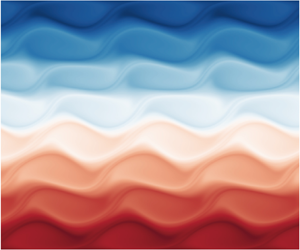
  ${\textit {Ri}}=1$, multiple layers of billow vortices emerge from the initial perturbations and stay in a very organized pattern. These vortices travel horizontally with the background shear velocity and merge with each other. Finally, the flow enters the layering state with convection layers separated by sharp interfaces. This process is illustrated here by figure 2 which depicts the typical density fields for $(Ra, \varLambda, Ri)=(10^6, 2, 2)$ and $(10^7, 2, 2)$. As shown in figure 2(a), multiple layers of vortices appear, and the number of layers is determined by the vertical wavenumber $k_z^i$ of the initial perturbation (2.9a–c). At this moment, we consider the flow to be in the initial stage. As the flow progresses into the second stage, which we refer to as the transitional stage, these vortices grow in size and begin merging both horizontally and across layers, as seen in figure 2(b). Eventually, the vortices disappear and layered structures dominate, as shown in figures 2(c) and 2(d). We refer to this stage as the final stage. The number of layers in the final stage varies for different parameters, but it is unlikely to be determined by a large $k_z^i$. For even higher value of $Ra=10^8$, YVLC22 reports six layers exist. Similarly, Radko (Reference Radko2016) demonstrates that the layer thickness is not controlled by the vertical shear scale, which is in a sinusoidal form. All these findings imply the existence of an intrinsic length scale dictating the layer size, which is independent of the initial perturbations or the background forces.

Figure 2. The instantaneous density fields for the case with  $Ra=10^6, \varLambda =2, Ri=2$ at (a) $t=40$, (b) $t=400$ and (c) $t=4000$. (d) The instantaneous density field for the case with $Ra=10^7, \varLambda =2, Ri=2$ at $t=12\,000$.
The above evolution process can be quantitatively illustrated by figure 3, which plots the time history of the global transport quantities and the dominant horizontal wavenumber for the case with  ${\textit {Ra}}=10^6, \varLambda =2$ and ${\textit {Ri}}=2$. The global quantities include the two Nusselt numbers ${\textit {Nu}}_\theta$ and ${\textit {Nu}}_s$, and the Reynolds number ${\textit {Re}}_z$ defined by the vertical r.m.s. velocity. The dominant horizontal wavenumber $k_x$ is extracted by conducting the fast Fourier transform (FFT) of the instantaneous density field and determining the wavenumber with the maximal mode amplitude. Instead of $k_x$, we plot the rescaled wavenumber
 \begin{equation} K_x=\frac{\varGamma}{2{\rm \pi}}k_x, \end{equation}
which is equal to the number of wave patterns within the width of flow domain.

Figure 3. The time evolution of (a) the vertical Reynolds number, (b) the temperature Nusselt number, (c) the salinity Nusselt number and (d) the horizontal wavenumber (rescaled by  $\varGamma /2{\rm \pi}$) for the case with $Ra=10^6, \varLambda =2, Ri=2$. Panels (a i, b i, c i, d i) show the zoom-in plots of the initial period. The black, yellow and blue lines denote the initial, transitional and final stages, respectively.
Three stages can be identified and displayed by different colours in figure 3. Starting from the initial field, linear instability occurs due to the initially unstable density stratification. During this stage, both Nusselt numbers and Reynolds number increase until they saturate, as the nonlinear effect becomes strong enough. This can be observed in the segment marked by the black lines in figure 3(a–d). The strong nonlinear effect arises from the interactions between large vortices at different heights, hindering their continued growth, as shown in figure 2(b). As will be shown below, the dominant wavenumber  $K_x$ is determined by the linear instability mechanism. As the flow enters the transitional stage, all three global quantities fluctuate around certain values, while the dominant wavenumber $K_x$ remains constant. As the flow reaches the end of this stage and transitions towards the final stage, the Reynolds number ${\textit {Re}}_z$ starts to increase, and fluctuations of the global quantities become stronger. Meanwhile, the horizontal dominant wavenumber $K_x$ gradually decreases, indicating that the vortices grow in size and merge with each other. Note that this merging is different from that in pure Kelvin–Helmholtz instability where the vortices merge in pairs. The transitional stage is marked by the yellow colour in figure 3.
The final stage is characterized by a dominant horizontal wavenumber  $K_x$ equal to unity. For the case shown in figure 3 with ${\textit {Ra}}=10^6$, $\varLambda =2$ and ${\textit {Ri}}=2$, the final state is characterized by two layers separated by one sharp internal interface, as depicted in figure 2(c). For the case with the same $\varLambda$ and ${\textit {Ri}}$ but a higher Rayleigh number ${\textit {Ra}}=10^7$, three layers with two internal interfaces exist in the final state, as seen in figure 2(d). We refer to this type of final state as the layering state, which has at least one internal interface and more than one layer. During the layering state, the global transport quantities exhibit significant fluctuations, especially the salinity Nusselt number. These fluctuations are mainly caused by the spatial oscillation of the internal interfaces.
Two other types of final stages with  $K_x=1$ are also obtained for different parameters. One is the convection type, where the entire bulk consists of only one convection layer. The other is the laminar state in which no flow motions other than the background shear can be sustained. We distinguish between the layering and the convection states because the latter does not have internal interfaces, and the convection layer directly interacts with the boundary layers adjacent to the two plates. Denoting the number of layers at the final state by $N_l$, the layering state has $N_l>1$, the convection state has $N_l=1$ and the laminar state has $N_l=0$. We also mark the time $t_f$ when the dominant wavenumber $K_x$ first decreases to unity and the flow reaches the final state. Both $N_l$ and $t_f$ are listed in table 1.
The relationships between  $N_l$, $t_f$ and ${\textit {Ri}}$ are complex. For $\varLambda =2$, as ${\textit {Ri}}$ increases or the background shear weakens, $N_l$ first decreases to unity and then increases for moderate ${\textit {Ri}}$. When ${\textit {Ri}}$ is large enough, $N_l$ suddenly decreases to zero without any layering state being observed. For $\varLambda =3$, however, the layering state is absent for all the cases considered here; that is, $N_l=1$ for small ${\textit {Ri}}$ and $N_l=0$ for large ${\textit {Ri}}$. These unusual behaviours are due to the fact that the layering state can be sustained by either the shear or the DDC motions, as we will demonstrate in § 3.2. The time $t_f$ varies dramatically for different types of final stages. When the final state is the laminar type, all the initial flow motions decay very quickly, resulting in a small $t_f$ of approximately $10^2$. In contrast, the time needed for the layering state to be established is relatively longer, usually reaching the order of $10^3$. For the convection state, $t_f$ is extremely large compared with the adjacent layering or laminar cases. For example, $t_f=28\,000$ for ${\textit {Ra}}=10^6, {\textit {Ri}}=1, N_l=1$, while $t_f=2100$ for ${\textit {Ra}}=10^6, {\textit {Ri}}=1.5, N_l=2$. In figure 4, we plot the time history of the dominant wavenumber $K_x$ and the spatially averaged density profile for the former case. The system remains in a state with $K_x\approx 3$ for a very long time period, exceeding 20 000 time units. The bulk consists of two strongly oscillating interfaces separating three layers. The distance between the two interfaces gradually increases, and the top and bottom layers diminish within the time period $17\,000< t<30\,000$, after which the bulk reaches the final convection state. This long-term middle stage with $K_x>1$ appears in all cases with $N_l=1$, resulting in large $t_f$. This phenomenon seems to occur when the shear is competitive with the stable density stratification, namely ${\textit {Ri}}_\rho \sim 1$.

Figure 4. The time evolution of (a) the horizontal wavenumber (rescaled by  $\varGamma /2{\rm \pi}$) and (b) the density mean profile for the case with $Ra=10^6, \varLambda =2, Ri=1$. In (a) the yellow, blue, and red lines denote the transitional stage, the layering stage and the special middle stage for this case, respectively. The transient initial stage is not shown in the figure. In (b) the instantaneous salinity fields at $t=10\,000$ and $t=35\,000$ are shown below.
Notice that the time scale used here for non-dimensionalization is  $t_1=H/\sqrt {g\beta _{\theta }\varDelta _\theta H}$, which is much shorter than that of the long-term transitional stage. Another relevant time scale is $t_2=H^2/\kappa _{\theta }$, which characterizes the time for temperature diffusing across the whole domain. The ratio of the two time scales is $t_2/t_1=\sqrt {{\textit {Ra}} {\textit {Pr}}}$. For ${\textit {Ra}}=10^7, {\textit {Pr}}=10$, this yields $t_2=10\,000t_1$, which is of the same order of magnitude as the duration of the transitional stage. This suggests to some extent that the long-term evolution of the flow field during the transitional stage is dominated by temperature diffusion. Similar to YVLC22, we calculate the corresponding dimensional quantities for the ocean environment. We choose $\beta _{\theta }=6.3\times 10^{-5}\ {\rm K}^{-1}$, $\kappa _{\theta }=1.4\times 10^{-7}\ {\rm m}^2$ s $^{-1}$, $g=9.8\ {\rm m}\ {\rm s}^{-2}$ and $\varDelta _\theta =0.05$ K, which is the typical value of the temperature difference across an interface in the Arctic Ocean (Shibley et al. Reference Shibley, Timmermans, Carpenter and Toole2017). Then, for ${\textit {Ra}}=10^6$, $H\approx 0.2$ m and $t_2\approx 3$ days; for ${\textit {Ra}}=10^7$, $H\approx 0.4$ m and $t_2\approx 13$ days, respectively. The longest simulation time in our present work is approximately 47 days ( $Ra=10^6, \varLambda =3, Ri=0.7$). Considering that the variability of large-scale oceanic currents is generally seasonal (Rudels Reference Rudels2015), steady shear on the time scale of $t_2$ should be relatively easy to maintain.
It is necessary to point out that a stronger initial perturbation, i.e. larger  $\delta$, is unlikely to change the final state. Further theoretical analyses, given in § 4, reveal that larger $\delta$ only results in larger wavenumber of the initial linear unstable mode, which requires stronger shear to be sustained. This explains why, in test cases where the final state is laminar, increasing $\delta$ merely accelerates the return of the flow field to its laminar state. For cases reaching the convection or layering state, even when there is sufficiently strong shear to sustain the initial modes with larger wavenumbers induced by larger $\delta$, the vortices will gradually merge during the transitional stage and ultimately follow the same path to the same final state. Therefore, the initial perturbation only affects the wavenumbers of the unstable modes in the initial stage, determining whether the flow can be sustained. Once the flow enters the transitional stage, the subsequent evolution process will no longer be influenced by the initial perturbation.
3.2. The statistical properties of the final stage
We now examine the statistic behaviours of the final stage for the cases that reach the layering or convective state. The time period  $t_s$ during which the statistics are sampled is set to be equal to or greater than $1000$, as shown in table 1. As a confirmation of the statistically steady state, all the statistics are calculated over the first and the second halves of the sampling period, and the two values agree with each other.
Figure 5 presents the mean scalar profiles  $\overline {\langle s\rangle }_h$ and $\overline {\langle \theta \rangle }_h$ for all cases. Hereafter, the overbar denotes the time-averaged value of the respective variable. The staircase shape is evident in the cases with a layering final state. The interface regions in these mean profiles are thicker than those in the instantaneous fields shown in figure 2. This is caused by the strong spatial oscillation of the sharp interfaces which smooths the averaged profiles. Notably, the typical heights of convection layers for both ${\textit {Ra}}=10^6$ and ${\textit {Ra}}=10^7$ are much larger than the vertical wavelength of the initial perturbation (2.9a–c). Therefore, the final staircase configuration results from the nonlinear interactions among the travelling vortices during the second stage and the emerging layers during the transition from the second to the final stage.

Figure 5. The temporal and horizontal averaged scalar profiles in the final stage for the case with (a)  $Ra=10^6, \varLambda =2$, (b) $Ra=10^6, \varLambda =3$ and (c) $Ra=10^7, \varLambda =2$. The blue solid lines denote the salinity profiles and the yellow dashed lines denote the temperature profiles.
The profiles exhibit very complex and non-monotonic variations as  ${\textit {Ri}}$ changes, especially for the two groups with $\varLambda =2$. For the group with ${\textit {Ra}}=10^6$ and $\varLambda =3$ (see figure 5b), the bulk becomes laminar for ${\textit {Ri}}=0.8$. When ${\textit {Ri}}\leq 0.7$, the bulk becomes nearly homogeneous for both mean temperature and salinity, and the homogeneous layer is bounded by two layers with linear mean profiles from the top and bottom. As ${\textit {Ri}}$ decreases, the homogeneous layer shrinks in the vertical direction. In the other two groups with $\varLambda =2$ (see figure 5a,c), the laminar state exists when ${\textit {Ri}}$ is large enough. As ${\textit {Ri}}$ becomes smaller, the number of layers in the bulk varies non-monotonically. Taking the group with ${\textit {Ra}}=10^7$ and $\varLambda =2$ for example, three layers appear for $3\geq {\textit {Ri}}\geq 1$. When ${\textit {Ri}}$ decreases from $1$ to $0.5$, the three-layer state is replaced by a one-layer configuration. As ${\textit {Ri}}$ further decreases to $0.3$, it seems that another internal interface appears near the top plate. However, a significant difference between this case and the layering state at intermediate Richardson numbers is that, in the former, the mean profiles exhibit different structures for the two components, while in the latter, both mean temperature and salinity profiles have the same number of layers. Therefore, this case does not have well-defined layering morphology. Another similar case is the one with ${\textit {Ra}}=10^6$, $\varLambda =2$ and ${\textit {Ri}}=0.3$, namely the case shown by the most left-hand profiles in figure 5(a). As will be shown next, these two cases exhibit very different behaviours in fluxes compared with the well-defined layering state at the intermediate Richardson numbers.
To illustrate these different regimes in more detail, we will examine the fluxes and the thicknesses of the interfaces for the statistically steady state. The dimensionless convective and conductive fluxes for the salinity and temperature are defined as
 \begin{equation} F_s^v=\frac{ w^* s^* }{\kappa_s \varDelta_s H^{-1}}, \quad F_s^d=\frac{-\partial_z s^* }{\varDelta_s H^{-1}}, \quad F_\theta^v= \frac{ w^* \theta^* }{\kappa_\theta \varDelta_\theta H^{-1}}, \quad F_\theta^d= \frac{ - \partial_z \theta^* }{ \varDelta_\theta H^{-1}},\end{equation}
in which the superscripts  $v$ and $d$ denote the convective and conductive fluxes, respectively. Figure 6 shows the mean vertical profiles of the quantities in (3.2a–d) for two typical cases. One case has only one convection layer and no internal interface with ${\textit {Ra}}=10^6, \varLambda =3, {\textit {Ri}}=0.3$, while the other case has three convection layers and two internal interfaces with ${\textit {Ra}}=10^7, \varLambda =2, {\textit {Ri}}=3$. Notice that for the statistically steady state, the sum of the convective and conductive fluxes should be constant at any height. Within the boundary interfaces, the convective fluxes tend to zero, and the vertical transport is dominated by molecular diffusion. Figures 6(a) and 6(b) clearly show two thicker boundary interfaces. Within the internal interfaces, however, the convective fluxes are smaller than those in the convection layers but are not negligible, as shown in figures 6(c) and 6(d). This is because the internal interfaces experience very strong spatial oscillation, causing the convective fluxes to increase accordingly. As a result, the vertical extent of the internal interfaces appears blurred, making it challenging to define their precise thicknesses.

Figure 6. The convective and conductive profiles for the two scalar components for the cases with (a,b)  ${\textit {Ra}}=10^6, \varLambda =3, {\textit {Ri}}=0.3$ and (c,d) ${\textit {Ra}}=10^7, \varLambda =2, {\textit {Ri}}=3$.
To investigate the diffusive interfaces systematically, we choose to analyse the boundary interfaces, of which the thickness can be defined as the distance between the location of the first peak of the standard deviation profile and the corresponding boundary, as shown in figure 7. Hereafter, the thicknesses of the temperature and salinity boundary interfaces are denoted by  $h_\theta$ and $h_s$, respectively. Figure 8 displays the instantaneous scalar fields for the same two cases depicted in figures 6 and 7. For the case with ${\textit {Ra}}=10^6, \varLambda =3, {\textit {Ri}}=0.3$, the boundary interfaces are rather thick, with their thicknesses comparable to that of the central convection layer. In contrast, for the case with ${\textit {Ra}}=10^7, \varLambda =2, {\textit {Ri}}=3$, the boundary interface thicknesses are much smaller than those of the convection layers. Furthermore, as mentioned earlier, due to intense oscillations, the internal interfaces occupy a relatively larger vertical range, as shown in figure 7(b).

Figure 7. The standard deviation profiles for the two scalar components for the cases with (a)  ${\textit {Ra}}=10^6, \varLambda =3, {\textit {Ri}}=0.3$ and (b) ${\textit {Ra}}=10^7, \varLambda =2, {\textit {Ri}}=3$. Panel (c) presents a zoom-in plot of the profiles shown in (b). In both (a) and (c) the corresponding thicknesses are marked by the vertical solid lines.

Figure 8. The instantaneous flow fields for the cases with  ${\textit {Ra}}=10^6, \varLambda =3, {\textit {Ri}}=0.3$ (a,c,e) and ${\textit {Ra}}=10^7, \varLambda =2, {\textit {Ri}}=3$ (b,d,f). Panels (a,b), (c,d) and (e,f) represent temperature, salinity and density, respectively.
Figure 9 plots the variations of the ratio  $h_\theta /h_s$, the time-averaged flux ratio $\bar {\gamma }$ and the time averaged Nusselt numbers. The figure includes only cases that do not transition into the laminar state. All four quantities exhibit much larger values at high ${\textit {Ri}}$ compared with those at low ${\textit {Ri}}$. In the theoretical model proposed by Linden & Shirtcliffe (Reference Linden and Shirtcliffe1978) for the diffusive DDC flow, the transport within the interfaces is dominated by the diffusion process. Then, since temperature diffuses much faster than salinity, the thickness of the thermal diffusion core is much larger than that of the salinity diffusion core, and the ratio of the two thicknesses should be approximately equal to $1/\sqrt {\tau }=10$. The flux ratio, meanwhile, should be equal to $\sqrt {\tau }=0.1$. Figures 9(a) and 9(b) indicate that, for large ${\textit {Ri}}$, $h_\theta /h_s$ is approximately $8$ and $\bar {\gamma }$ exceeds $0.08$, respectively. These two values closely match the theoretical predictions provided by the model of Linden & Shirtcliffe (Reference Linden and Shirtcliffe1978). This strongly suggests that under conditions of high ${\textit {Ri}}$ or weak shear, the flow and the transport are dominated by the diffusive DDC process. The model of Linden & Shirtcliffe (Reference Linden and Shirtcliffe1978) also suggests that near the interfaces, the unstable temperature layer could release plumes which transport both heat and salt. Such a scenario is clearly observable in figure 8(b,d,f).

Figure 9. The Richardson number versus the time-averaged (a) ratio of temperature and salinity boundary layer thicknesses, (b) total flux ratio, (c) salinity Nusselt number and (d) temperature Nusselt number for the cases with different  $Ra$ and $\varLambda$. The solid symbols denote the DDC-dominated regime, while the open symbols denote the shear-influenced regime.
For small  ${\textit {Ri}}$, as shown in figure 8(a,c,e), the plumes are severely tilted due to the strong shear. As a result, weaker transport and smaller Nusselt numbers are observed. The thickness ratio $h_\theta /h_s$ approaches unity as ${\textit {Ri}}$ decreases. The decrease in ${\textit {Nu}}_\theta$ as ${\textit {Ri}}$ decreases is smaller than the decrease in ${\textit {Nu}}_s$, and as a result, the flux ratio $\bar {\gamma }$ also decreases with ${\textit {Ri}}$. This regime at small ${\textit {Ri}}$ is referred to as the shear-influenced regime, as opposite to the DDC-dominated regime at large ${\textit {Ri}}$. Figure 10 displays all the cases in different regimes, with the vertical dashed line marking the boundary between the shear-influenced regime and the DDC-dominated regime. Another boundary between the DDC-dominated regime and the laminar regime will be theoretically predicted in § 4. Comparing figures 10 and 5, it is evident that the well-defined staircases only occur in the DDC-dominated regime with weak background shear. As a final demonstration of the difference between the DDC-dominated and shear-influenced regimes, we calculate the local density ratio in the diffusive core of the interface as
 \begin{equation} \varLambda_{in}=\frac{\beta_s S_z^*} {\beta_\theta \varTheta_z^*} =\frac{\varLambda Nu_s}{ Nu_\theta}=\frac{\gamma}{\tau},\end{equation}
in which  $S_z^*$ and $\varTheta _z^*$ are the dimensional mean vertical gradients of salinity and temperature, respectively. The values of $\varLambda _{in}$ are summarized in table 1. According to the model of Linden & Shirtcliffe (Reference Linden and Shirtcliffe1978), one has $\varLambda _{in}\approx \tau ^{-1/2}=10$ for the diffusive DDC interfaces. Indeed, for the cases in the DDC-dominated regime, $\varLambda _{in}$ is large and close to 10. In contrast, in the shear-influenced regime, this quantity is much smaller.

Figure 10. The regime diagram displaying the shear-influenced regime (open symbols), the DDC-dominated regime (blue and yellow solid symbols) and the laminar regime (grey symbols).
4. Theoretical model for the development of layering
4.1. Linear development of the initial stage
In the previous section, we identified three different stages of the flow evolution and discussed the statistics and transport of the final stage. We now present theoretical analyses on how the flow is triggered and develops from the initial conditions (2.9a–c). In this section, we focus on the initial stage and conduct the linear stability analysis for the governing equations (2.3a)–(2.3c) with the initial conditions (2.9a–c). The second transitional stage will be discussed in the next section.
Specifically, we expand the variables in ascending powers of a small dimensionless parameter  $\epsilon$, i.e.
 \begin{equation} \{\psi, \theta, s\}^T= \{\psi_0, \theta_0, s_0\}^T+ \epsilon\{\psi_1, \theta_1, s_1\}^T+ O(\epsilon^2), \end{equation}
in which  $\{\psi _0, \theta _0, s_0\}^T$ is the base state and $\{\psi _1, \theta _1, s_1\}^T$ is the linear solution. To satisfy the initial conditions (2.9a–c), we set the base state as
 \begin{equation} \psi_0=0, \quad \theta_0=1-z-\delta \sin(k^i_z z)\, {\rm e}^{-\omega_\theta t}, \quad s_0=1-z-\delta \sin( k^i_z z)\, {\rm e}^{-\omega_s t}, \end{equation}
in which  $\omega _\theta ={k^i_z}^2/\sqrt {{\textit {Ra}}{\textit {Pr}}}$ and $\omega _s={k^i_z}^2/({\textit {Le}}\sqrt {{\textit {Ra}}{\textit {Pr}}})$. Substituting the parameters with their numerical values used in the DNS, we obtain $(\omega _\theta, \omega _s)=(0.45,0.0045)$ for $Ra=10^6$ and $(\omega _\theta, \omega _s)=(0.25,0.0025)$ for $Ra=10^7$. It is easy to find out that the state (4.2a–c) is a trivial solution of the (2.3a)–(2.3c). Substituting (4.1) and (4.2a–c) into the governing equations (2.3a)–(2.3c), we obtain the linearized equations at the order $\epsilon$ as follows:
 $$\begin{gather} \partial_t \nabla^2 \psi_1 =- \frac{z-1/2}{\sqrt{Ri}}\partial_x \nabla^2 \psi_1+ \frac{\sqrt{Pr}}{\sqrt{Ra}}\nabla^4\psi_1-( \partial_x \theta_1-\varLambda\partial_x s_1) , \end{gather}$$
 $$\begin{gather}\partial_t \theta_1 =-(1+k^i_z \delta \cos( k^i_z z)\, {\rm e}^{-\omega_\theta t})\partial_x \psi_1 -\frac{z-1/2}{\sqrt{Ri}} \partial_x \theta_1+\frac{1}{\sqrt{Ra Pr}}\nabla^2\theta_1, \end{gather}$$
 $$\begin{gather}\partial_t s_1 =-(1+ k^i_z \delta \cos( k^i_z z)\, {\rm e}^{-\omega_s t})\partial_x \psi_1 -\frac{z-1/2}{\sqrt{Ri}} \partial_x s_1+\frac{\sqrt{Pr}}{\sqrt{Ra}Sc}\nabla^2s_1. \end{gather}$$
Equations (4.3a)–(4.3c) form an eigenvalue problem when assuming the normal-mode solution as
 \begin{equation} \{\psi_1, \theta_1, s_1\}^T = {\rm e}^{\omega_it}\{\hat{\psi}_1(z), \hat{\theta}_1(z), \hat{s}_1(z)\}^T\, {\rm e}^{j(k_x x-\omega_rt)}+{\rm c.c.}\end{equation}
Here,  $\{\hat {\psi }_1(z), \hat {\theta }_1(z), \hat {s}_1(z)\}^T$ are the vertical shape functions, $\omega _i$ and $\omega _r$ are the real and imaginary temporal growth factors, respectively, $k_x$ is the horizontal wave number, $j$ is the imaginary unit and c.c. stands for the conjugate complex. The boundary conditions then
 $$\begin{gather} \hat{\psi}_{1}=0, \quad \partial_z^2 \hat{\psi}_{1}=0,\quad \hat{\theta}_{1}=0, \quad \hat{s}_{1}=0,\quad {\rm at} \quad z=0, \end{gather}$$
 $$\begin{gather}\hat{\psi}_{1}=0, \quad \partial_z^2 \hat{\psi}_{1}=0,\quad \hat{\theta}_{1}=0, \quad \hat{s}_{1}=0,\quad {\rm at} \quad z=1. \end{gather}$$
 The first term on the right-hand sides of both (4.3b) and (4.3c) explicitly contain time  $t$, and this term represents the exponential decay of the initial sinusoidal perturbation. Since we are interested in the initial development of the normal modes at small $t$, we set $\exp (-\omega _\theta t) \approx 1$ and $\exp (-\omega _s t) \approx 1$ in (4.3b) and (4.3c). That is, we first investigate the linear instability under the assumption that the initial perturbation remains unchanged. Afterwards, the influence of the time decay terms in the perturbations will be examined. The Prandtl number and the Schmidt number are set as 10 and 1000, respectively. Then the eigenvalue problem is influenced by the control parameters ${\textit {Ra}}$, $\varLambda$ and ${\textit {Ri}}$, as well as the parameters for the initial perturbation $\delta$ and $k^i_z$. For a given combination of $(\delta, k^i_z, {\textit {Ra}}, \varLambda )$, the eigenvalue problem is solved numerically for a wide range of $k_x$ and ${\textit {Ri}}$. The Chebyshev polynomial expansion is used in the $z$-direction with $300$ grid points. Computations are also conducted with $600$ grid points and the results are similar between the two resolutions. The growth rates $\omega _i$ and $\omega _r$, along with the shape functions, are solved for each $k_x$.
Figure 11 displays the results of linear instability analyses for three different combinations of  $(\delta, k^i_z, {\textit {Ra}}, \varLambda )$ over the range $0.1\le {\textit {Ri}}\le 10$. Here, $\delta$ and $k^i_z$ are chosen to be the same as those used in DNS, and $({\textit {Ra}}, \varLambda )=(10^6, 2)$, $(10^6, 3)$ and $(10^7, 2)$, respectively. For all three combinations of $({\textit {Ra}}, \varLambda )$, unstable wavenumbers exist over the entire range of $0.1\le {\textit {Ri}}\le 10$. The wavenumber of the fastest-growing mode is indicated by the dashed curves. The initial dominant wavenumber $k_x^w$ is also extracted from the flow fields at the beginning of DNS, and marked by the circle symbols. The predictions of the linear instability theory agree with DNS results. Closed circles indicate the cases that develop into layering, while open circles mark the cases which become laminar at the end. Thus, although the finite-amplitude perturbations at the beginning can trigger linearly unstable modes, these modes do not necessarily result in layering. For comparison, Radko (Reference Radko2016) and Radko (Reference Radko2019) demonstrate that steady sinusoidal shear and time-varying uniform shear can excite linear instability without initial perturbations, respectively. For a single uniform shear, which has no inflection points in its vertical profile, it is both inherently stable and incapable of inducing diffusive DDC instability. Existing studies indicate that a sinusoidal or stochastic external force, varying in time or space, must be needed for triggering unstable modes in the linearly stable diffusive DDC regime.

Figure 11. The contour of  $\omega _i$ as a function of $k_x$ and ${\textit {Ri}}$ for the cases with (a) $({\textit {Ra}},\varLambda )=(10^6, 2)$, (b) $(10^6, 3)$ and (c) $(10^7, 2)$, respectively. The solid lines denote the neutral curves with $\omega _i=0$ and the dashed lines denote the fastest-growing modes. Here $k_x^w$ extracted from DNS results is displayed by circles, with closed symbols for the cases developing into layering or convection state and the open ones for those becoming laminar.
The above results about the linearly unstable modes are derived for very small  $t$ at the beginning of the flow evolution, since both $\exp (-\omega _\theta t)$ and $\exp (-\omega _s t)$ in (4.3) are set to unity. As time increases, the base flow changes due to the decay of initially finite-amplitude perturbation. Additionally, the growth rate of the unstable modes is expected to vary with time. However, further investigation indicates that the flow evolution is dominated by similar linear instability for a relatively long time, even as the initial perturbation decays. To demonstrate this, we conduct linear stability analysis at different times for the case with $(\delta, k^i_z, {\textit {Ra}}, \varLambda, {\textit {Ri}})=(0.05, 12{\rm \pi}, 10^6, 2,2)$. Specifically, for a given time $t$, the corresponding values of $\exp (-\omega _\theta t)$ and $\exp (-\omega _s t)$ are set in (4.3) and the eigenvalue problem is solved accordingly. In other words, we will use the initial conditions (4.2a–c), which decay with time $t$, as the new initial conditions, and assume they do not change with time. Figure 12(a) displays the growth rates of different wavenumbers at different time. The system is linearly unstable up to $t\approx 100$. The most unstable wavenumber, as marked by the dashed line, and the corresponding growth rate both change slightly with time. This indicates that for a considerable initial time period, the linearly unstable modes are similar. Therefore, assuming the initial perturbations remain unchanged for linear stability analysis is reasonable, explaining why we obtain consistent results between linear theory and DNS under this assumption. The underlying reason for this phenomenon is that the time decay coefficients $\omega _\theta$ and $\omega _s$ are very small for large $Ra$, particularly $\omega _s$, which is much smaller than the typical growth rate of the unstable modes. Thus, during the time period when the unstable modes are sufficiently developed, it can be assumed that the initial perturbations remain unchanged.

Figure 12. The temporal growth rate  $\omega _i$ as a function of (a) $(k_x,t)$ at $\delta =0.05$ and (b) $(k_x, \delta )$ at $t=0$ for the case with $(k_z^i, Ra, \varLambda,Ri)=(12{\rm \pi}, 10^6, 2,2)$. The solid line denotes $\omega _i=0$, the dashed line denotes the fastest-growing mode and the dash–dotted line denotes $\delta =1/ k_z^i$.
The influences of the amplitude  $\delta$ on the linear instability are also investigated for the same case at $t=0$, and the results are shown in figure 12(b). Linear instability does occur when $\delta$ is large enough. Interestingly, the critical value of $\delta$ is slightly smaller than $1/k^i_z$. Therefore, the system can be linearly unstable even when the initial perturbation is not strong enough to cause locally unstable stratification.
Based on the results shown in figure 12, we can calculate the temporal growth of the most unstable mode at  $t=0$ with wavenumber $k^w_x$, and compare it with the DNS results. The comparison is shown in figure 13 for three cases with different parameters. For the DNS results, the dominant horizontal mode of the density anomaly
 \begin{equation} \rho'=\rho-\langle\rho\rangle_h=\varLambda(s-\langle s \rangle_h)-(\theta-\langle \theta \rangle_h) \end{equation}
is extracted using the FFT, and the temporal variation of the amplitude  $\delta _p$ is shown by the solid lines. Then, starting with $\delta _p$ at $t=1$, the growth of the amplitude is also calculated by using the growth rate $\omega _i(t)$ given by the linear theory. Notice that the growth rate $\omega _i(t)$ varies with time. The amplitude is then computed by the integration
 \begin{equation} \delta_p(t) = \delta_p|_{t=1} \times \exp\left[\int_{\tau=1}^t\omega_i(\tau) \, {\rm d}\tau\right], \end{equation}
and the results are shown by the dashed lines in figure 13. Remarkably, the linear theory can predict the growth of amplitude up to  $t\approx 30$. This strongly implies that, although the base flow constantly changes as the initial perturbation decays, the growth of the fluctuation motions is dominated by the linear instability mechanism.

Figure 13. The amplitude of density anomaly versus time for the cases with (a)  $({\textit {Ra}},\varLambda,{\textit {Ri}})=(10^6, 2,2)$, (b) $(10^6, 3,0.5)$ and (c) $(10^7, 2,1)$, respectively. The blue solid lines denote the DNS results, and the red dashed lines denote the values calculated by linear growth rates.
For the completeness of the linear stability analysis, we plot the flow field corresponding to the most unstable mode during the linear instability stage, as shown in figure 14. The parameters used are  $(\delta, k^i_z, {\textit {Ra}}, \varLambda, {\textit {Ri}})=(0.05, 12{\rm \pi}, 10^6, 2, 2)$. Both the leftward travelling mode with $\omega _r<0$ and the rightward travelling one with $\omega _r>0$ are shown. The perturbations mainly occur at the centre part of the domain, and the flow patterns are very similar to the flow field given by DNS, e.g. see figure 2(a). Notice that the pattern of two counter-propagating waveforms occurs at the initial stage for all cases, which may be due to the set-up of the background shear flow, i.e. the streamwise velocity is positive in the upper region and negative in the lower region.

Figure 14. (a) The imaginary part and the real part of the shape functions for temperature and salinity and (b) the corresponding density field of the linear fastest-growing mode at  $t=0$ for the case with $(\delta, k^i_z, {\textit {Ra}}, \varLambda, {\textit {Ri}})=(0.05, 12{\rm \pi}, 10^6, 2, 2)$. The leftward travelling mode with $\omega _r<0$ and the rightward travelling one with $\omega _r>0$ are denoted by the yellow dashed lines and blue solid lines, respectively, in (a) and by the arrows in (b).
4.2. Sustenance of the transitional stage
For all the cases simulated in the current study, linear instability occurs as discussed in the previous section. However, not all of them develop into layering or convective states. When  ${\textit {Ri}}$ is large, the fluctuation motions induced by the initial linear process die out, and the flow returns to the laminar state. Only when ${\textit {Ri}}$ is smaller than a certain critical value ${\textit {Ri}}^c$ for a given ${\textit {Ra}}$ and $\varLambda$, do the fluctuation motions sustain and lead to layering or convection states. Here we will employ the energy method and theoretically determine the critical value ${\textit {Ri}}^c$ and compare the theoretical predictions with DNS results.
We start with the kinetic energy equation, which can be obtained by conducting the inner product between the momentum equations (2.1a) and (2.1b) and the velocity  $\boldsymbol {u}^*$. With the help of the incompressible equation (2.1e), the non-dimensional equation for the kinetic energy $e=|\boldsymbol {u}|^2/2$ reads
 \begin{align} & \frac{\partial e }{\partial t} + \boldsymbol{\nabla}\boldsymbol{\cdot} (\boldsymbol{u} e) + \frac{z-1/2}{2\sqrt{Ri}}\frac{\partial e}{\partial x}+\frac{1}{\sqrt{Ri}}uw \nonumber\\ &\quad =- \boldsymbol{\nabla}\boldsymbol{\cdot} (\,p\boldsymbol{u}) +\frac{\sqrt{{\textit{Pr}}}}{\sqrt{Ra}} ({\nabla}^2 e - (\boldsymbol{\nabla} \boldsymbol{u})^2) + ( \theta- \varLambda s)w. \end{align}
The above equation can be integrated over the whole domain, and by using the boundary condition (2.6), one can obtain the total kinetic energy balance equation as
 \begin{equation} \frac{\partial E_k}{\partial t}=\varPi_s+\varPi_p-\varPi_d, \end{equation}
in which
 $$\begin{gather} E_k=\frac{1}{2}\langle u^2+w^2 \rangle_V , \end{gather}$$
 $$\begin{gather}\varPi_s=-\frac{1}{\sqrt{Ri}}\langle uw \rangle_V , \end{gather}$$
 $$\begin{gather}\varPi_p=\langle w\theta \rangle_V-\varLambda\langle ws \rangle_V, \end{gather}$$
 $$\begin{gather}\varPi_d=\frac{\sqrt{Pr}}{\sqrt{Ra}}\langle (\partial_x u)^2+(\partial_z u)^2+(\partial_x w)^2+(\partial_z w)^2\rangle_V. \end{gather}$$
Hereafter the bracket  $\langle \cdot \rangle _V$ denotes the volume-averaged quantity. As per the definition, $E_k$ represents the kinetic energy, $\varPi _s$ represents the energy exchange with the background shear, $\varPi _p$ represents the energy exchange with the potential energy and $\varPi _d$ represents the energy dissipation due to viscosity. As an illustration, figure 15 plots these different terms against time for a case with $({\textit {Ra}}, \varLambda, {\textit {Ri}})=(10^6,2,2)$. For this case, the transitional stage lasts until $t=2500$, as marked by the vertical dotted line, and then the system enters the final state. During the transitional stage, both $\varPi _p$ and $\varPi _s$ are positive, indicating that the flow receives kinetic energy from the background shear and the potential energy stored in scalar fields. At this moment, the vertical momentum flux is down-gradient across the wavelike structures. However, neither the background shear nor the potential energy released by scalar field alone can sustain the flow. Only the combination of the two production mechanisms of kinetic energy can overcome the viscous dissipation. During the final layering state, the kinetic energy production due to the release of potential energy is much larger than that due to interactions with the background shear. Additionally, $\varPi _s$ exhibits a strong oscillation and can sometimes become negative. Here, $\varPi _s<0$ means that part of the potential energy is converted into the vertical kinetic energy, and the vertical momentum flux becomes up-gradient, a phenomenon often observed in stably stratified sheared turbulence for high gradient Richardson numbers (Holt, Koseff & Ferziger Reference Holt, Koseff and Ferziger1992; Piccirillo & van Atta Reference Piccirillo and van Atta1997). The oscillation of $\varPi _s$ near zero indicates that the vertical momentum flux frequently changes its direction, which is probably due to the oscillation of the interfaces.

Figure 15. The time evolution of  $\varPi _d, \varPi _p$, $\varPi _s$ and $\varPi _s+\varPi _p$ for the case with $Ra=10^6, \varLambda =2$ and $Ri=2$. The vertical dotted line denotes the boundary between the transitional stage and the final stage.
The above discussions imply that during the transitional stage, the background shear plays an indispensable role. A naïve criterion for the flow to sustain during the transitional stage is
 \begin{equation} \partial E_k / \partial t >0, \quad \mbox{or} \quad \varPi_s+\varPi_p > \varPi_d. \end{equation}
In order to utilize the above criterion, the explicit forms of all terms must be provided, which is practically impossible for the entire flow. Instead, we focus on the dominant mode of the flow during the transitional stage and seek the explicit formulae of  $\varPi _s$, $\varPi _p$ and $\varPi _d$ for the dominant mode. Figure 16 depicts the flow fields of different variables at $t=200$ for the same case shown in figure 15, in which $\theta '=\theta -1+z$ and $s'=s-1+z$ are the temperature and salinity anomalies, respectively. One notices that for different quantities, the dominant wavenumbers in the streamwise direction are similar, while those in the vertical direction are not. Especially, due to the slow diffusion, the salinity anomaly field in figure 16(d) retains most details of the initial finite amplitude perturbation. One of the major characteristics is that positive and negative salinity anomalies stack over each other in the vertical direction, a phenomenon not observed for the other three quantities.

Figure 16. The instantaneous fields of (a) vertical velocity, (b) horizontal velocity, (c) temperature anomaly and (d) salinity anomaly at  $t=200$ for the case with $Ra=10^6, \varLambda =2, Ri=2$.
To develop the explicit formulae for the terms in the energy balance criterion, we discuss the wavenumbers for different flow quantities in detail. As shown in figure 14, the linear fastest-growing mode simultaneously contains a waveform moving forward in the upper region along the flow direction and a waveform moving backward in the lower region. The vertical wavenumbers of these two waveforms are approximately  $4{\rm \pi}$. However, after nonlinear interactions, the upper and lower modes of the transitional stage merge into a single mode, which propagates slowly along one direction. For a relatively long period at the beginning of the transitional stage, the streamwise wavenumber $k_x^w$ of this mode remains the fastest-growing wavenumber predicted by the linear analysis, while the vertical wavenumber $k_z^w$ is approximately $2{\rm \pi}$. This structure can be clearly observed in the vertical velocity field shown in figure 16(a). Furthermore, the flow field in this stage is also influenced by the initial sinusoidal perturbations (2.9a–c). The salinity anomaly field clearly exhibits a vertical wavenumber $k^i_z$, as shown in figure 16(d). The relevant vertical wavenumbers contain both $k_z^w$ and $k^i_z$, which we refer to as the waving mode and the initial mode, respectively. However, their relative strengths differ for different flow quantities. Since the initial salinity perturbation diffuses slowly, the salinity field is most strongly affected by the initial mode during the transitional stage. On the other hand, the initial temperature perturbation diffuses quickly, resulting in a relatively smaller influence on the temperature field. The velocity field, in the absence of initial perturbations, is hardly affected by the initial mode.
Based on the aforementioned analysis, the flow evolution at the beginning of the transitional stage can be assumed to be a quasi-steady process. Therefore, we can now propose the following waving model:
 $$\begin{gather} u = \partial_z \psi=-\delta_\psi^w k_z^w \sin(k_x^w x+k_z^w z)-\delta_\psi^ik_z^i\sin(k^i_zz), \end{gather}$$
 $$\begin{gather}w =-\partial_x \psi= \delta_\psi^w k_x^w \sin(k_x^w x+k_z^w z), \end{gather}$$
 $$\begin{gather}\theta = 1-z +\delta_\theta^w \sin(k_x^w x+k_z^w z)+\delta_\theta^i \sin(k_z^i z), \end{gather}$$
 $$\begin{gather}s = 1-z+\delta_s^w \sin(k_x^w x+k_z^w z) +\delta_s^i\sin(k_z^i z), \end{gather}$$
in which
 $$\begin{gather} \psi = \delta_\psi^w\cos(k_x^w x+k_z^wz )+\delta_\psi^i\cos(k_z^iz), \end{gather}$$
 $$\begin{gather}\delta_\psi^w =-\delta_u^w/k_z^w=\delta_w^w/k_x^w, \end{gather}$$
 $$\begin{gather}\delta_\psi^i =-\delta_u^i/k_z^i. \end{gather}$$
Hereafter, the superscripts  $w$ and $i$ denote the waving mode and the initial mode, respectively. Here $\delta _u^w, \delta _w^w, \delta _\theta ^w$ and $\delta _s^w$ are the amplitudes of the waving mode for horizontal velocity, vertical velocity, temperature and salinity, respectively, while $\delta _u^i, \delta _\theta ^i$ and $\delta _s^i$ are the respective amplitudes of the initial mode. Their values are determined by the interplay between the linear fastest-growing mode and the initial perturbations. As stated before, the velocity field is hardly affected by the latter, thus $\delta _u^i$ should be small, and $\delta _u^w$ and $\delta _w^w$ are close to the amplitudes of the linear mode when the flow enters the transitional stage. For the salinity field, on the other hand, the corresponding linear mode is largely inhibited by the initial salinity perturbation, which diffuses slowly, thus $\delta _s^w$ is small and $\delta _s^i$ is close to $\delta$, namely the amplitude of the initial perturbations. The initial temperature perturbation diffuses quickly, resulting in a small $\delta _\theta ^i$. However, it still influences the linear mode to some extent, resulting in a relatively small $\delta _\theta ^w$ compared with $\delta _u^w$ and $\delta _w^w$. Based on the above analysis, we can conclude $\delta _s^w \ll \delta _\theta ^w < \delta _u^w$, which will be used later.
It is noteworthy that the model (4.12) does not satisfy the vertical boundary conditions; hence, it serves as an approximate model for describing the bulk region. Substituting (4.12) into (4.10), we can obtain
 $$\begin{gather} E_k^w ==\frac{1}{4}{\delta_\psi^w}^2 ({k_x^w}^2+{k_z^w}^2), \end{gather}$$
 $$\begin{gather}\varPi_s^w ==\frac{1}{2\sqrt{Ri}}{\delta_\psi^w}^2 k_x^w k_z^w, \end{gather}$$
 $$\begin{gather}\varPi_p^w = \frac{1}{2}(\delta_\theta^w-\varLambda\delta_s^w) \delta_\psi^w k_x^w , \end{gather}$$
 $$\begin{gather}\varPi_d^w = \frac{\sqrt{Pr}}{2\sqrt{Ra}}{\delta_\psi^w}^2({k_x^w}^2+{k_z^w}^2)^2. \end{gather}$$
It can be observed that the initial mode contributes negligibly to the volume-averaged energy. Since  $\delta _s^w \ll \delta _\theta ^w$, $\varPi _p^w$ mainly comes from the energy released from the temperature field.
By substituting (4.14) into the criterion (4.11), we arrive at the following condition for the transitional stage which can sustain
 \begin{equation} \frac{1}{\sqrt{Ri}} \geq \frac{\sqrt{Pr}}{\sqrt{Ra}}\dfrac{((k_x^w)^2+(k_z^w)^2)^2}{k_x^w k_z^w}-c^w, \end{equation}
in which
 \begin{equation} c^w=\frac{\delta_\theta^w-\varLambda\delta^w_s}{{\delta^w_\psi}k^w_z} \approx\frac{\delta_\theta^w}{\delta^w_{u}}, \end{equation}
is an empirical coefficient. Since  $\delta _\theta ^w< \delta _u^w$, $c^w$ should be smaller than unity. In this paper we adopt $c^w=0.8$ based on the numerical results. The specific value of $c^w$ may be influenced by both the initial linear instability and the subsequent nonlinear evolution, which needs detailed investigation in future work. The term on the left-hand side of (4.15) represents the dimensionless vertical shear rate, while the two right-hand terms represent the dimensionless rates of viscous dissipation and potential energy release, respectively. Therefore, the physical interpretation here is that the background shear needs to provide enough energy to compensate for the difference between the consumption of viscous dissipation and the supply of potential energy, thus sustaining the flow. For $Ri\sim O(1)$ in the current work, when condition (4.15) is satisfied, the magnitudes of the two right-hand terms are comparable. As discussed before, $k_z^w$ can be set to $2{\rm \pi}$. Then, for given ${\textit {Ra}}$ and $\varLambda$, one can readily calculate the value of $k_x^w$ at which the equality in (4.15) holds for some Richardson number ${\textit {Ri}}^e$. We denote this critical streamwise wavenumber by $k_x^{we}$. The physical meaning of $k_x^{we}$ is that the mode given in (4.12) with $k_z^w=2{\rm \pi}$ and $k_x^{w}=k_x^{we}$ will satisfy the sustenance condition (4.15) when ${\textit {Ri}}$ is smaller than ${\textit {Ri}}^e$. For ease of comparison with linear stability analysis, we use the corresponding wavenumber $K_x^w = k_x^{we}\varGamma /2{\rm \pi}$ in the following discussion instead of $k_x^{we}$ itself.
Figure 17 depicts the dependence of  ${\textit {Ri}}^e$ on $K_x^w$ for $Ra=10^6$ and $Ra=10^7$, as shown by the blue solid lines. The infinite singularity point on the curves corresponds to the situation where $\varPi _p=\varPi _d$, indicating that energy balance can be maintained without shear. Below the curves lies the region where the shear is strong enough for the mode with $K_x^w$ to grow in kinetic energy. In the same figure 17, we also plot the streamwise wavenumber of the most unstable linear mode versus ${\textit {Ri}}$, represented by the dashed line. When the dashed lines lie below the solid lines, it signifies that the most unstable mode given by the linear instability process can sustain during the transitional stage, indicating that the mode can acquire enough kinetic energy from the background shear and scalar stratification to overcome viscous dissipation. Consequently, the intersection of the two lines defines a critical Richardson number ${\textit {Ri}}^c$. For a given ${\textit {Ra}}$ and $\varLambda$, if ${\textit {Ri}}<{\textit {Ri}}^c$, then the linear instability mechanism can induce unstable mode from the initial condition (2.9a–c) and this unstable mode can survive in the transitional stage. Such modes will eventually lead to layering or convection state. In figure 17, we also include the DNS results. All the cases those reaching the laminar state are marked by open circles, and those reaching the layering or convection state by solid circles, respectively. Remarkably, the transition between different cases agrees excellently with the critical Richardson number ${\textit {Ri}}^c$ defined above.

Figure 17. Here  $Ri$ versus $K_x^w$ plotted by (4.15) (blue solid lines), the linear fastest-growing modes (yellow dashed lines) and the DNS results (black circles) for (a) $Ra=10^6$ and (b) $Ra=10^7$. The solid circles denote the cases with final layering or convection state and the open circles denote the cases with final laminar state.
Therefore, the following procedure can be used to determine the critical parameter  ${\textit {Ri}}^c$ for any given ${\textit {Ra}}$ and $\varLambda$. One can first conduct linear stability analysis and obtain the dependency of $K_x^w$ on ${\textit {Ri}}$ for the most unstable mode. Second, one can obtain another dependency between $K_x^w$ and ${\textit {Ri}}$ from the condition (4.15). Then ${\textit {Ri}}^c$ can be determined by the coincident point of the two dependencies. If ${\textit {Ri}}<{\textit {Ri}}^c$, the layering or convection state can be established through the linear instability and the transitional stage starting from the initial condition (2.9a–c). It should be noted that the linear instability also depends on $\delta$ and $k_z^i$. In figure 12(b), it can be seen that $K_x^w$ increases with the initial perturbation amplitude $\delta$, leading to a decrease in ${\textit {Ri}}^c$. From the perspective of critical values, it is meaningful to find an upper limit for ${\textit {Ri}}^c$, which implies that $\delta$ should be set as small as possible. However, $\delta$ needs to be located far enough from the neutral curve to ensure that the linear unstable modes develop with sufficiently large growth rates. In the current work, the chosen values of $\delta = 0.05$ $(Ra = 10^6)$ and $\delta = 0.025$ $(Ra = 10^7)$ have been very close to the neutral curves, meanwhile they are large enough to promote the development of linear unstable modes. Hence, the values of ${\textit {Ri}}^c$ obtained in this study are reasonably accurate. From a practical perspective, here we provide an empirical formula $\delta =2/k_z^i$; that is, setting the amplitude to be twice the critical value of density reversal (see (2.11)). Under this condition, we investigate the influence of $k_z^i$ on the critical Richardson number, as shown in figure 18. For $\varLambda =2$ and different Rayleigh numbers, ${\textit {Ri}}^c$ consistently decreases as $k_z^i$ increases. When $k_z^i=48{\rm \pi}$, ${\textit {Ri}}^c$ is near unity for all $Ra$. The underlying reason for this pattern is that larger $k_z^i$ results in larger $K_x^w$ in the linear stability analysis, thus the corresponding mode needs stronger shear to be sustained. Therefore, to establish an upper limit for ${\textit {Ri}}^c$, we must identify the minimum wavenumber of the initial perturbation that can induce the flow to evolve into a layering state for different $Ra$. This requires more large-scale simulations, which we can only leave for future work.

Figure 18. The variations of the critical Richardson number versus the vertical wavenumber of the initial perturbation.  $\delta =2/k_z^i$ and $\varLambda =2$ are used for all the calculations.
Based on the method presented in figure 17, we can further predict  ${\textit {Ri}}^c$ for different $\varLambda$ and ${\textit {Ra}}$, as shown in figure 19(a). Here we still choose $(\delta, k_z^i)=(0.05, 12{\rm \pi} )$ for ${\textit {Ra}}=10^6$ and $(\delta, k_z^i)=(0.025, 16{\rm \pi} )$ for other ${\textit {Ra}}$. It can be observed that within the range of $[2, 10]$, which is the typical range in the oceanic diffusive DDC region, ${\textit {Ri}}^c$ increases with decreasing $\varLambda$ and increasing ${\textit {Ra}}$. This can be expected since at higher density ratios, the unstable temperature buoyancy provides less potential energy, thus requiring stronger shear contributions. Conversely, higher temperature Rayleigh numbers correspond to greater temperature potential energy, resulting in a lower demand for shear energy supply. Figure 19(b) displays the critical density Richardson number ${\textit {Ri}}^c_\rho ={\textit {Ri}}^c(\varLambda -1)$ versus $\varLambda$. Here ${\textit {Ri}}^c_\rho$ remains relatively constant across different density ratios, and within the current range, ${\textit {Ri}}^c_\rho$ always exceeds unity. When $Ra = 10^{10}$, ${\textit {Ri}}^c_\rho \approx 16$, indicating that even very weak shear can promote flow development. Notice that this large ${\textit {Ri}}^c_\rho$ only holds for $k_z^i=16{\rm \pi}$. As stated in § 3.1, more layers exist under higher ${\textit {Ra}}$. Whether larger $k_z^i$ is needed to induce these layers requires further exploration. One concern is that there are no solid vertical boundaries within actual ocean thermohaline staircases. However, in the current system, the diffusive interfaces attached to boundaries are similar to those between layers, both dominated by the mechanism of diffusive DDC. Therefore, the solid boundaries can be approximately assumed as the interfaces within the thermohaline staircases. A more precise conclusion would still rely on high- ${\textit {Ra}}$ simulations, where there are numerous interfaces and mixing layers far from the boundaries. Observations in the Arctic Ocean indicate that the value of ${\textit {Ra}}$ between two adjacent interfaces is approximately $10^9$ (Shibley et al. Reference Shibley, Timmermans, Carpenter and Toole2017). Therefore, the mechanism for layering presented in this paper is highly achievable in the Arctic Ocean. Our model provides a potential physical explanation for the formation of staircase structures within diffusive DDC regions of the ocean. The fact that the instability of diffusive DDC is independent of the density ratio has also been found in the stratified turbulence model (Ma & Peltier Reference Ma and Peltier2022a). This suggests that the range of density ratio before the formation of thermohaline staircases may be even larger, and it finally shrinks to $[2,10]$ due to the mechanism of diffusive interface.

Figure 19. The variations of (a) the critical Richardson number and (b) the critical density Richardson number versus the density ratio for different Rayleigh numbers.
5. Conclusion
In this study, we conducted a series of 2-D DNS for diffusive DDC with a uniform background shear between two horizontal plates. The fluid properties used in the simulations are close to the typical values of Arctic seawater, i.e.  ${\textit {Pr}}=10, {\textit {Sc}}=1000$. Similar to our previous work (Yang et al. Reference Yang, Verzicco, Lohse and Caulfield2022), finite-amplitude perturbations in temperature and salinity were introduced to drive flow instability. We have simulated three sets of cases, each corresponding to specific $({\textit {Ra}}$, $\varLambda )$ and different ${\textit {Ri}}$. For each case, we observed the flow evolution in three stages: the initial stage, the transitional stage and the final stage. When the shear is weak, the flow eventually returns to a laminar state. When the shear is strong enough ( ${\textit {Ri}}$ is below a critical value ${\textit {Ri}}^c$), the final stage exhibits either a layering state (with at least one internal interface) or a convection state (with no internal interface). For the two groups with $\varLambda =2$, the final state changes from the laminar type first to the layering type and then to the convection type as ${\textit {Ri}}$ gradually decreases. For the group with $\varLambda =3$, no layering state is observed and the final state changes directly from the laminar type to the convection type. Further analysis reveals that the properties of layering under weak shear are close to Linden & Shirtcliffe (Reference Linden and Shirtcliffe1978) theory, i.e. $h_\theta /h_s\approx \tau ^{-1/2}, \gamma \approx \tau ^{1/2}$ and $\varLambda _{in}\approx \tau ^{-1/2}$, indicating that the interface is indeed controlled by diffusive processes. However, under the strong shear these parameters decrease significantly, and the heat and salt fluxes also decrease substantially. This can be attributed to the fact that shear causes significant tilting of the thermal plumes, resulting in a thicker interface.
We demonstrate that the initial stage can be well described by the linear stability analysis. Since finite-amplitude perturbations are present, the basic flow for the linear equations must include a time-decay term corresponding to the initial perturbations. Our calculations revealed that due to the very slow decay of the initial perturbation, the dynamics of the linear instability are decoupled from the evolution of the initial perturbation before the linear instability saturates. The wavenumbers and the growth rates predicted by linear theory agree with the DNS results.
After the initially linear stage, the flow domain is dominated by layers of horizontally travelling vortices. Within this transitional stage, the energy method reveals that once the total kinetic energy production due to the conversion of gravity potential energy and the production from shear combined exceeds the viscous dissipation, the transitional stage can be sustained and finally develop into the final layering or convection state. By introducing a dominant mode for the transitional stage, the energy balance can be expressed explicitly. Then combining the theoretical results from the linear stability analysis and the energy analysis, a critical Richardson number  ${\textit {Ri}}^c$ can be determined. When the Richardson number is below this critical value, the flow will sustain and develop into the layering or convection state. The critical Richardson number ${\textit {Ri}}^c$ indeed agree with the transition value of ${\textit {Ri}}$ given by DNS results. This method allowed us to predict ${\textit {Ri}}^c$ and the corresponding critical value for density Richardson number ${\textit {Ri}}_\rho$ directly in a larger parameter range, i.e. higher ${\textit {Ra}}$ and $\varLambda$, which is challenging to achieve in DNS due to the computational limitations. We found that within $2\leq \varLambda \leq 10$, representing the range in the diffusive DDC regions of the Earth's oceans, the critical density Richardson number ${\textit {Ri}}_\rho ^c$ generally exceeds unity and increase with ${\textit {Ra}}$, but shows weak dependence on the density ratio $\varLambda$.
Therefore, the current study reveals that finite amplitude perturbations can greatly extend the parameter range over which diffusive layering can occur for the DDC system with uniform background shear. By combining the DNS results and theoretical analyses, we demonstrate the detailed procedure of the flow evolution and provide the theoretical predictions for the critical Richardson number. For the density ratio observed in the Arctic Ocean, our model indicates that weak shear can already trigger layering when the finite amplitude perturbation is introduced. Since finite amplitude perturbations are ubiquitous due to other dynamic processes at various scales in the Arctic Ocean, the layering mechanism presented here should be highly possible in the real oceanic environments.
The current study also opens several possible directions for future research.
First, the parameter range for the layering state needs more simulations covering a much wider parameter space and probably 3-D simulations. Our previous work (Yang et al. Reference Yang, Verzicco, Lohse and Caulfield2022) has demonstrated that the flow structures in both 3-D and 2-D cases are similar, with the interfaces being more stable in the 3-D scenario, exhibiting a quasi-2-D structure. Therefore, we speculate that the conclusions obtained based on the 2-D model in this paper are also applicable to the 3-D cases. However, this would require systematic 3-D DNS for validation, which poses a significant challenge in terms of the computational cost.
Second, both Rayleigh–Bénard convection and DDC can spontaneously give rise to self-sustained shearing flows superimposed on the convective plumes (Howard & Krishnamurti Reference Howard and Krishnamurti1986; Paparella, Spiegel & Talon Reference Paparella, Spiegel and Talon2002). What would happen if the background shear is removed from the current layering state? We conducted a test simulation and found that the current final state can indeed generate self-sustained shearing flows, but this shearing flow cannot sustain the interface. Instead, they form a new layered structure in which the original interior interface shifts to the location near the top plate. The related systematic simulations will be conducted in the future.
Third, the wavenumber of the initial perturbation has a significant impact on the critical Richardson number. What determines the minimum wavenumber that can trigger flow development? Does the initial wavenumber always need to be much larger than the number of layers in the final state? What would happen if they are close? These questions all require more simulations to examine.
Finally, the instability mechanism with finite amplitude perturbation may also be applicable to other systems, and the empirical coefficient within the theoretical model also needs further investigation. Some of them are already carried out in our ongoing studies.
Acknowledgements
The authors acknowledge the very helpful discussions and suggestions from D. Lohse, C.P. Caulfield, and R. Verzicco.
Funding
This work is financially supported by Laoshan Laboratory under grant no. LSKJ202202000, the Major Research Plan of National Natural Science Foundation of China for Turbulent Structures under grants 91852107, and the Postdoctoral Fellowship Program of CPSF under grant no. GZC20231219.
Declaration of interests
The authors report no conflict of interest.


