


NOMENCLATURE
English characters:
- A
area
- c
heat capacity rate ratio
- D
drag force
- f
friction coefficient
- F
thrust
- h
convection coefficient
- k
conduction coefficient
- L
lift force
- LHV
lower heating value
- l
tube length
 ${\dot{m}}$
air mass flow rate
- NL
number of tubes in the flow direction
- NT
number of tubes perpendicular to the flow direction
- NTU
number of transferred units
- Nu
Nusselt number
- ${\dot Q_{{\rm{max}}}}$
maximum possible heat transfer rate
- ${\dot Q_{{\rm{in}}}}$
heat rate transferred to the ORC
- p
pressure
- p0
total pressure
- Pr
Prandtl number
- Prs
Prandtl number measured at the wall
- Re
Reynolds number
- S T
vertical distance between the heat exchanger’s tubes
- S L
laminar distance between the heat exchanger’s tubes
- S D
diagonal distance between the heat exchanger’s tubes
- SHP
shaft horse power
- T
temperature
- T 0
total temperature
- U
total heat transfer coefficient
- V
velocity


Greek characters:
- $ \gamma $
specific heat ratio
- ΔP
pressure drop
- ΔT
temperature difference
- ΔV
velocity difference
- $\varepsilon$
heat exchanger efficiency
- $ \eta$
component efficiency
- $ \rho $
density
- $ \Pi $
pressure ratio
- $ \chi $
correction factor


Subscripts:
- a
atmospheric
- air
engine’s air flow
- b
burner
- cond
condensation
- core
engine’s core
- dif
diffuser
- evap
evaporation
- exh
exhaust gases
- f
fuel
- gas
air–fuel mixture after combustion
- is
isentropic
- j
exhaust jet stream
- noz
nozzle
- prop
propeller
- s
equivalent heat exchange surface
1.0 INTRODUCTION
Concerns about environmental sustainability and the depletion of fossil fuels have led to increasing interest in alternative fuels and renewable energy sources. The ORC is widely used to convert low-grade heat from such energy sources into useful work, since the working fluid of the cycle requires less energy to evaporate than water in a conventional steam Rankine cycle.(Reference Colonna, Casati, Trapp, Mathijssen, Larjola, Turunen-Saaresti and Uusitalo1) The ORC follows the same principles as the steam Rankine cycle used in power plants to produce electrical power. In its simplest form, it consists of an evaporator, a turbine, a condenser and a pump. Despite this intention to shift from a fossil-fuel society to alternative, less polluting energy sources, it seems like fossil fuels will remain our main energy source for at least the next 10–20years. This means that developing methods to improve the efficiency and reduce the pollutants of current power systems becomes essential. The ORC seems to be a great way to recover heat from exhaust gases for several reasons. Firstly, the technological maturity of its components is at a very high level since most of them are widely used in refrigeration cycles.(Reference Quoilin and Lemort2) Its simplicity and lesser need for maintenance compared with other cycles and applications are important factors as well. The cycle has been successfully used in biomass systems, solar power plants, geothermal applications and for recovering industrial waste heat. Literature shows that the use of the ORC for heat recovery in Internal Combustion Engines (ICEs) is also being seriously considered since the temperatures of the exhaust gases from ICEs match very well with the usual operating temperatures of the ORC.(Reference Mustrullo, Mauro, Revellin and Viscito3,Reference Trabucchi, Servi, Casella and Colonna4) However, commercialisation of an ICE combined with an ORC is yet to be achieved. One possible reason for this is the additional complexity that results from the extra ORC components, as well as space and weight limitations. For automotive applications, additional difficulties are imposed by the unstable driving conditions and the constantly varying values of the temperature and mass flow rate of the exhaust gases. These difficulties have an even bigger impact on aircraft engines since weight is a much more important factor in aviation applications. Transition conditions and off-design-point flight can directly affect the performance of the ORC.(Reference Zarati, Maalouf and Isikveren5) The difficulties imposed by such fluctuations of the mass and heat flow rates could be overcome by adjusting the ORC turbine mass flow and temperature.(Reference Cho, Cho, Ahn and Lee6) The aim of the work presented herein is to design and investigate from a thermodynamic perspective an ORC to generate power by exploiting the waste heat from the exhaust gases of a turboprop aircraft engine, thus increasing the overall thermal efficiency of the system. The goal is to optimise the cycle’s operating conditions to generate the maximum amount of power possible while at the same time ensuring safety and avoiding a large pressure drop in the exhaust gases due to the heat exchanger (evaporator). Many literature studies have focused on the optimisation of ORC turbines(Reference Efstathiadis, Kalfas, Seferlis, Kyprianidis and Rivaroloc7,Reference Efstathiadis, Rivarolo, Kalfas, Traverso and Seferlis8) since it is one of the most crucial components, if not the most important one. However, the current work focuses more on another crucial component of the ORC, viz. the evaporator, since it is the source of the cycle’s power and also directly affects the engine’s exhaust gas flow and consequently the thrust produced. There are other simpler ways to improve the efficiency of an aircraft engine, including the use of intercooled recuperative cycles.(Reference Salpingidou, Vlahostergios, Misirlis, Donnerhack, Flouros, Goulas and Yakinthos9) The main advantage of the ORC compared with these cycles is that it provides an extra, independent source of power which is free to be used in any way, thus opening up more possibilities. The produced power can be transmitted directly to the propeller shaft. Alternatively, it can produce the power necessary for all the auxiliary systems of the aircraft, from driving oil pumps to producing electricity for electronic devices in the cabin. Moreover, there has been much speculation about hybrid electric propulsion systems recently. Hybrid propulsion may be the future of aviation, but for now the required battery weight seems to be a considerable obstacle. In ref. (Reference Cameretti, Pizzo, Noia, Ferrara and Pascarella10), it is stated that, based on current state-of-the-art battery technology, the only feasible approach for aircraft engine hybridisation would be to have the electric rotor operating only during the take-off and climb phases, where there is maximum fuel consumption and most of the pollutants are emitted, since the engine is working at maximum power. The electrical energy needed for the rotor to operate in a parallel configuration with a 1,260kW turboprop engine during these flight phases is 51.9kWh. This means that an ORC with an output of 50kW could recharge the batteries in an hour, which in many cases means that the batteries would be fully charged by the end of the flight. For this work, a small turboprop engine with shaft horse power of 1,000hp is selected as a reference engine, being suitable for this application for two main reasons: Firstly, turboprop engines have a smaller inlet area compared with other engine architectures such as turbofans, so the air mass flow rate passing through the engine is significantly smaller that that passing through the propeller. This means that the ORC components can be designed smaller and lighter. Secondly, the thrust that these engines provide is mostly generated by the propeller. In many cases, the percentage of the thrust provided by the propeller can exceed 90% of the total engine thrust. Consequently, the power that could potentially be extracted from the engine’s exhaust gases will not affect the engine’s thrust significantly.
1.1 Turboprop engine
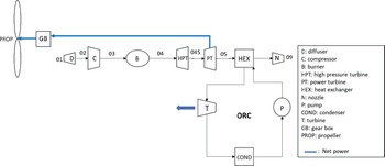
The turboprop engine has almost the same configuration as a turbofan engine. The thermodynamic cycle that describes the operation of the engine is the well-known Brayton cycle. The main difference between a turboprop and a turbofan engine is that the propeller of the turboprop engine is not shrouded, thus imposing a technological limit on its rotational speed. If the propeller’s tip speed were to reach the speed of sound, shockwaves would be generated, severely affecting the engine’s efficiency. Therefore, to avoid this phenomenon, the highest speed that a turboprop aircraft can travel is around Mach 0.7. Because of the absence of a shroud on turboprops, the engines are lighter, which leads to better power-to-weight ratios compared with a turbofan. As far as fuel consumption is concerned, turboprops are more efficient at lower speeds, but they are noisier than turbofans since the propeller is exposed to the atmosphere. For these reasons, turboprop aircrafts are used mainly for shorter-range flight missions, for military purposes as well as cargo transportation. However, turboprops are still an important means of aviation transportation, and some of their advantages compared with turbofans cannot be overlooked.(Reference Sohret, Kincay and Karakoc12) As mentioned above, these engines are suitable for heat recovery since no significant amount of thrust is generated by the exhaust gases. They are generally smaller with a high power-to-weight ratio. This makes it easier to test innovative projects based on them by adding new components to the engine, such as batteries or, in this case, ORC components. A brief description of the engine’s operation is as follows: Air flows through the intake, is compressed through a number of compressor stages and is then mixed with fuel. The high-pressure air–fuel mixture ignites in the combustion chamber to produce high-enthalpy exhaust gases, which are then expanded through a series of turbines to generate the shaft power. The High-Pressure Turbine (HPT) drives the compressor, and the Power Turbine (PT) drives the propeller, which provides most of the engine’s thrust by pushing a large amount of air. In Fig. 1, the flow diagram of a turboprop engine configuration combined with an ORC is presented.

Figure 1. A flow diagram for the whole system.
1.2 Brayton cycle analysis
1.2.1 Reference engine and flight conditions
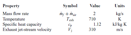
Initially, a simple thermodynamic model is developed without considering the ORC, to calculate the main thermal and physical properties of the engine’s exhaust gas such as temperature, pressure, mass flow rate and specific heat capacity. This is done by selecting a reference engine. The engine drives a small 19-passenger aircraft with a maximum take-off weight of 6,500kg and maximum cruise speed of 115m/s. The engine’s characteristics measured at sea level are presented in Table 1.
Table 1 Reference engine’s basic characteristics
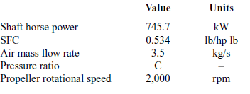
The analysis for both the Brayton cycle and the ORC cycle was derived by assuming steady-state conditions in cruise mode. The flight altitude was selected to be 20,000ft. The flight speed was considered to be the aircraft’s maximum cruise speed of 115 m/s or approximately Mach 0.35. According to the engine’s operational map, these flight conditions correspond to SHP of 500kW and fuel consumption of 0.042kg/s. To continue the analysis, several assumptions had to be made: The air was considered to be an ideal gas. The compressor bleed air and the power necessary to drive the auxiliary systems of the aircraft were neglected for simplicity, since these quantities barely affect the overall behaviour of the engine. The fuel’s Lower Heating Value (LHV) is taken to be 43.2MJ/kg. The values of the specific heat c p and the specific heat ratio  $ \gamma $ were selected for each component separately since they are functions of the air–fuel ratio and the temperature. The c p value ranges from 1.005 to 1. kJ/(kg K), while the value of
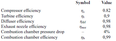
  $ \gamma $ ranges from 1.32 to 1.4. The rest of the assumptions regarding the efficiencies of each individual component are presented in Table 2.
Table 2 Assumed component efficiencies
Most of the data available for the engine were obtained from a sea-level test. Consequently, the thermodynamic properties of the cycle were first calculated for sea-level altitude. Generally, all the engine variables can be described as functions of the atmospheric pressure and temperature, (p a, T a), the flight speed (V) and the fuel mass flow rate (m f). Aircraft engines are designed to operate the same way under different conditions. This means that several dimensionless numbers such as the dimensionless mass flow rate or the ratio between the highest and lowest temperature of the cycle remain constant for the same nondimensional operating point of the engine.(Reference Cumpsty13) As a result, engineers can easily calculate the thermodynamic and aerodynamic properties of a given engine at any altitude even data are available for only one.
1.2.2 Methodology and equations
The approach that was followed was a step-by-step calculation of the thermodynamic properties for each component.(Reference Bali and Hepbasli14) The working fluid of the turboprop engine is taken to be an ideal gas, which is a good approximation for the pressure and temperature levels that occur in this application. The equations for each component of the engine are well known and are thus not presented in this section. However, they are presented as eq. (1-20) in the Appendix for the interested reader and to compare results. The whole set of equations was solved for sea-level conditions as mentioned above, then using the non-dimensional variables of the engine, the analysis was performed for an altitude of 20,000ft as well. For the same non-dimensional operating point of the engine, the dimensionless mass flow rate and the ratio between the highest and lowest temperature of the cycle were considered to remain constant. Using these dimensionless variables, the combustion chamber temperature at 20,000ft was defined, as well as the air mass flow rate. Having all the variables needed for the engine cycle analysis at altitude, the results were then derived.
1.2.3 Results
The results from the thermodynamic analysis of the turboprop engine are summarised in Tables 3 and 4
Table 3 Total pressures and temperatures, sea-level analysis
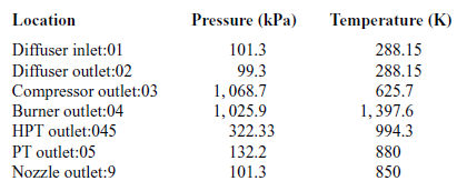
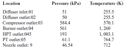
Table 4 Total pressures and temperatures at 20,000ft
During a static ground test of the engine, the flight speed is equal to zero, thus the total temperature at the diffuser inlet is equal to the atmospheric temperature ( $T_{a}=T_{01}$).
Tables 3 and 4 present the pressures and temperatures of each component of the engine. The Temperature-Entropy diagram of the reference engine at 20000ft flight is shown in Fig. 2. The aim is to help the interested reader to understand the ‘identity’ of the engine that is investigated. Moreover, the design and optimisation of the ORC components strongly depend on the characteristics of the engine. These data will aid any potential future research on the same topic as well as comparisons between such results for different types of engine.
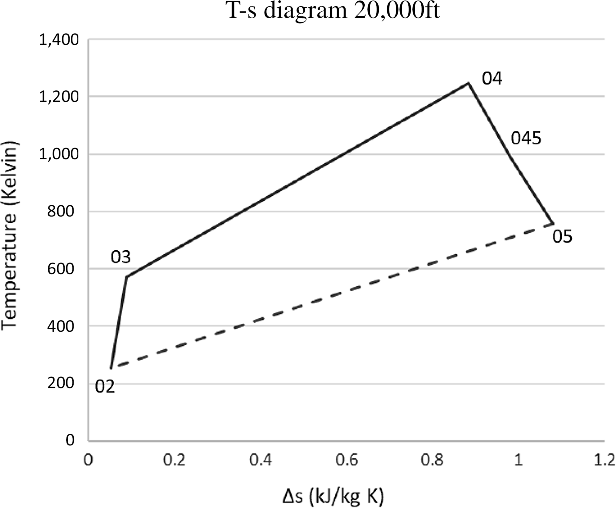
Figure 2. The derivation of the Brayton cycle for the engine.
Having completed the thermodynamic analysis of the engine, the characteristics of the exhaust gases which represent the heat source for the ORC are defined and summarized in Table 5.
Table 5 Exhaust gas characteristics
The thrust produced by the engine is equal to the sum of the thrust produced by the propeller and the thrust produced by the jet stream passing through the engine:
eq. (21).
For steady level flight at constant speed, one can state that the engine’s thrust equals the drag, while the lift equals the weight. The weight was considered to be 6,000kg, slightly less than the Maximum Take-Off Weight (MTOW), and the lift-to-drag factor was assumed to be  $ L/D \approx 11$, a typical value for a turboprop aircraft. Therefore,
  $ F = D = L/11 = W/11 \approx 5350N$.
The thrust produced by the exhaust jet stream from the two engines is 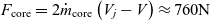 ${F_{{\rm{core}}}} = 2{\dot m_{{\rm{core}}}}\left( {{V_j} - V} \right) \approx 760{\rm{N}}$. This confirms the statement above that the exhaust jet stream provides a small proportion of the total thrust compared with the propeller, in this particular case 14%.
1.3 ORC cycle analysis
1.3.1 Working fluid selection
Much research has been carried out to highlight the best possible working fluid for each application in literature.(Reference Chen, Goswami and Stefanakos15) Different types of refrigerants and hydrocarbons are most commonly used. High latent heat and density, an ‘‘isentropic’’ saturation vapor curve (ds/dT = 0), chemical stability at high temperatures, low freezing point, low environmental impact and safety (a non-flammable, non-corrosive fluid) are the desired characteristics for an ORC working fluid. Aviation applications are sensitive to the addition of extra weight. To avoid carrying another fluid for ORC purposes, which would add complications regarding weight, storage, and piping systems, the concept herein is to use the engine fuel which is already present. By using the engine fuel, we also take advantage of the fact that no further environmental burden is imposed, since the fuel was meant to be used in the combustion chamber anyway. Jet fuel additives ensure that the freezing point is low enough for it to be carried at high altitudes. All of the mentioned desired characteristics for an ORC working fluid are satisfied be the engine fuel to a good degree. The only apparent issue is its high flammability. A sensitivity analysis to determine the optimal operating pressures for the current application was performed, the goal being to maximise the power produced by the organic cycle while considering safety issues and avoiding the auto-ignition temperature of kerosene. This cycle analysis requires that the thermodynamic characteristics of the engine fuel be determined. Aviation fuel is a mixture of different carbohydrates, generally consisting of 79% alkanes, 20% aromatic carbohydrates, and 1% olefins by volume. The average chemical formula of the jet fuel is C12.5H24.4 with a molar mass of 175g/mole.(Reference Goodger and Vere16) Its boiling point at normal conditions ranges from 144 to 252°C. It is notable that jet fuel evaporates at higher temperatures than water but has a significantly lower enthalpy of vaporisation (207kJ/kg at 37.8°C) compared with the value of approximately 2,560kJ/kg for water. This means that it can evaporate more easily from a lower-grade heat source since the energy required for a fluid to evaporate is the sum of the heat necessary to reach the evaporation temperature and the heat required for the isothermal phase change process. The mixtures used in jet fuel have to meet certain specifications, but they are not always the same. This means that the thermodynamic properties of jet fuels may vary, and it is not easy to obtain the corresponding thermodynamic tables. Decane (C10H22) is often used as a surrogate fuel for aviation fuels since it has similar thermodynamic and combustion characteristics. In this work, a mixture consisting of 78% n-decane (C10H22), 12.2% toluene (C7H8) and 9.8% cyclohexane (C6H12) was selected as a substitute for the jet fuel. This mixture is based on Cathonet’s approach(Reference Zeng, Liang, Li and Ma17) and is more accurate one than using just decane as a surrogate fuel for kerosene. The specific heat capacity of the fuel is among the most important properties for this application since it determines in an important way the power produced by the ORC and the necessary heat input rate. The c p value of the surrogate fuel ranges from 1.7 to 2.7kJ/kg K depending on the fluid’s temperature and phase. The results were validated from ref. (Reference Rupprecht and Faeth18). Having determined the working fluid for the ORC, the simulation of the ORC could proceed.
1.3.2 ORC simulation
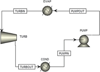
An ORC configuration was designed in thermodynamic analysis software.(19) As shown in Fig. 3, the evaporator heat duty and the power produced by the cycle are the main quantities to be calculated. To achieve this, the operational point of the cycle (pressures and temperatures) and the working fluid mass flow rate must be determined. Any Rankine cycle operates between two pressures: the high pressure at the pump outlet, which is the pressure at which the working fluid evaporates, and the low discharge pressure of the turbine, which is the pressure at which the fluid condenses. These pressures determine the temperatures the fluid must reach to evaporate or condense. Generally, the higher the pressure, the higher the evaporation or condensing temperature. The auto-ignition temperature of kerosene is 210°C at normal conditions. The surrogate fuel evaporates at 210°C at a pressure of 2.3bar. Thus, to avoid this temperature, the highest possible pressure of the cycle should be below 2.3bar. The auto-ignition temperature of the fluid can be surpassed if it can be ensured that no air will infiltrate the ORC system, which means that the lowest pressure of the ORC should be higher than the external atmospheric pressure (0.46bar at 20,000ft). Both of these options for ensuring safety hinder the potential of the cycle to produce more power. To determine which option is better and the exact values of the operating pressures, a sensitivity analysis was performed with the objective of maximising the power.
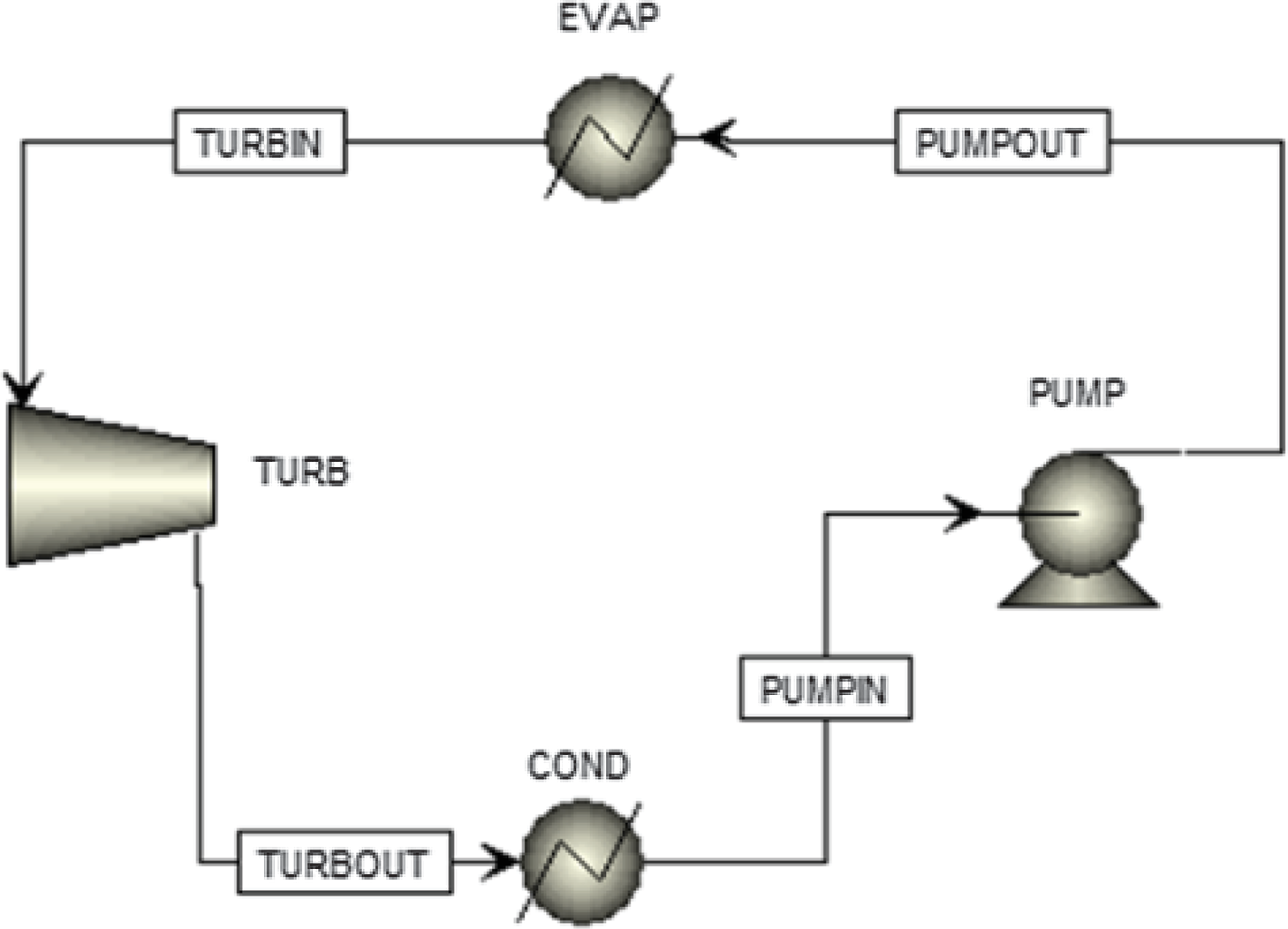
Figure 3. The ORC simulation.
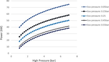
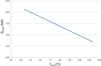
Figure 4 shows that it is more favourable to achieve low condensing pressures than to have evaporation pressures above 2.3bar and a relatively high condensing pressure. A rule of thumb to increase the work produced in any Rankine cycle is to have the highest value possible for the high pressure of the cycle, and the lowest value possible for the low pressure. This is confirmed by the sensitivity analysis of the ORC. The highest power of around 38kW could be achieved for the given range of evaporator pressures (1–7bar) and a condenser pressure of approximately 0.5bar. On the other hand, when avoiding the auto-ignition temperature by decreasing the high pressure to 2bar but keeping the low pressure of the cycle at 0.05bar, a greater amount of power of around 50kW can be obtained by the ORC. Aside from safety issues, an upper limit on the power generation by the cycle is the theoretical maximum heat that can be transferred from the exhaust gases to the fuel in order for it to evaporate. In this case, this amount of energy is a function of the hot exhaust gas inlet temperature in the heat exchanger (working as an evaporator) and the cold fuel inlet temperature. In particular, when two fluids exchange heat, one can write $\;{\dot Q_{{\rm{max}}}} = {\left( {\dot m{c_p}} \right)_{{\rm{min}}}}{\rm{\Delta }}{\rm T}$. In a phase change process, one can assume
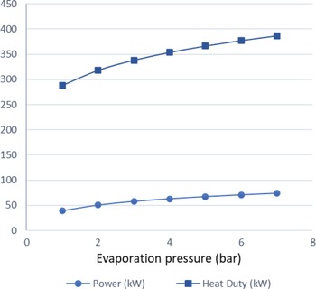
  ${\left( {\dot m{c_p}} \right)_{{\rm{min}}}} \ll {\left( {\dot m{c_p}} \right)_{{\rm{max}}}}$ where the maximum value corresponds to the fluid that changes phase. Therefore, we can define the maximum heat that can be transferred using eq. (22). Both increasing the evaporation pressure and decreasing the condensing pressure of the cycle lead to an increased heat duty of the evaporator. This is another benefit of having lower condensing pressures in the cycle, because although the demand for heat becomes greater, there is an simultaneous increase in the theoretical maximum heat flow that can be transferred, which means that an efficient heat exchanger could achieve the task. Regarding the mass flow rate of the ORC working fluid, there is a trade-off between producing high power and the heat duty of the evaporator. We want to keep the mass flow rate as low as possible so that the whole ORC system remains compact. A mass flow rate of 0.5kg/s was selected by using a trial-and-error approach to obtain a sufficient amount of power while keeping the required heat for the organic cycle relatively low. The calculations shown in Fig. 6 were carried out using this mass flow rate of 0.5kg/s. In Fig. 5, it can be seen that, for an evaporation pressure equal to 2bar, we need a heat input in the cycle slightly above 300kW. Figure 6 demonstrates the theoretical maximum amount of heat that one can extract from this energy source, i.e., the exhaust gas of the turboprop engine. Using these data, we can calculate the heat exchanger efficiency required to exploit the desired amount of heat. The heat exchanger efficiency is defined as the ratio between the actual heat flow transferred and the maximum heat that can be transferred as described in eq. (23). The final operating conditions of the ORC that are chosen based on the results of the sensitivity analysis above, are shown at Table 6.

Figure 4. Sensitivity analysis of the ORC to determine the pressures of the cycle.
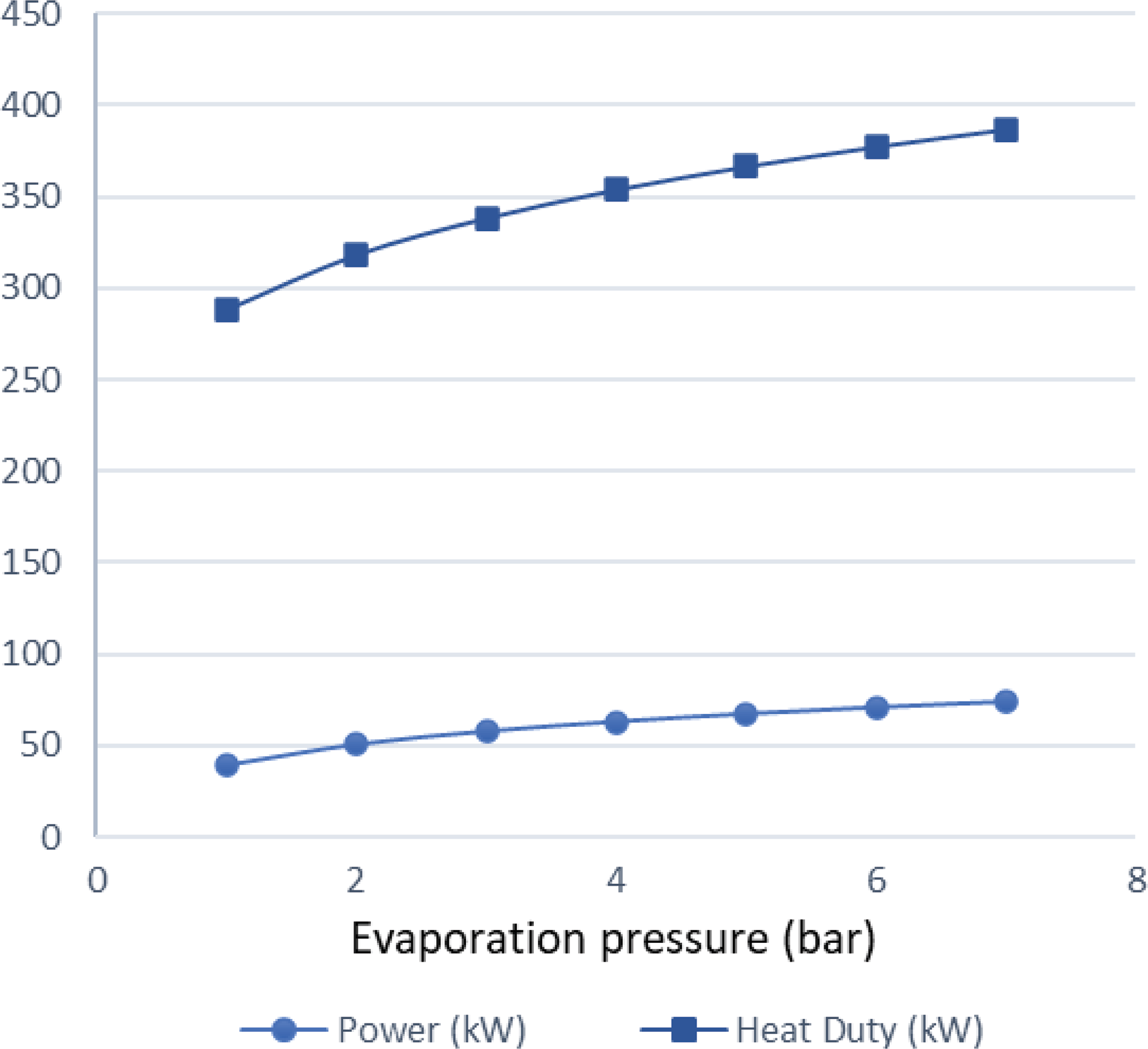
Figure 5. Heat duty and power produced versus evaporation pressure.

Figure 6. Maximum theoretical heat flow that can be transferred from the exhaust gases to the fuel for different condensation temperatures.
Table 6 ORC operating conditions

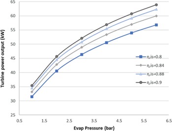
Generally, ORCs are not very efficient due to the low heat source temperature level. Therefore, optimisation of an ORC system usually means maximising the output power of the cycle, as occurs in this case. This also means that the total efficiency of the ORC is very sensitive to the efficiency of each of its components. The proposed ORC has a cycle efficiency of 15.15%, considering both an ideal turbine and pump. The turbine is considered to be the more crucial component in the ORC design. Therefore, an investigation of the effect of its technology level on the cycle was carried out. The isentropic efficiency of the turbine is a good indicator of its technology level, and seem in Fig. 7, it strongly affects the power output of the cycle.
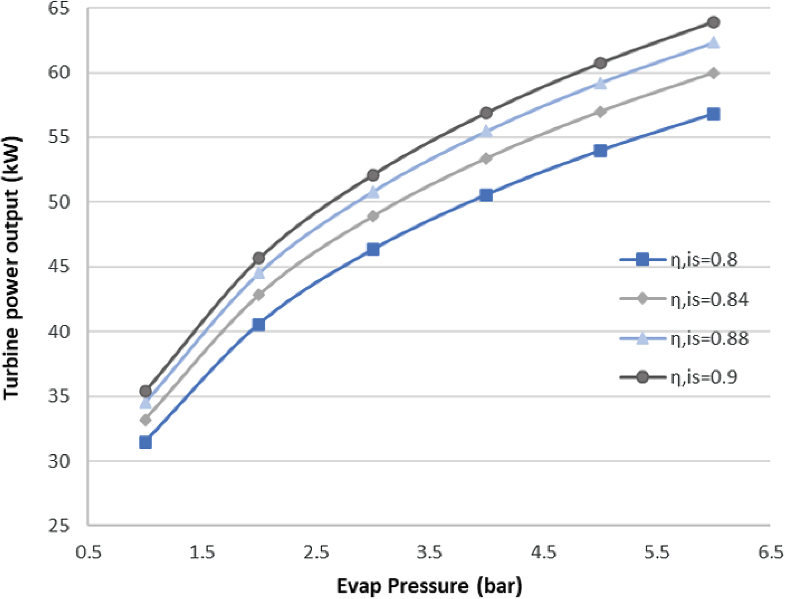
Figure 7. Sensitivity analysis for the ORC turbine.
As seen here, for an evaporation pressure of around 2bar, we obtain a range of power output from 41 to 47kW for different isentropic efficiencies. In other words, a 0.1 increment in the isentropic efficiency of the turbine leads to an approximately 15% increase in the output power. In the results presented below, the turbine isentropic efficiency is taken to be the best possible for the current state of the art, with a value of 0.9.
1.3.3 Results
Having determined the operational conditions of the ORC, the results of the cycle simulation are now demonstrated at Table 7.
Table 7 ORC simulation results

The ORC simulation was performed with both the selected surrogate fuel and n-decane as working fluid. The results are more favourable with the surrogate fuel since it has a lower condensation temperature (43.6°C) due to its lower specific heat capacity compared with decane. Despite this, the results are quite similar with approximately 50kW of power produced, leading to an increase of the thermal efficiency of the engine by 10.1%. The power required by the pump is around 0.5kW. This value corresponds to 1% of the power produced from the turbine and can therefore be neglected. The heat exchanger (evaporator) efficiency ε required to satisfy the heat demand of this cycle is around 0.4. The T–s diagrams of the working fluids are shown in Figs 8 and 9.

Figure 8. The temperature–entropy diagram of the ORC with decane as a working fluid: 1-2, pump; 2-3, evaporator; 3-4, turbine; 4-1, condenser.

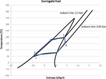
Figure 9. The temperature–entropy diagram of the ORC for the surrogate fuel.
In Fig. 9, the isothermal lines are not parallel to the x-axis. This occurs because the fuel substitute consists of three different fluids with different boiling points. Therefore, when one of the components reaches its evaporating temperature, the others may not and are still contributing to increase the temperature of the mixture. The need for an efficient heat exchanger could potentially mean that a large heat exchanger should be part of the ORC, resulting in geometrical characteristics that do not match the small turboprop engine or extra weight that will hinder the performance of the engine. This difficulty can be overcome by utilising modern techniques for designing compact heat exchangers with large heat transfer area-to-volume ratio. The current state of the art is around 6,000m2/m3 for compact glass–ceramic heat exchangers for use in gas turbine applications.(Reference Cengel and Ghajar20) Nevertheless, there is some margin to decrease the power produced by the ORC and consequently the heat duty of the evaporator, thus reducing its size, while still obtaining significant results.
1.4 Heat exchanger 0-D design
As seen from the discussion above, the heat exchanger is one of the most crucial parts of this project since it connects the two thermodynamic cycles. A zero-dimensional (0-D) tool was developed to calculate the approximate heat exchange area required to transfer the necessary amount of heat to the ORC. The NTU method was used for the calculations. The NTU is given by eq. (24). Generally,  $\varepsilon$ is a function of NTU and c, which is calculated from eq. (25). In a phase change process, as mentioned above,
 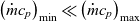 ${\left( {\dot m{c_p}} \right)_{{\rm{min}}}} \ll {\left( {\dot m{c_p}} \right)_{{\rm{max}}}}$, thus
  $c \approx 0$ and
  $\varepsilon$ is dependent only on NTU, as shown in eq. (26). In our case, the value of ε is known from eq. (23). We can then calculate the NTU from eq. (26). Consequently, in eq. (24), the only unknowns are the heat transfer coefficient h and the required exchanger area A s. Calculating the heat transfer coefficient is the next step. An appropriate type of heat exchanger for the application would be a compact fin-and-tube design with fins on the side of the gas to enhance the total heat transfer coefficient. A simplified sketch of a fin and tube heat exchanger is shown on Fig. 10. The tube diameter and arrangement are crucial factors to achieve an efficient heat exchanger design.(Reference Salpingidou, Misirlis, Vlahostergios, Flouros, Donnerhack and Yakinthos21,Reference Salpingidou, Misirlis, Vlahostergios, Flouros, Donnerhack and Yakinthos22) The choice of the heat exchanger material is another important factor that should be considered. Low density, high thermal conductivity, high melting point and resistance to corrosion are the most important characteristics to consider. Aluminium is a great choice since it satisfies all of the above characteristics adequately. Its only drawback is its relatively low melting point (933K). For this work, stainless steel was selected, even though it is considerably denser (7,950kg/m3) compared with aluminium (2,700kg/m3) and has a lower thermal conductivity of 15W/(m K) compared with 237W/(m K) for aluminium. This choice was made to ensure safe operation of the heat exchanger. The exhaust gases have a lower mean temperature (600K) than the melting point of aluminium, but locally the temperature could reach higher values. Also, the calculations were carried out for cruise mode. At a different operating point of the engine, the temperature values may be even higher, causing significant thermal stresses on the heat exchanger. Stainless steel has a melting point of around 1,670K, which is more than sufficient to ensure the safety and long-term operation due to its corrosion resistance.

Figure 10. Flow around the tubes of a fin-and-tube heat exchanger.
The total heat transfer coefficient for a flow around a cylindrical tube is given by eq. (27), where “in” refers to the inner flow of the pipes (ORC working fluid) and “out” refers to the outer exhaust gas flow. This equation can be simplified greatly if the tube’s wall is thin enough that its dimensions become negligible compared with its diameter, and the material from which the tube is constructed has a high conductivity coefficient. This is true in most cases. Therefore, we can neglect the second term in eq. (27). Also, in this case, the inner fluid is a phase changing liquid while the outer fluid is a gas. One can then safely assume that  ${h_{{\rm{in}}}} \gg {h_{{\rm{out}}}}$, finally yielding
  $ U \approx h_{out}$. To calculate U, we must first calculate the Nusselt number, which is a function of Pr and Re. The most common correlation used to calculate the Nusselt number for a flow around cylindrical tubes is the Zakaus(Reference Cengel and Ghajar20,Reference Salpingidou, Misirlis, Vlahostergios, Flouros, Donnerhack and Yakinthos21) correlation described in eq. (28), where C, m and n are constants depending on the Reynolds number. All of the properties necessary for the Nusselt calculation except Prs were defined at the mean temperature of the exhaust gas stream, which is estimated to be 360°C. The flow is governed by the maximum velocity that occurs between the pipes. The Reynolds number in eq. (28) is calculated using this velocity and the diameter of the pipes. The maximum velocity between the pipes is calculated as follows: if
 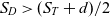 $S_{D} \gt (S_{T} + d)/2 $ then the maximum velocity between the tubes is calculated from eq. (29). Otherwise, eq. (30) is used. After calculating Nu, we can obtain the heat transfer coefficient value from the definition of the Nusselt number:
  $ Nu = \frac{hd}{k}$
Finally, the required area of heat exchanged can be estimated from eq. (24). Figure 11 illustrates the heat exchange area required for different achieved values of the heat exchanger’s total heat transfer coefficient. As expected, the higher the heat transfer coefficient, the smaller the area required for heat exchange, thus a more compact heat exchanger design can be achieved. The pressure drop imposed by the heat exchanger on the exhaust jet stream of the aircraft is calculated from eq. (31). The friction factor f and the correction factor χ both depend on the Reynolds number plus the tube diameter and arrangement. As stated above, the thrust provided by the exhaust nozzle is low compared with the propeller thrust, thus the main constraint for the pressure drop is the need to exhaust the flow in an aerodynamically correct way. The pressure of the exhaust gases after the heat exchanger should be larger than atmospheric. From the turboprop engine analysis (Table 4), the maximum allowed pressure drop before we reach the atmospheric pressure is around 15kPa, or up to 23% in percentage terms. In the calculations for the heat exchange design, the pressure drop was fixed at 6kPa (10% pressure drop) so that the appropriate geometrical characteristics and number of tubes could be found.
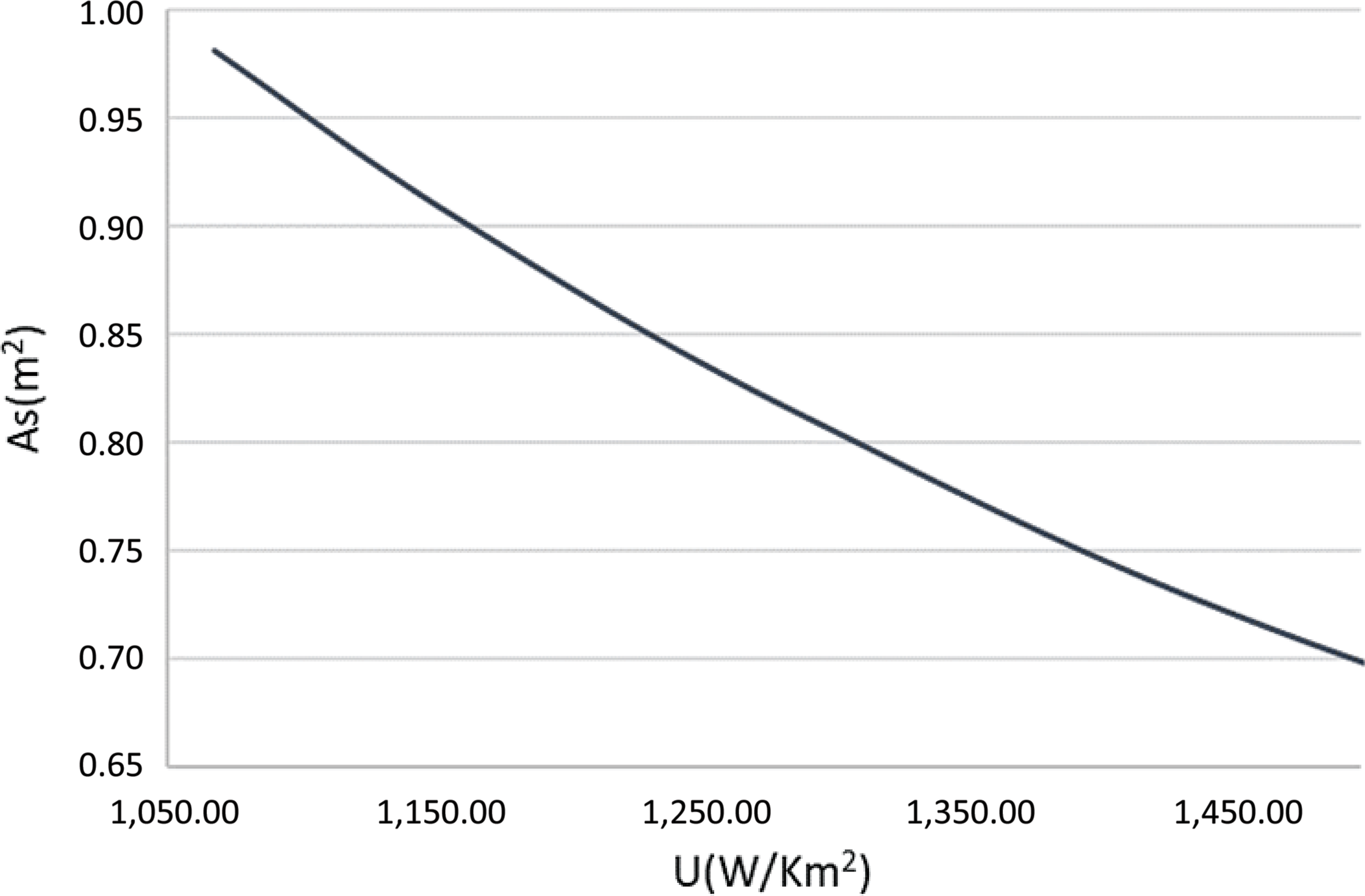
Figure 11. Heat transfer coefficient versus heat exchange area.
Different solutions for different tube diameters and arrangements were derived using the computational tool that was developed, so that the best combination of the heat exchanger’s total heat transfer coefficient and weight was achieved. The number of tubes and the distances between them were selected such that the size limitations of the aircraft’s exhaust duct were respected. The results are summarised in Table 8. The lowest possible heat exchange area was calculated to be slightly more than 2m2. Since this is a 0-D analysis, the exact geometry of the heat exchanger is not defined, thus its area-to-volume ratio is not known. The heat exchanger’s surface-to-volume ratio was assumed to be a conservative 1,500m2/m3, which is an achievable value for a compact fin-and-tube heat exchanger.(Reference Cengel and Ghajar20)
Table 8 Heat exchanger characteristics for different cases

From the results above, it is notable that, the denser the tube arrangement, the higher the total heat transfer coefficient. The disadvantage of using a dense tube configuration is that the maximum velocity of the exhaust gas flow increases and the pressure drop of the exhaust stream is proportional to the square of the maximum velocity. The pressure losses also increase in proportion to the number of tubes that are set in the flow direction. With higher velocity values, the number of tubes allowable in the flow direction decreases so that the pressure losses remain at 3kPa. To reach a compromise with fewer tubes, which means a smaller heat exchange surface, the percentage of the finned area must be increased. The weight of the exchanger is calculated to be around 3% of the total engine weight (175kg). The use of a less dense material as well as a heat exchanger with a sophisticated design to achieve a large area density (m2/m3) would further decrease the weight.
2.0 CONCLUSIONS
The research presented herein focuses on heat recovery from aircraft engine exhaust gases by using an ORC system to generate power. In particular, the engine that is investigated is the Honeywell TPE 331-10 turboprop engine. The main conclusions of the proposed concept can be summarised as follows:
-
• Turboprop engines are suitable for heat recovery since most of the thrust is provided by the propeller.
-
• A safe ORC as far as flammability is concerned with the jet fuel as a working fluid can be designed and still provide significant results in terms of the power generated by the cycle.
-
• Low condensing pressures are more favourable than high evaporation pressures for this application, since the lower the condensing temperature, the higher the work produced by the cycle as well as the theoretical maximum heat flow that can be transferred from the exhaust gases to the ORC working fluid.
-
• A surrogate for aviation fuel that is satisfactory in terms of having similar properties can be obtained by using simpler chemical compounds whose thermodynamic and physical characteristics are known.
-
• The results show that the design of an evaporator that meets the weight and size limitations of an aircraft while providing sufficient heat to the ORC working fluid is possible.
-
• Future work should focus on a detailed design for a compact heat exchanger with the above desired characteristics.
-
• By integrating an ORC system into the turboprop engine, a subsequent snowball effect occurs. The extra 50kW of power produced by the ORC means that the engine could use less fuel to produce the same power, but less fuel means lower exhaust gas temperatures, which would hinder the performance of the ORC.
-
• Alternatively, the extra power generated by the ORC could be applied directly to the turbine shaft, which would mean that a larger propeller could be adapted to the shaft, resulting in more thrust produced by the engine. This again leads to a snowball effect because more thrust would mean a change in the aerodynamic characteristics of the aircraft and also a potential change at the design point of the turboprop engine. To avoid this, the authors suggest simply adjusting the existing propeller’s angle so that a greater air mass flow could be pushed.
-
• The integration of an ORC system with the suggested operating conditions toin the turboprop engine leads to an increasement of the engine’s thermal efficiency by 10.1%.
APPENDIX
 \begin{equation}p_{01} =\frac{1}{2} \rho V^{2} +p_{{\rm a}}\end{equation}
 \begin{equation}T_{01} =\frac{V^{2} }{2c_{p} } +T_{{\rm a}}\end{equation}
 \begin{equation}p_{02} =\eta _{dif} p_{01}\end{equation}
 \begin{equation}T_{01} =T_{02}\end{equation}
 \begin{equation}T_{03is} =T_{02} \pi ^{(\gamma -1)/\gamma }\end{equation}
 \begin{equation}\eta _{c} =\frac{T_{03is} -T_{02} }{T_{03} -T_{02} }\end{equation}
 \begin{equation}p_{04} =p_{03} \times (1-0,04)\end{equation}
 \begin{equation}{\eta _b}{\dot m_f}LHV = \left( {{{\dot m}_{air}} + {{\dot m}_f}} \right){c_p}\left( {{T_{04}} - {T_{03}}} \right)\end{equation}
 \begin{align}{\dot{m}}_{air}c_{p,air}\left(T_{03}-T_{02}\right)= ({\dot{m}}_{air}+{\dot{m}}_f)c_{p,gas}\left(T_{04}-T_{045}\right)\end{align}
 \begin{equation}T_{045is} =T_{04} /\left(\pi _{HPT} ^{(\gamma -1)/\gamma } \right)\end{equation}
 \begin{equation}\eta _{t} =\frac{T_{04} -T_{045} }{T_{04} -T_{045is} }\end{equation}
 \begin{equation}{{\rm SHP} =\ }\left({\dot{m}}_{air}+{\dot{m}}_f\right)c_{p,gas}\ \left(T_{045}-T_{05}\right)\end{equation}
 \begin{equation}T_{05is} =T_{045} /\left(\pi _{PT} ^{(\gamma -1)/\gamma } \right)\end{equation}
 \begin{equation}\eta _{t} =\frac{T_{045} -T_{05} }{T_{045} -T_{05is} }\end{equation}
 \begin{equation}p_{09} =\eta _{noz} p_{05}\end{equation}
 \begin{equation}T_{09} =T_{05}\end{equation}
 \begin{equation}\frac{p_{05} }{p_{{\rm a}} } =({{\rm T} _{05} \mathord{\left/ {\vphantom {{\rm T} _{05} {\rm T} _{9} )}} \right.} {\rm T} _{9} )} ^{\gamma /(\gamma -1)}\end{equation}
 \begin{equation}V_{jet} =\sqrt{2c_{p,exh} (T_{05} -T_{9} )}\end{equation}
 \begin{equation}\frac{{\dot{m}}_{air}\sqrt{T_{02}}}{p_{02}}=const\end{equation}
 \begin{equation}T_{04} /T_{02} =const\end{equation}
 \begin{equation}F=F_{prop} +F_{core}\end{equation}
 \begin{equation}{\dot{Q}}_{max}={\dot{m}}_{core}c_{p,exh}(600-T_{cond})\end{equation}
 \begin{equation}\varepsilon=\frac{{\dot{Q}}_i}{{\dot{Q}}_{max}}\end{equation}
 \begin{equation}NTU=UA_s/(\dot{m}c_p)_{min}\end{equation}
 \begin{equation}c=({\dot{m}c_p)}_{min}/({\dot{m}c_p)}_{max}\end{equation}
 \begin{equation}\varepsilon =1-e^{-NTU}\end{equation}
 \begin{equation}\frac{1}{UA_{s}} =\frac{1}{h_{out} A_{out} } +\frac{\ln ({d_{out} \mathord{\left/ {\vphantom {d_{out} d_{in} )}} \right.} d_{in} )} }{k_{wall} 2\pi L} +\frac{1}{h_{in} A_{in} }\end{equation}
 \begin{equation}Nu=C\,\text{Re}_{,d}^{m}\ \text{Pr}^{n} (\text{Pr}/\text{Pr}_{s})^{0,25}\end{equation}
 \begin{equation}V_{\max } =S_{T} V_{exh} /(S_{T} -d)\end{equation}
 \begin{equation}V_{\max } =S_{T} V_{exh} /2(S_{D} -d)\end{equation}
 \begin{equation}\Delta P=N_{L} f\chi \frac{\rho V_{\max }^{2} }{2}\end{equation}


 Open access