2.1 Geometry and computational setup for ground effect

The geometry for the CRM-WB-HL configuration is an extension of the CRM wing-body geometry [Reference Vassberg17] also used in the Drag Prediction Workshop [20]. The CRM wing consists of a thin supercritical aerofoil with an aspect ratio of $AR{\rm{\;}} = {\rm{\;}}9$ and a taper ratio of $0.25$ . The high-lift configuration CRM [Reference Lacy and Clark16] that is used in this paper to estimate the ground effect is the nominal configuration provided by the High-Lift Prediction Committee in HLPW 4 [18]. The CRM-WB-HL configuration is shown in Fig. 1.

The high-lift CRM wing has the same geometrical features as the CRM wing-body configuration, with mean aerodynamic chord $c = 7.0{\rm{m}}$ , wingspan $b = 58.76{\rm{m}}$ and reference area ${S_{ref}} = 383.65{{\rm{m}}^2}$ . The inboard and outboard flaps are deflected by ${40^ \circ }$ and ${37^ \circ },$ respectively, and the slat is deployed by ${30^ \circ }$ . Table 1 shows important reference parameters for the CRM-WB-HL configuration that was employed in this study. The original computer-aided design (CAD) model and additional geometry information are available at Refs. [Reference Lacy and Clark16, 18, Reference Evans, Lacy, Smith and Rivers21].

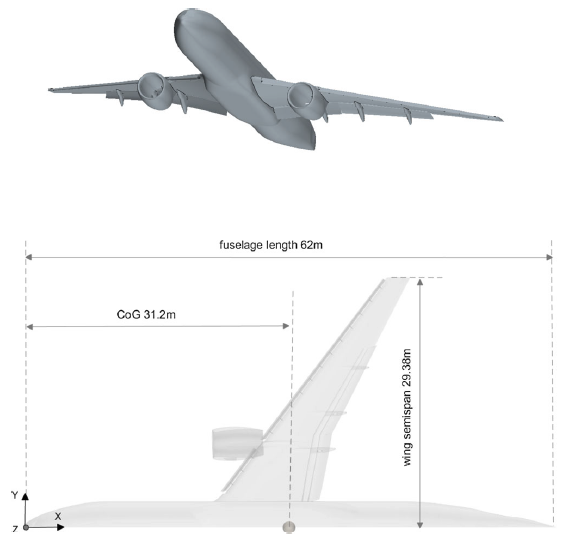
Figure 1. Geometry of the full CRM high-lift configuration, isometric view (top) and planform view (bottom).

The computational domain is a virtual wind tunnel in the shape of rectangular box 1,000c away from the aircraft model CoM in every direction, except for the cases of ground effect where the negative $Z$ direction had to be fixed in order to set up the correct non-dimensional ratio $h/c$ defining the closeness to the ground. The usual boundary conditions used in incompressible flow simulations, i.e. the velocity inlet with fixed value boundary condition, and pressure outlet with zero gradient condition at the outlet were employed. For the wind tunnel walls, a slip boundary condition is employed while a no-slip boundary condition was used for the aircraft surfaces. In the case of close proximity to the ground, a prism boundary layer was used and a moving wall boundary condition was allocated with specified relative velocity in order to accurately capture the ground effect. In addition, for investigation of the ground effect, the desired flight attitude is obtained by rotation around the moment reference point given in Table 1. Examples of aircraft positions used to study ground effect aerodynamics with $h/c = 1.0$ , $\alpha = {8.0^ \circ }$ and various roll angles $\phi $ are shown in Fig. 2.

2.2 Governing equations

The Navier–Stokes (NS) equations governing incompressible fluid flow are the continuity and the momentum equations:

(1) \begin{align}\nabla \cdot {\bf{U}} = 0\end{align}

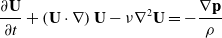(2) \begin{align}\frac{{\partial {\bf{U}}}}{{\partial t}} + \left( {{\bf{U}} \cdot \nabla } \right){\bf{U}} - \nu {\nabla ^2}{\bf{U}} = - \frac{{\nabla {\bf{p}}}}{\rho }\end{align}

where ${\bf{U}}$ is the velocity vector, $\nu $ is the kinematic viscosity of the fluid, ${\bf{p}}$ is the pressure and $\rho $ is the density.

The computational resources required for direct numerical simulations (DNS) of Equations (1) and (2), especially for flow conditions with high Reynolds numbers, usually exceed currently available computational capabilities. Instead the RANS equations are solved, in which the Reynolds stresses arising as a result of averaging the fluctuating velocities are described by some additional empirical equations either algebraic or differential to represent an appropriate turbulence model. Most turbulence models for the RANS equations are based on the concept of eddy viscosity, which is equivalent to the kinematic viscosity of a fluid, to describe turbulent mixing or flow momentum diffusion [Reference Chen, Xiong, Morris, Paterson, Sergeev and Wang22]. Reynolds stresses arising in the RANS equations due to time averaging are described in linear turbulence models under the Boussinesq assumption:

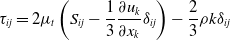(3) \begin{align}{\tau _{ij}} = 2{\mu _t}\left( {{S_{ij}} - \frac{1}{3}\frac{{\partial {u_k}}}{{\partial {x_k}}}{\delta _{ij}}} \right) - \frac{2}{3}\rho k{\delta _{ij}}\end{align}

where ${\tau _{ij}}$ in Equation (3) is the Reynolds stress tensor, ${\mu _t}$ is the turbulent viscosity, ${S_{ij}}$ is the strain rate tensor and $k$ is the kinetic energy.

2.3 Grid generation

Computational grids with an overset meshing approach are generated using the Siemens StarCCM+ software which is well known for its robust overset/chimera methods and simulation capabilities [23]. The reason for relying on self-generated grids rather than directly using the grids provided by HLPW [18] is twofold. Firstly, it allows to modify the flight attitudes by manipulating the overset mesh enclosing the aircraft in close proximity to the ground rather than generating/updating the grid for every new flight attitude. This is necessary as changing the wind velocity vector is not a viable option for the ground effect simulations due to the limited vertical offset distance available between the ground/runway and the velocity inlet boundary. Secondly, the overset grids also gives an opportunity to simulate the dynamic mesh for aircraft oscillatory motions for computation of dynamic aerodynamic derivatives, which is planned for a later stage of this study.

Table 1. Reference data for the CRM-WB-HL (full model)

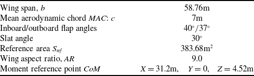
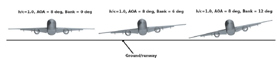
Figure 2. Considered aircraft attitudes for investigation of the lateral-directional aerodynamics in close proximity to the ground at $h/c = 1.0$ and $\alpha = {8.0^ \circ }$ .

The first mesh region is taken as the overset mesh with a close-bound box around the CRM-WB-HL model $2.0{\rm{m}}$ away in every direction, enabling to go for reduced proximity to the ground characterised by the non-dimensional ratio $h/c$ . In the first mesh region, for the boundary layers generated on aircraft surface, a $Y + $ non-dimensional wall distance was chosen at a value of $1$ , as required in the low wall $Y + $ treatment. The second mesh region is the background mesh generated for the wind tunnel/computational domain. Further refinement or body of influence is placed in the wake of the aircraft in both the background mesh and the overset mesh region which allows to refine a region of interest in the volume mesh. Although not strictly required, conformal mesh sizes are used on the overlapping region between the overset box surface and the background mesh interface of both regions. This enables smooth interpolation of conserved flow variables between the two mesh zones. The cell area and volume in the immediate vicinity of this overlapping region or the overset interface region vary by $1-2{\rm{\% }}$ between the two zones, i.e. the overset zone and the wind tunnel mesh. A coarse grid is initially generated with $5$ m elements. This mesh is then scaled to produce more dense and refined grid levels. The resulting computational grids are in the range of $5-94$ m elements. The generated grid for CRM-WB-HL configuration is shown in Fig. 3.

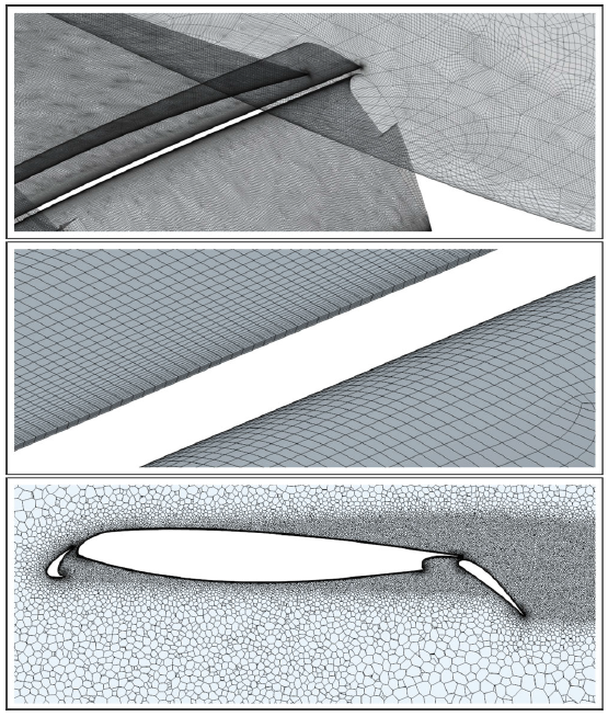
Figure 3. Grid generated for the NASA CRM high-lift configuration, fuselage-wing connection (top), wing and flap junction (middle) and cross-sectional view of the wing (bottom) in OGE conditions.

2.4 Numerical solver settings

The numerical solver settings used in this study reflect changes in flow properties. For small angles of attack with $\alpha \lt {10^ \circ }$ , the steady RANS formulation was used along with the well-known Spalart-Allamaras [Reference Spalart and Allmaras24] turbulence model. At moderate to high angles of attack $\alpha \gt {10^ \circ }$ the simulation was switched to the Unsteady Reynolds Averaged Navier-Stokes (URANS) formulation, as this allows a more accurate prediction of the separation zones and vortex shedding processes.

The continuity, momentum and turbulence equations were solved in a segregated manner using the algebraic multi-grid (AMG) solver with an inner tolerance of $0.001$ instead of the default value of $0.1$ , thus solving the matrix holding the discretised finite volume coefficients to an order of a minimum three orders of magnitude. This setting allows a good convergence for every time step at the expense of slightly increased computational time. The V and F cycle approach was employed with ${\rm{two}}$ pre and post sweeps in order to further maximise convergence. Along with these settings, the AMG restriction tolerance was fixed at $0.9$ and the prolongation tolerance was kept at $0.5$ . It was also necessary to exploit some degree of under-relaxation of the flow variables, especially when modelling the ground effect due to the highly non-stationary nature of the flow field.

Although the grids were intentionally constructed using a low wall $Y + $ approach, i.e. $Y + \lt 1.0$ , Star-CCM+ recommends using All $Y + $ treatment. With this wall treatment method, boundary layers that meets the low $Y + $ criterion are resolved using the low $Y + $ approach, and boundary layers that violate the low $Y + $ criterion are resolved using the high wall $Y + $ treatment method. The gradients of conservative flow parameters are solved with the second order of accuracy along with the Venkatakrishnan limiter [Reference Venkatakrishnan25], which excludes spurious oscillations in the flow field. The SA turbulence model was used with the rotation curvature correction option based on presentations made in Ref. [18] where this approach was shown to give good agreement with the experimental results.

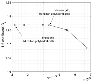
Figure 4. Mesh independence check for OGE simulations: lift coefficient ${C_L}$ at $Re = 5.49 \times {10^6}$ and $M = 0.2$ .

3.1 Mesh independence check

Grid resolution plays an important role in accurately predicting aerodynamic characteristics. The six different grid levels for the CRM-WB-HL configuration were created by scaling the coarsest mesh level with approximately 5m elements. The scaling process was performed by reducing the base mesh size and increasing the resolution in the slat/wing/flap wake regions by specifying the downstream wake length and feature sizes as a percentage of the base size.

The obtained computational results for the mesh independence study at $\alpha = {7.045^ \circ }$ are shown in Fig. 4. The chosen angle-of-attack at $\alpha = {7.045^ \circ }$ is around the trim angle-of-attack for landing configuration which is typically in the range 0–10° for a generic transport airliner (see handling qualities data in Ref. [Reference Heffley and Jewell26], p. 216). The lift coefficient ${C_L}$ obtained for a grid with $16$ m cells is certainly independent of grid resolution, especially at such a low angle-of-attack, and therefore this level of grid resolution was chosen for study in the remaining simulations. A further mesh independence study was also conducted for IGE simulations to reassure our confidence in the chosen level of grid resolution.

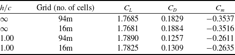
The results of the grid independence study summarized in Table 2 show that at $\alpha = {7.045^ \circ }$ the ${C_L}$ and ${C_m}$ predictions for the OGE and IGE simulations are in good agreement between the $16$ and $94$ m elements. The drag coefficient changes more significantly with increasing grid size compared to the lift and pitching moment coefficients. However, the main focus of this study is on the lift coefficient ${C_L}$ , since the rolling moment generated at the symmetric and asymmetric attitudes of the aircraft depends on the amount of lift produce by the left and right sides of the wing. Based on these results, and to minimise computational cost, a $16$ m mesh is used for further simulations involving ground proximity variation with zero and non-zero bank angles at various normalised height-to-chord $h/c$ ratios from the ground.

Table 2. Mesh comparison for IGE and OGE conditions at $\alpha = {7.045^ \circ }$ for CRM-WB-HL configuration

3.2 Validation against experimental results using medium grid

The computational framework with the SA turbulence model [Reference Spalart and Allmaras24] for the CRM-WB-HL model has been successfully tested against the available OGE data in a wind tunnel at Reynolds number $Re = 5.49 \times {10^6}$ and Mach number $M = 0.2$ (Fig. 5). For this study, the medium grid with a total of $16$ m of elements was used, and the simulations were carried out on the Zeus HPC cluster facility at Coventry University [27].

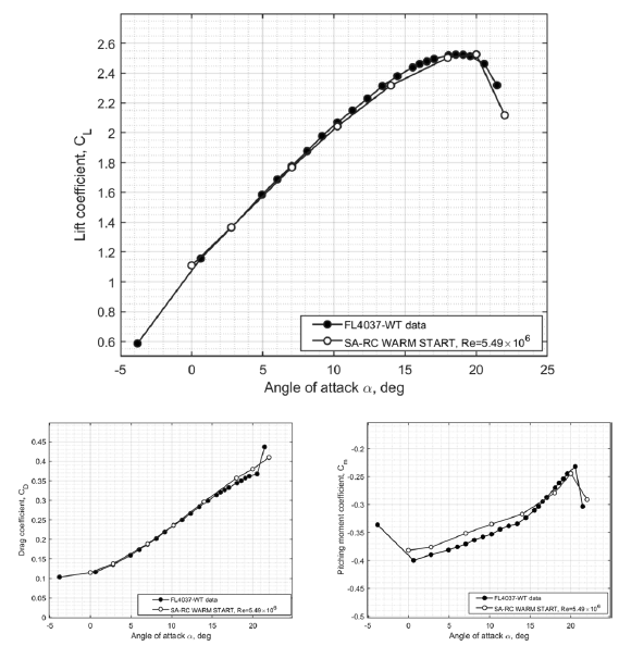
Figure 5. Validation of CFD simulation results against the OGE wind tunnel data at $Re = 5.49 \times {10^6}$ and $M = 0.2$ , experimental results from Ref. [18].

The obtained computational results for the lift coefficient, drag coefficient and pitching moment coefficient are shown against the experimental data from the QinetiQ Five-Meter Pressurized Low-Speed Wind Tunnel FL4037 in Fig. 5. These wind tunnel experimental data are available to download from the HLPW site [18]. The information on the wind tunnel setup and experimental results for the high-lift configuration can be found in Ref. [Reference Evans, Lacy, Smith and Rivers21]. Figure 5 shows that the obtained computational simulation results for the lift coefficient ${C_L}$ and drag coefficient ${C_D}$ are in very good agreement with the experimental data at low angles of attack and in the stall region predicting quite accurately the maximum lift coefficient and the drop in the lift coefficient after the stall [18, Reference Evans, Lacy, Smith and Rivers21]. There is a slight shift for the pitching moment coefficient ${C_m}$ at low angles of attack; however, the general trend in variation of the pitching moment is captured accurately and the stall angle matches with wind tunnel data.

The WARM START simulation method in Fig. 5 refers to a technique in aerodynamic computational simulations where the converged flow field of the previous angle-of-attack’s data is used as the initial solution for the flow field for simulation at a new angle-of-attack. Rather than starting from a non-converged field, the WARM START method allows to continue solution quite effectively. This technique is good for predicting the static hysteresis phenomena because the backward loop can be robustly simulated as well. The transient history of the lift coefficient ${C_L}$ in the OGE simulations using the WARM START method is shown in Fig. 6.

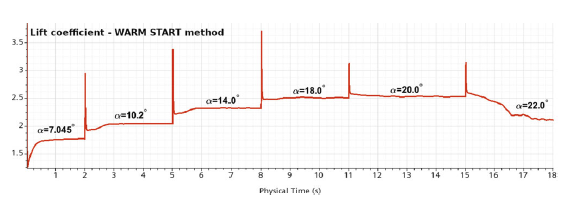
Figure 6. Time history of the lift coefficient ${C_L}$ using the WARM START method for OGE simulations at $Re = 5.49 \times {10^6}$ and $M = 0.2$ .

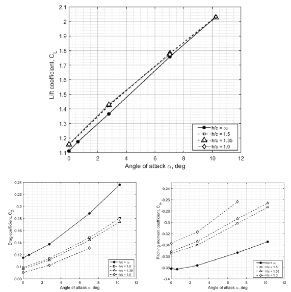
Figure 7. Longitudinal aerodynamic characteristics for IGE simulations at $Re = 5.49 \times {10^6}$ , $M = 0.2$ and flaps inboard $/$ outboard $ = {40^ \circ }/{37^ \circ }$ for $h/c = \infty ,1.5,1.35$ and $1.0$ .

4.1 Ground effect on the longitudinal aerodynamics

The simulation focuses on the analysis of the influence of the ground on the aerodynamic coefficients ${C_L}$ , ${C_D}$ , and ${C_m}$ for various altitude-to-chord ratios. The computational results for various $h/c$ are shown in Fig. 7. At low angles of attack $\alpha \lt {10^ \circ }$ , the maximum positive increment of the lift coefficient ${\rm{\Delta }}{C_L} = 0.055$ occurs at $\alpha = {2.78^ \circ }$ , which is an increment of $4.029{\rm{\% }}$ compared with the value of the OGE. When approaching the ground, more significant changes in the coefficients of drag and pitching moment are observed. As the distance to the ground decreases from $h/c = \infty $ to $h = 1.0$ , there is a significant decrease in the drag coefficient ${C_D}$ and a noticeable positive increase in the pitching moment ${C_m}$ . When comparing the pitching moment coefficient at $\alpha = {7.045^ \circ }$ and $h/c = 1.0$ against $h/c = \infty $ , an increase in the pitching moment coefficient by $25{\rm{\% }}$ takes place. This is a fairly noticeable change in the pitching moment and drag coefficients, which affects both the trim conditions in the longitudinal motion and the characteristics of its stability.

4.2 Ground effect on the lateral-directional aerodynamics

The simulation of the ground effect on the rolling and yawing moment coefficients is carried out by introducing a certain non-zero bank angle. When landing in a crosswind, significant bank angles will occur due to wind disturbance and the need to balance the aircraft with a non-zero bank angle (sideslip approach) [3]. Such aircraft attitudes in close proximity to the ground will induce additional changes in the rolling and yawing moments. A better understanding of flight dynamics, trimming and stability conditions in the case of crosswind landing in close proximity to the ground is an important task from the flight safety point of view [3]. The obtained simulation results for angle-of-attack $\alpha = {8.0^ \circ }$ at $h/c = 1.0$ and for the range of bank angles ${0^ \circ } \le \phi \le {12^ \circ }$ are presented in Fig. 8.

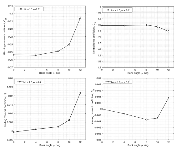
Figure 8. Variation of aerodynamic coefficients against bank angle in IGE simulations at $\alpha = {8^ \circ }$ , $Re = 5.49 \times {10^6}$ , $M = 0.2$ and with deployment of flaps inboard $/$ outboard at $ = {40^ \circ }/{37^ \circ }$ .

The simulation results in Fig. 8 show that the pitching moment coefficient ${C_m}$ quite significantly increases with the bank angle in close proximity to the ground (a nose-up effect). There are very small negative changes in the normal force coefficient ${C_N}$ at bank angles $\phi \gt {8.0^ \circ }$ . For example, at $\phi = {12.0^ \circ }$ a decrease in the normal force coefficient ${C_N}$ is equivalent to a loss of approximately $2.17{\rm{\% }}$ of the normal force. The percentage loss of normal force coefficient is small throughout the right wing, but increases towards the wing tip. Due to the long arm on the wing tip, the small change in the normal force generates a significant contribution to the rolling moment ${C_l}$ . This effect is reflected in the rolling moment coefficient shown in Fig. 8. With the increase of bank angle $\phi $ (the right wing goes towards the ground) the rolling moment coefficient increases from ${C_l} = 0.0$ at $\phi = {0^ \circ }$ to ${C_l} \approx 0.0218$ at $\phi = {12^ \circ }$ . A positive rolling moment ${C_l} \gt 0$ indicates the presence of a suction effect that presses the right wing to the ground. There is also a linear negative increment of the yawing moment coefficient ${C_n}$ up until $\phi = {8.0^ \circ }$ followed by a levelling off at $\phi = {10.0^ \circ }$ and changing the value from negative to positive at $\phi = {12.0^ \circ }$ .

The results for the rolling moment coefficient versus bank angle obtained for the CRM-HL-WB configuration have the opposite trend to the cruise CRM wing-body configuration shown in Ref. [Reference Sereez, Abramov and Goman19]. On the cruise CRM configuration with an increase in the bank angle $\phi $ , the right wing turns to the ground, the negative rolling moments are created, forcing the right wing to push off the ground. In this case, a spring effect occurs. A comparison of the high-lift and the cruise CRM configurations is shown in Fig. 9.

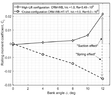
Figure 9. Cruise vs high-lift CRM configurations: opposite trends in the rolling moment coefficient vs bank angle at $\alpha = {8.0^ \circ }$ .

To illustrate the loss of the normal force coefficient throughout the span of the wing a spanwise normal force distribution is shown in Fig. 10. The solid lines demonstrate the spanwise distribution of the normal force coefficient for the cases with $\phi = {0^ \circ }$ and the dashed lines represent the cases with $\phi = {4^ \circ }$ and $\phi = {10^ \circ }$ . It is evident that the most significant loss of the normal force occurs on the right wing. And as mentioned earlier the wing tip having the longest arm generates a significant amount of the rolling moment, see Fig. 8.

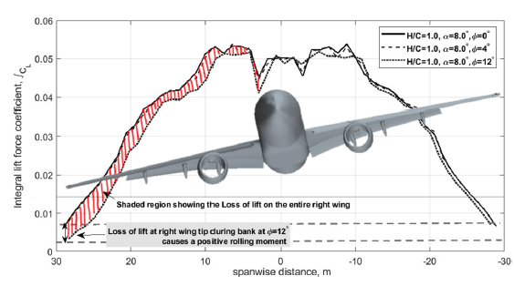
Figure 10. Accumulated lift force coefficient in spanwise direction at different bank angles in close-proximity to the ground at $h/c = 1.0$ and $\alpha = {8.0^ \circ }$ .

The loss of the normal force on the wing is related to the changes in the pressure on the wing surface. In order to compare the pressure coefficient distribution at a fixed location, the coefficient ${C_p}$ is plotted for a cross-section cutting the wing in the $x$ direction at $90{\rm{\% }}$ semi-span distance. The ${C_p}$ plots are shown in Fig. 11. Blue colour-filled circle markers show the ${C_p}$ for the case with zero-bank angle and the red colour-filled circles represent the ${C_p}$ values for the case with bank angle $\phi = {12.0^ \circ }$ .

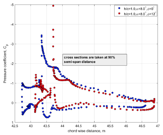
Figure 11. Pressure coefficient ${C_p}$ distributions at $90{\rm{\% }}$ semi-span distance for $\phi = {0^ \circ }$ and $\phi = {12.0^ \circ }$ in close-proximity to the ground at $h/c = 1.0$ and $\alpha = {8.0^ \circ }$ .

The most noticeable trend in this comparison is that the peak suction pressure on the main wing section is higher for the case with $\phi = {12.0^ \circ }$ than for the case with $\phi = {0^ \circ }$ . However, this is only true for a very small portion of the leading edge of the main aerofoil. It can be stated that when $\phi = {12.0^ \circ }$ , for the majority of the chordwise distance of the slats and the main wing section, lower positive pressure and also lower suction pressure are generated leading to an overall lower integral value of the normal force coefficient.

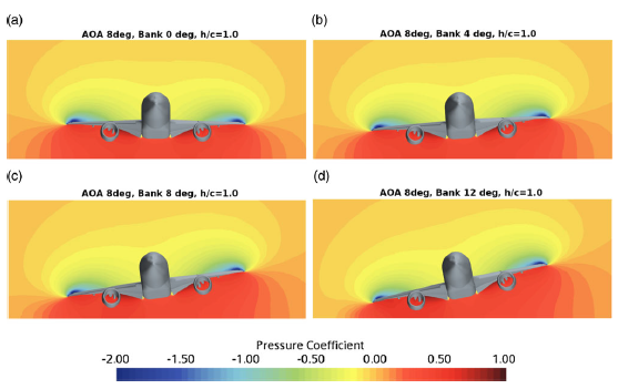
Figure 12. Flow field pressure coefficient ${C_p}$ contours in cross-section taken at $x = 37{\rm{m}}$ in different bank configurations at $\alpha = {8.0^ \circ }$ , $Re = 5.49 \times {10^6}$ , and $M = 0.2$ .

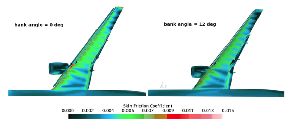
Figure 13. Skin friction coefficient ${C_f}$ contours on the upper surface of the wing for different bank angles at $\alpha = {8.0^ \circ }$ , $Re = 5.49 \times {10^6}$ , and $M = 0.2$ .

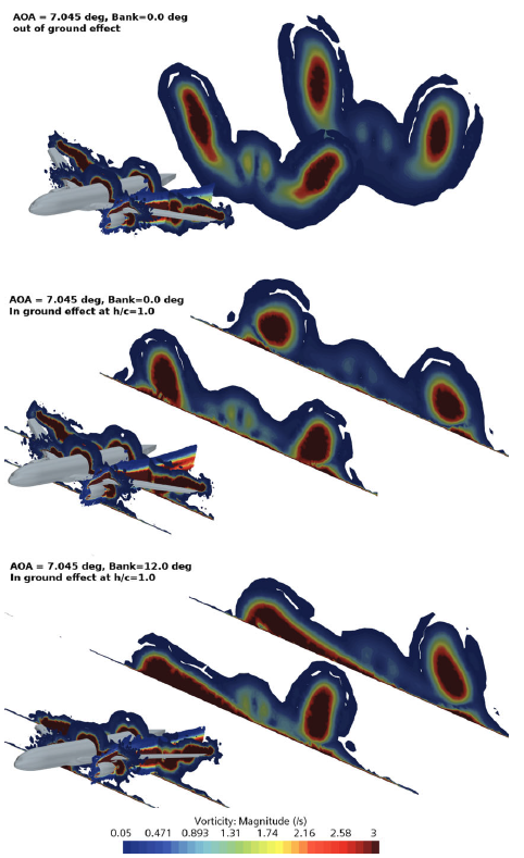
Figure 14. Flow field vorticity contours behind the CRM-WB-HL configuration in out-of-ground and in-ground effect at $\alpha = {7.045^ \circ }$ , $Re = 5.49 \times {10^6}$ , $M = 0.2$ , flaps inboard $/$ outboard $ = {40^ \circ }/{37^ \circ }$ .

4.3 Post-processing of the flow field in ground effect

The analysis of the flow field is carried out using the Star-CCM+ CFD post-processing tools. Figure 12 shows the pressure coefficient contours in a plane cross-section behind the centre of gravity at $x = 37{\rm{m}}$ at a height-to-chord ratio of $h/c = 1.0$ for four different bank angles $\phi = 0,4,8,{12^ \circ }$ . When $\phi = {0^ \circ }$ , as expected, a symmetrical pressure coefficient distribution is observed. With the increase in bank angle, the high-pressure zone on the right wing side of the aircraft model reduces. This effect is maximum when $\phi = {12.0^ \circ }$ , leading to the loss of the normal force coefficient as seen in Fig. 8.

In Fig. 13 the skin friction coefficient ${C_f}$ contours on the upper surface of the wing are shown at $h/c = 1.0$ and $\alpha = {8.0^ \circ }$ . The flow separation on the upper surface of the wing is more profound when $\phi = 12.0$ in comparison to the zero-bank position. More specifically there is a larger separation zone (see the black colour region in Fig. 13) towards the tip of the wing and also on the outboard flap, which also explains the loss of the normal force coefficient on the right wing (Fig. 8).

Further visualisations are carried out using vorticity contours projected on four distinct plane cross sections orthogonal to the fuselage of the aircraft in the x-direction and further behind downstream of the fuselage. These cross-sections are shown in Fig. 14. The changes in the vorticity and flow structure behind the wing are quite informative. When compared to the out-of-ground effect simulations, in close proximity to the ground at $h/c = 1.0$ the size of the two counter-rotating vortices which are shed behind the plane decreases in their radial circumference and maintains structure but does not get distorted. The influence of downwash is quite clear in this process. At $h/c = 1.0$ the vortex pair on the two sides are no longer identical and more interestingly, the vortex behind the right wing has broken down and deformed into a stretched but high-intensity vorticity zone. At this point, it is clear that the vortex formation and their topology during the ground effect phenomenon is certainly different from that of out-of-ground effect simulations, a deeper and detailed conclusion needs further investigation.