Introduction

The observations of microwave brightness temperatures of the Greenland and Antarctic ice sheets showed surprisingly low values and no clear relationship to the physical temperatures (Reference Gloersen, Gloersen, Wilheit, Chang, Nordberg and CampbellGloersen and others, 1974). Simple considerations of radiative transfer indicated that reflection at the snow-air interface was not sufficient to lower the emission to the observed values and therefore considerable radiative scattering must be occurring within the medium (Reference Gloersen, Gloersen, Wilheit, Chang, Nordberg and CampbellGloersen and others, 1974). The radiative transfer calculations by Reference Chang, Chang, Gloersen, Schmugge, Wilheit and ZwallyChang and others (1976) for a uniform snow medium showed that volume scattering by the snow crystals should be a dominant factor affecting the microwave emission. In order to make quantitative comparisons of observations and calculations it is necessary to account for the variations of snow properties with depth, such as the physical temperature and the crystal sizes. It is also necessary to define a general emissivity for bulk emitting media, because the usual definitions are not adequate for non-isothermal and non-homogeneous media.

In this paper, radiative transfer theory is formulated in terms of a radiative transfer function. An effective physical temperature is defined and used to define a general bulk emissivity. An approximate radiative transfer function, which is valid if the volume scattering is small relative to the absorption, is used to calculate the brightness temperature, effective physical temperature, and emissivity in order to illustrate the effects of various absorption and scattering coefficients and temperature variations. It is also used to calculate emissivities based on snow crystal size measurements for comparison with observed emissivities and to estimate the sensitivity of the emissivity to changes in the snow characteristics.

Emissivity and Brightness Temperature

The purpose of this section is to define emissivity ∊ and brightness temperature T _B consistently for snow and other bulk emitting media. The term brightness temperature, as an expression of the radiative intensity (radiance), is usually unambiguous. However, the meaning of the term emissivity is often ambiguous for a number of reasons. The emissivity is sometimes defined as the ratio of T _B to the physical temperature T (Equation (5)) and sometimes as the ratio of the radiance of a non-black body to that of a black body at the same temperature (Equation (2)). Also, it is sometimes interchanged with emittance, which is a microscopic property of the medium. And finally, of most importance to the consideration of emission from snow, the usual definitions of emissivity are only appropriate for isothermal media or for media that emit only from a thin isothermal surface layer.

The radiance or intensity (energy flux per unit wavelength per unit solid angle) emitted by a black body at wavelength λ is given by Planck's function

(1)

where b_λ = 2ck/λ⁴ and a — hc/λk (h, c, and k arc Planck's constant, velocity of light, and Boltzmann's constant respectively). Now, the emissivity e of an isothermal body that emits a radiance W(T), but is not necessarily a black body, can be readily defined as the ratio

(2)

The emissivity so defined may vary between o and i and it describes the relative ability of a body to emit energy.

In the Rayleigh-Jeans approximation for long wavelengths (a/T ≪ 1), Equation (1) becomes W_λ(T) = b_λT, which is the basis of the usual definition of T _B as

(3)

The brightness temperature is simply the emitted radiance expressed in units of temperature. Combining Equations (2)and (3) relates T _B to ∊,

(4)

and in the Rayleigh-Jeans approximation

(5)

which is applicable to isothermal media.

Although Equation (5) is sometimes used to define e, it is only consistent with Equation (2) in the long-wavelength approximation. Another quantity sometimes defined is the temperature, denoted as T _e, of the black body that produces a radiance equivalent to W_λ'(T). However, T_e is equal to T _B only in the same limit, i.e. setting T _B = W_λ(T_e) and using Equation (1) gives

(6)

Emissivity is a useful concept that describes the emissive characteristics of a medium. However, its definition for bulk emission from a non-isothermal medium must reflect the weighting of (he absorption, emittance, and scattering properties as they control the radiative transfer within the medium and, thus, control the externally observed emission. Ideally, emissivity would be independent of the temperature distribution T(z) in the body; but such a general definition is not possible, because among other reasons, some of the properties controlling the radiative transfer are also functions of temperature.

In order to define bulk emissivity, a radiative transfer function f(z) at wavelength A is first defined as the ratio of the increment ΔW_λ' of externally emitted radiation from the depth increment Δz to the radiation internally emitted at depth z in the medium, taken in the limit of small Δ.z,

(7)

where e(z) is the local emittance (dimensionless). Therefore, given ƒ(z) the radiance is

(8)

In effect, f(z) describes the transfer of radiation from point z to z = 0. Since the emission and absorption considered here are thermal, Kirchhofes law applies and, thus, the emittance is

(9)

where

(10)

and where the extinction coefficient γ_e(z), the absorption coefficient γ_a(z), and the scattering coefficient y_s(z) are in units of inverse length. Also, the scattering albedo ω₀ is

(11)

The quantity [f(z)e(z)] in Equation (8) is similar to the weighting function F(z) used to calculate the microwave radiative transfer in the earth's atmosphere, i.e.

In general, to consider the radiance in direction (θ,φ), the function f(z) is replaced by f(z, θ, φ) and z by z sec θ

An effective black-body radiance is defined here using ƒ(z),

(12)

and an effective physical temperature is defined as

(13)

Physically, the effective physical temperature is an average physical temperature weighted by the radiative transfer properties, which are described by ƒ(z). The bulk emissivity can now be defined similarly to Equation (2),

(14)

This emissivity also has (he property of varying between 0 and 1, since the emittance e(z) can only have values between 0 and 1 and f(z) and W_λ(z) in Equations (8) and (12) are positive definite. In physical terms, the bulk emissivity is the ratio of the emitted radiance to the radiance from a hypothetical medium having the same radiative transfer function but having each volume element of the medium emit as a black-body. It should be noted that f(z), Ye(z), Ya,(z), Ys(z), w₀(z), e(z), and ∊ are implicitly dependent on wavelength λ. In the Rayleigh-Jeans approximation, the bulk emissivity is the ratio of the brightness temperature to the effective physical temperature,

(15)

which is similar to Equation (5). However, the bulk emissivity is not directly measurable because 〈W_λ 〉 (or (T)) is not directly measurable, in contrast to W_λ (or 〈 T〉) in the isothermal case. Nevertheless, W_λ (or (T)) can be estimated or measured for certain cases as will be shown later.

Several important properties of the bulk emissivity may be noted using Equations (8), (12), (13), and (14). First, if the medium is isothermal, then 〈W_λ 〉 = FW_λ where

(16)

and the emissivity is

(17)

Note that Equation (17) differs from the usual definition for isothermal media (Equation (2)) if F ≠ 1,as will be discussed later for optically thin media. Second, if the emittance is not a function of depth (that is, if e is constant) even though the medium is not isothermal, then the bulk emissivity equals the emittance (∊ = e), independently of the temperature distribution. Therefore, the second property shows that it is the variation of emittance with depth that makes the bulk emissivity dependent on T(z), and equivalently that the bulk emissivity of a homogeneous medium is independent of T(z).

Radiative Transfer Problem

The radiative transfer function ƒ(z) for a given medium is physically determined by the absorption, emittance, and scattering properties of the medium and it contains all the information required to calculate the emitted radiance. In effect, ƒ(z) describes the efficiency for external emission of radiation from a source at point z or, as previously noted, the transfer of radiation from point z to z = 0. For example, consider the case of pure absorption for which γ_e = γ_a and e = 1. Then,

(18)

In this pure absorption case, the radiative transfer function is

(19)

and the bulk emissivity is unity as it should be for a pure absorber. Thus, (he transfer function in this case decreases exponentially with depth.

In general, a solution of the radiative transfer equation is required to determine ƒ(z) To show how the radiative transfer function ƒ(z) is determined, it is first noted that ƒ(z) is in fact similar to the source function used in astrophysical radiative transfer problems and to the function for the probability of quantum exit formulated by Reference SobolevSobolev (1956, chapter 6). The radiative transfer equation (Reference Chang, Chang, Gloersen, Schmugge, Wilheit and ZwallyChang and others, 1976; Reference SobolevSobolev, 1956), may be written as

(20)

where the source function is

(21)

and F_λ(z, θ, φ, θ_s, θ_s) is the scattering phase function and dw_s is the differential solid angle. The integral equation form of Equation (20) for the radiance at z = 0 is the well-known formula (Reference SobolevSobolev, 1956, English translation, p. 17 and 30; Reference AllerAller, 1963, p. 217)

(22)

where τ(z) is the optical depth,

(23)

Comparing the generalized form of Equation (8) ƒ(z) → ƒ(z, ,θ,φ) and z →z sec θ) with Equation (22), shows that the relation between the radiative transfer function and the source function is

(24)

Therefore, given γa(z), Ye(z), T(z), and F_λ(z, θ, φ, Θ_s, φ_s) the radiative transfer function can be calculated.

For isotropic scattering, the integral in Equation (21) can be replaced by 4πJ_λ(z), where Jλ(z) is the mean radiance averaged over all angles, so that

(25)

and, hence,

(26)

In this case, the source of the radiation is the sum of the isotropically scattered radiation and the isotropic emission. If the scattering is small relative to the absorption and emission (ω₀ ≪ e), then f(z, Θ) may be approximated by

(27)

In the next section, g(z) is used to illustrate the effects that the vertical gradients of T and y_s have on the emission. Using g(z) instead of ƒ(z) is equivalent to neglecting the scattered radiation in the source term. Neglecting a source term reduces the emitted radiation and consequently, the g(z) approximation should tend to over-estimate the effects of scattering.

Model Calculations

The coefficients γa(Z) and γs(Z) provide information on the emissive properties of the medium even if the radiative transfer equation is not solved exactly. Given γs(Z), Ya(Z), and T(z), the brightness temperature, effective physical temperature, and the bulk emissivity can also be approximated using g(z),

(28)

(29)

and the emissivity by Equation (15). The Rayleigh-Jeans approximation has been taken here for convenience. The Equation (28) shows that, in this approximation, the relative contribution to the external radiance from the emission at depth z is simply the emission per unit length times the damping of the overlying material given by exp [— τ(Z)]- The calculations in this section using g(z) show that g (z) is very useful for approximately describing the emissive properlies of a snow medium. The Equations (28) and (29) arc solved here using a γa which is independent of depth and a y_s which increases linearly with depth. Therefore,

(30)

It is shown below that these coefficients are realistic for polar firn except for large z.

Table I. Mie scattering and absorption coefficients for. N_r = (2r)^-3 and λ = 1.5 cm

Table I lists some Mie scattering and absorption coefficients (Reference Chang, Chang, Gloersen, Schmugge, Wilheit and ZwallyChang and others, 1976) for wave length λ = 1.5 cm and for different values of the ice-particle radius r and imaginary part n” of the index of refraction. The y_s is essentially independent of n”. The values of n” = 0.002 4 and 0.000 55 correspond to solid ice at 0°C and —20°C respectively as measured at λ = 3.2 cm (Reference Cummingcumming, 1952). There is, however, a considerable discrepancy in the published values of the loss tangent (reviews by Reference EvansEvans (1965) and Rover (1973)). The loss tangent is

(31)

where n’ is the real part of the index of refraction. In addition, n” may be greater at the λ= 1.5 cm used here than it is at 3.2 cm. Nevertheless, the higher absorption value (n” = 0,002 4) is taken here to be indicative of warm ice near the melting point and the lower values to be indicative of cold ice. The coefficients in Table I are the Mie cross-sections multiplied by the density N _r of scatters, which was taken to be N _r = (2r)^-3 and corresponds to a snow density of 480 kg/m³. It is also noted that the absorption of solid ice,

(32)

is approximately equal to the y_a values listed for r = 5 mm and about three times the y_a values for the smaller r.

The Mie absorption coefficients in Table I are nearly independent of r for r ≲, 0.5 mm. The scattering coefficients can be approximated within a few percent for r ≲ 1 mm by y_s = (1.8r)³. The r³ dependence arises for the following reasons: for r small relative to λ, the Mie scattering cross-section σ_s varies as r⁶ (Rayleigh scattering region) and y_s equals N _rσ_s, which is then proportional to r³. To obtain the dependence of r³ on z, crystal-size data measured at seven locations in Greenland and Antarctica arc used (see Table II). The analysis by Reference GowGow (1969, 1971) indicates that the crystal growth depends on time / and temperature T according to

(33)

where k is a constant, E is the activation energy of the growth process, and R is the gas constant. Using t = σ(z)/∊ (i.e. snow load divided by mean accumulation rate) and taking σ(Z) = ρ₀z+ριZ² would give a quadratic dependence of r² on z. Gow's analysis shows that Equation (33) fits the data well below 10 m if T _m is taken to be the mean annual temperature T _m, but not as well above 10 m. The effect of the time variation of T above 10 m is to cause a higher average growth rate nearer to the surface; thus, the curves of r² versus t or z might be expected to have a negative curvature above 10 m and such negative curvature is exhibited by the data. In fact, a regression analysis for

(34)

gives a good fit to the crystal size data over the depth region from which most of the microwave radiation emanates (i.e. ≲ 30 m) and a better fit above 10 m. The resulting regression coefficients for Equation (34) are listed in Table II. Although functions other than Equation (34) might be used for representing the data, the chosen function also gives the desired linear dependence for the scattering coefficient in agreement with Equation (30).

Table II. Crystal size profiles and scattering coefficients using r³ = r ₀ ³ +az regression fit

In order to use the linear function for y_e given by Equation (30), it is necessary to neglect the increase in snow density with depth and neglect the dependence of the n” on temperature. Then, Equation (30) can be used as a good first-order approximation to γe(z) for r ≲ 1 mm and for, . It accounts for a most important variable, that is the variation of crystal sizes and scattering with depth.

Using Equation (30) to solve Equations (28) and (29), first for the case of constant T, illustrates the dependence of the emissivity on the relative values of the scattering and absorption coefficients. Taking the medium to be optically thick (that is exp [—_T(∞)] = 0) and using

(35)

gives 〈T〉 = T. Equation (28) is solved first by setting γ_{s o} = O and the resulting emissivity is

(36)

where x =y_a/(2S)^½ and φ(x) is the error function. The emissivity obtained by Equation (36) for various values of the absorption and the scattering coefficients is shown in Figure 1. Although it is known from consideration of the scattering albedo alone that scattering is more effective at the lower absorption values, Figure 1 illustrates the high sensitivity to scattering if the absorption is low. As y_a changes by an order of magnitude, the scattering term, y_s, must change by about two orders of magnitude to give the same emissivity. This is due to the respective dependency of ∊(x) on y_a and s^½ .

Fig. 1. Emissivity as a function of the linear scattering coefficient for various absorption coefficients using g(z) and constant T.

The constant term (γ_s)_o) in y_s according to Equation (30) can also be simply accounted for by solving

(37)

where y_a' = y_a+y_{s o}) and x' = γ_a /(2S)^½. The effect of y_{s o} is to reduce the emissivity. For example, taking y_a = 0.2 and neglecting y_{s( o}, gives ∊ = 0.51, whereas including y_{s o} gives a lower value of ∊ = 0.37 due to greater scattering.

In the next section, emissivities are calculated for the locations listed in Table II. It should be noted that, for the y_a and y_s values in Tables I and II, the approximation ω₀ $$ e required for the use of g(z) is not really valid. However, the results below using g(z) should be al least qualitatively correct. Also, the results in a later section comparing calculated and observed emissivities, imply that the y_s is not as large as the values in Table II.

Fig. 2. High absorption case showing (g(z)e(z)) and g(z)for various linear scattering coefficients.

Figure 2 illustrates the weighting functions (g(z)e(z)) and g(z) used to calculate T and 〈T〉 respectively for a case of high absorption (y_a = 0.5/m) and different depth-gradients of the scattering coefficient [γ_s = sz). The γ_so is set equal to zero. The radiation from a depth increment Δz is and, as the scattering increases, the emitted radiation becomes more restricted to the near-surface material as shown in Figure 2(a). In the case of low absorption (y_a = 0.1/m), the radiation emanates from a greater range of depths as shown in Figure 3(a) and a layer of given optical thickness must be about five times as deep in contrast with the high absorption case. The contribution to the emission from depth z is g(z)e(z) = γ_a (Z) exp [— r(Z)]. However, it must be remembered that g(z) is a small-scattering approximation ƒ(z) that is quantitatively valid only for y_a y_a.

The g(z) curves in Figures 2(b) and 3(b) illustrate the effectiveness of the various depths for a hypothetical medium having the same radiative transfer function as the real medium, but having a black-body emittance e(z) = 1. Using Equations (10) and (27) in Equation (29) shows that 〈T〉 is equal to T _B plus a term , which depends on the scattering coefficient. Thus, the hypothetical medium has an emission per unit length determined by y_e = γ_a+γ_s. For the larger s values, g(z) peaks at z > 0 because y_s(Z) is increasing faster for small z than exp [—_T(Z)] decreases. Using Equation (35) it is also noted that, for an optically thick medium, the area under the g(z) curve is unity; thus, as some layers become more effective due to changes in y_s, other layers must become less effective in weighting the physical temperature.

Fig. 3. Low absorption case showing (g(z)e(z)) and g(z) for various scanning coefficients.

An additional property of the bulk emissivity can be conveniently noted at this point. Consider the emission from a medium of thickness z_m that is not optically thick. The brightness temperature then strongly depends on the thickness z_m and Equation (5) is meaningless. However, the effective physical temperature also depends on _Zm in a similar manner, so that the bulk emissivity does not strongly depend on z_m unless e(z) also varies strongly with z. For example, in the case of constant T

(38)

which is always less than or equal to T because G $$ 1, and the bulk emissivity is

(39)

Therefore, the bulk emissivity of an optically thin medium is indicative of the emissive properties, in contrast to T_B, which depends strongly on the thickness. As noted before, G = 1 for an optically thick medium.

It would be useful to consider a descriptive parameter z’ as the depth above which a fraction β' of the radiation emanates,

(40)

Since Equation (40) requires solution of the radiative transfer equation, a more simple parameter ß is defined,

(41)

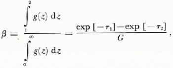
which may be viewed as the approximate relative effectiveness of the layer z₂ — z₁. For Z₁ = 0 and an optically thick medium,

(42)

which will be calculated for some characteristic polar firn properties in the next section.

To examine the seasonal properties of T _B and (T), a time-dependent temperature profile illustrated in Figure 4 is chosen,

(43)

Fig. 4. Model temperature profiles at various times relative to time of surf ace temperature maximum.

Fig. 5. (a) High absorption case, (b) low absorption case; effective physical température (T) and brightness temperature T_B, for two values of the linear scattering coefficient, and the surface temperature T_s as a function of time.

where the mean surface temperature is T_m = 250 K, the amplitude (2A) at the surface is ₃₀ K, the surface temperature (T_s) is a maximum at t = o d, and the other coefficients are appropriate for the firn at Maudheim (lat. 71° 03'S., long. 10° 56' W.) (Reference Dalrymple, Dalrymple, Lettau, Wollaston and RubinDalrymple and others, 1966, p. 42). The Equations (28) and (29) for T _B and 〈T〉 are numerically integrated for the high absorption case (Figure 5a) and the low absorption case (Figure 5b), and for high and low scattering in each case. A number of characteristics are illustrated by these curves. First, the amplitudes of the seasonal variation of both T _B and 〈T〉 are larger in the high absorption case, because for high absorption the near-surface material (where the T variation is large) is more effective in emitting whereas the material below 6 m has smaller weighting; in the low absorption case there is significant weighting of levels below 10 m (where the T variation is small). In contrast to the change in amplitude due to a change in absorption, the change in amplitude due to a change in scattering is not as marked, which is a feature that can also be discerned from the relative weighting functions and the temperature profiles in Figures 2-4. Second, a phase lag is evident in the seasonal variation of T _B and 〈T〉 relative to the surface temperature variation. The phase lag is about 20 d in the high absorption case and about 40 d in the low absorption case; the difference in these phase lags is also due to the greater weighting in the low absorption case of the deeper z levels where the temperature phase lag is larger. As with the amplitude characteristics, the difference in the phase lags due to high as opposed to low scattering is not as marked as the difference due to high as opposed to low absorption. These features can also be discerned from the respective weighting functions in Figures 2 and 3. Finally, although T _B decreases markedly with increased scattering! (T) changes by less than several kelvins; increased scattering makes 〈T〉 slightly warmer in summer and slightly cooler in winter because the emission is more limited to the material nearer the surface.

Fig. 6. (a) High absorption case, (b) low absorption case; bulk emisswity ∊ and approximate emissvity E, for two values of the linear scattering coefficient, as a function of lime

Figures 6(a) and (b) illustrate the emissivities according to Equation (15) for high and low absorption. The emissivity ∊ varies slightly with time because T _B is weighted slightly more at the shallower z than 〈T〉 is; this effect increases with increased scattering. Also shown is an approximate emissivity, determined by the surface temperature,

(44)

which will be considered in a later discussion on observations. The curves of E, in contrast to those of ∊, show that T_s is not a very good measure of the physical temperature for estimating the emissivity, unless g(z) is concentrated at shallow z due to high absorption and/or high scattering.

Calculated and Observed Emissivities

The periodic nature of the temperature and emissivity variations as shown in Figures 5 and 6 suggests a means for measuring the bulk emissivity, even though (T) is not directly measurable. Since the surface temperature (T) _s intersects (T) twice each cycle, ∊ equals £at the cross-over times, which are between 60 and 80 d after the extrema in T _s for the given examples. However, this method is limited because the cross-over time is not known a priori and T_s must be averaged over short-term fluctuations. Nevertheless, E measured at about t = 2.5 or 8.5 months would approximate ∊. An accurate average ∊ can be obtained, however, by averaging both the physical surface temperature and T _B over a one-year cycle. Using Equation (43) or a similar periodic function in Equation (13) and averaging over one cycle gives

(45)

where T_m is the mean annual surface temperature. The mean bulk emissivity is then

(46)

where T_B is the mean annual brightness temperature. If the medium is optically thick, then F should equal unity and Equation (46) becomes the ratio of physical observables. In general, however, ƒ(z) is also time dependent and the time dependence of T(z, t) may be such that Equation (45) might not be exact.

The mean emissivity is a physically measurable quantity which can be used to compare theory and observations of optically thick media. The calculated emissivities using the y_s given in Table II, which are based on the crystal-size data from seven locations, are shown in the first column of Table III. The mean annual _TB has been obtained by averaging twelve monthly observations by the Nimbus-5 ESMR (Reference Wilheit and SabatiniWilheit, 1972) between September 1973 and August 1974. Each monthly observation is typically the average of 15 measurements from overlapping scans during periods of three days each. A scan-angle-dependent correction (Reference WilheitWilheit, 1973) has been applied to the horizontally polarized ESMR measurements which reduces the limb darkening caused by variation of the scan angle, so that each measurement approximates a nadir observation normal to the surface. The averaging of measurements from differing scan angles further reduces the limb-darkening uncertainty. The resulting are used to calculate the observed emissivities ∊_OBS shown in Table III. Also, listed in Table III are some E values which are less than ∊_OBS because summer T _s values are used. Although the ∊_OBS values are about twice as large as the calculated values ∊_CALC in the first column of Table III, the predicted negative correlation between ∊_OBS and y _s can be seen by comparing locations with similar y_so (for example South Pole and “Plateau” or Camp Century and Inge Lehmann).

Table III. Calculated and observed emissivities

The probable causes of the discrepancy between ∊_CALC and ∊_OBS are: (1) overestimation of γ_s by the scattering model which assumes each snow crystal to be an independent scatterer despite the fact that the crystals are packed within a few diameters of each other and (2) overestimation of the scattering effect by using the approximate radiative transfer function g(z) instead ƒ(z). Secondary causes are: (3) uncertainty in y_a due to the scattering model and the uncertainty in the measurements of n”, (4) neglect of the dependence of n” on T(z), and (5) neglect of the snow density variation with depth.

Under the hypothesis that the ∊_CALC overestimates the scattering effect, the scattering coefficient is multiplied by an empirical parameter to obtain agreement with ∊_OBS For γ_a = 0.15, good agreement is obtained by using y._s' = o. 12y_s. This smaller y_s', in contrast to y_s, makes the g(z) approximation more valid. Similar agreement can also be obtained for other y_a values as shown in Table III, but the slope of ∊_CALC versus ∊_OBS changes due to the differing effect of the scattering as absorption changes. Figure 7 shows the relationship between ∊_CALC and ∊_OBS for y_a = 0.15 and y_s' = 0. 12y_s. The agreement for the five locations where crystal sizes were measured by the same investigator (Gow) is good. In addition, for these five points the increasing relative difference between ∊_CALC and ∊_OBS as the emissivity decreases is consistent with the increasing error expected due to the g(z) approximation as the scattering increases and emissivity decreases, but the other factors such as the dependence of n” on T must also be considered. The dependence of n” on T below —20°C at about 20 GHz is small, but is difficult to estimate from available data (Reference RoyerRoyer, 1973). However, it appears to be no more than 20% smaller for the temperatures typical of the colder firn at South Pole and “Plateau”, in comparison to the other stations. Making n” smaller by 20% would reduce ∊_CALC by 4.8% for South Pole and by 6.6% for “Plateau”, but would not change the basic agreement shown in Figure 7.

Fig. 7. Calculated mean bulk emissivities versus observed values at seven locations (see Table III). Scattering coefficient is determined by crystal-size measurements and an empirical parameter equal to 0. 12. Solid circles (•) indicate crystal measurements by Gow, open circles (○) indicate measurements by other investigators, and crosses(X)indicate a 20% adjustment was made to crystal sizes measured by other investigators.

The discrepancy between ∊_CALC and ∊_OBS for Site 2 and “South Ice” as shown in Figure 7 may be due to a difference in the crystal-size measuring techniques as discussed by Reference GowGow (1969). Since thin-section analysis seldom cuts crystals at their maximum diameter, Gow notes that Reference KrumbeinKrumbein (1935) found that the most frequent radii are only about 80% of the true diameter. Gow, in contrast to the other investigators, attempted to remove this bias by selecting the 50 largest crystals (typically 25% of the total crystals) in each section. Therefore, the crystal sizes at “South Ice” and Site 2 arc likely to be about 20% too small relative to Gow's values due to this bias. Increasing the crystal radii listed in Table II for Site 2 and “South Ice” by 20% and recalculating ∊_CALC gives good agreement with ∊_OBS for these two locations also, as indicated in the figure.

On the basis of the agreement exhibited in Figure 7 it is concluded that the calculations using g(z) and one empirical parameter provide a simple semi-empirical model for calculating the effects of changing accumulation rate, changing mean annual temperature, or the effects of the other variations in snow properties that have been neglected. The model is not capable of indicating which are the best choices of both y_a and y_s. Nor is it capable of indicating whether the Mie/Rayleigh scattering model really does over-estimate the scattering coefficient by a factor of the order of 5 to 10. Nevertheless, the results do support the previous conclusion (Reference Chang, Chang, Gloersen, Schmugge, Wilheit and ZwallyChang and others, 1976) that the crystal or grain size is the primary parameter determining the microwave emissivity of dry polar firn. This relationship is also illustrated by comparing the observed emissivities directly with the measured crystal-size gradients as given in Table II, without regard to any model. The significance of this dependence of emissivity on the crystal-size gradient will be discussed in the next section on accumulation rate.

Fig. 8. Functions (g(z)e(z)) and g(z) using empirically adjusted scattering coefficients for South Pole and “Byrd” locations,

Table IV. Depths in meters for different optical depths, the aver ace depth (Z), and at one optical depth

Using the empirically adjusted scattering coefficient significantly increases the range of depths from which radiation is observed. Figure 8 illustrates the radiative transfer function and (g(z)e(z)) for the South Pole and “Byrd” locations. The differing emissivities of these two locations is caused by a relatively small difference in the illustrated functions extending over the range of effective depths. The parameter β given by Equation (42) is used to illustrate the approximate effectiveness of a particular depth range. Table IV lists the depths corresponding to given optical depths and β values. An appropriate β to consider is β = 0.993 corresponding to five optical depths and all but 1 to 2 K of a typical T_B value. Thus, the values in Table IV indicate that it is necessary to consider the firn radiation from a depth of at least 30 m. However, the accuracy to which the snow properties must be known decreases approximately exponentially with depth. Another descriptive parameter, the average depth, is defined,

(47)

The values of (z) using. g(z) are listed in Table IV along with the firn age at one optical depth from data given by Reference GowGow (1969, 1971).

The discrepancy between ∊_CALC and ∊_OBS due to the g(z) approximation can be reduced by numerical solution of the radiative transfer equation layer by layer (e.g. Reference Chang, Chang, Gloersen, Schmugge, Wilheit and ZwallyChang and others, 1976). The empirical parameter in y_s' should then mainly represent the discrepancy due to the independent snow-crystal scattering model. Then, the slope and the magnitude of ∊_CALC versus ∊_OBS should together provide information on the appropriate values of both γ_∊ and y_s.

Accumulation Rate and Emissivity Sensitivity

The model of the previous section, which uses an empirical parameter in the scattering coefficient, permits the calculation of the emissivity change resulting from a change in the accumulation rate A. Since Equations (33) and (34) do not give the same relationship between r and z, as noted previously, the functional relationship between a and A is not clear, but can be approximated as inverse linear. The substitution

(48)

may then be used to obtain the emissivity as a function of K or A, where K = A_o/A and A_o is the measured accumulation rate. The results using γ_∊ = 0.15 and y_s' = 0.12y_s are shown in Figure 9. The limit in each case as K-> o is γ_∊ γ_a', which is the limit of zero crystal growth rate or infinite accumulation rate. The conditions at South Pole arc not far from this limit, because the growth rate is small due to the cold temperature and the accumulation rate is relatively high for a cold region. Also indicated in Figure 9 is the direction each curve would shift for different A or T_m; the relative displacement of a pair of curves having similar T _m is about the same as their A_o ratio. From these curves, the change in emissivity resulting from a change in average accumulation rate can be estimated at each location. The sensitivities (∊_o,Δε∊Δ∊) calculated at K — 1 are listed in the figure. At Camp Century, for example, a 10% change in accumulation would change the emissivity by 0.01, A change of this magnitude corresponds to a T_B change of 2 K, which is of order of the radiometer measurement accuracy. At South Pole where the crystal-size gradient is small, the sensitivity is a factor of five smaller. The sensitivity is lowest in colder regions of higher accumulation, and highest in warmer regions of low accumulation such as north-east Greenland. Returning to Figure 7, where the arrows indicate the change of emissivity due to increasing A or T_m, it is also noted that the range of observed emissivities is narrowed by the tendency of colder locations to have low A, and of warmer locations to have high A.

Fig. 9. Emissivity as a function of K, which is approximately determined by the accumulation rate A_o or mean annual temperature T_m (see text).

Since it is the dependence of the emission on the gradient of the crystal size that causes the emission to depend on accumulation rate, it is essential for the observed radiation to emanate from a range of depths sufficient to cause a detectable sensitivity to the gradient. If the depth-gradient is small, it may be possible to obtain a greater sensitivity to accumulation rate by choosing a longer wavelength, for which y_s is less and the effective depth is thus greater. However, the increase in effective depth that can be so obtained is limited because the empirically adjusted y_s is so small that the effective depth is mainly determined by γ_a (see Fig. 3), and y_a does not vary strongly with λ. In fact, it seems fortuitous that the important parameters involved have the appropriate values to produce a measurable sensitivity to the accumulation rate at most locations of dry polar firn.

Since the microwave emission depends on an average accumulation rate over some years, a sudden change in the annual accumulation rate would only gradually change the emission. A parameter which approximates the time constant for such a change in emission is the age at one optical depth as listed in Table IV. Since the optical depths are approximately the same for all these stations, the time constant depends mainly on A and varies widely with location from about 7 years at Camp Century to 75 years at “Plateau”.

The other primary parameter affecting the crystal size and the microwave emission is the mean annual temperature. The sensitivity of the emissivity to changes in mean annual temperature can be estimated in a similar manner to accumulation changes. A relationship similar to that implied by Equation (48) is assumed so that

(49)

where T_mo is the measured mean annual temperature. The calculated sensitivities (Δ ∊ / ΔT) are listed in Table V. For Site 2 and “South lce” the crystal radii were increased by 20% (see previous section) before calculating the sensitivities. Referring also to the sensitivity to accumulation (Δ∊A_oΔA), it can be seen that a one degree change or uncertainty in T_m is approximately equivalent to a 10% change or uncertainty in A.

Comparison of Site 2 and Camp Century, which have essentially the same T_m, shows that the smaller crystal sizes measured at Site 2 and the higher observed emissivity arc consistent, and together indicate a higher A at Site 2. Using the difference in observed emissivities Reference MockMock, 1968, p. 16) indicates an A difference that ranges from 9% to 45% depending on the (Δ∊ = 0.045) and the estimated sensitivity (Δ∊A_o/Δ∊ = 0.098) indicates that A is 46% greater at Site 2. Using A values from surface measurements (Reference LangwayLangway, 1967, p. 94-95; measurements used; Mock's Camp Century value of 3i8kg/m² from 1955-62 firn stratigraphy and Langway's Site a value of 423 kg/m² from 1954-57 firn stratigraphy indicate a 33% difference. Such comparison is complicated by the different accumulation years represented by the various measurements, and the microwave observations, and also by significant accumulation gradients (Reference MockMock, 1968) over the surface within a resolution element of the microwave observations. Nevertheless, the accumulation value measured at the surface at Site 2 and that which is estimated from the observed emissivity agree well within the uncertainties of the methods.

Table V. Estimated emissivity sensitivities

Conclusions

The formulation of the radiative transfer problem using the radiative transfer function f(z) provides a useful general definition of emissivity of bulk emitting media. The g(z) approximation enables simple calculations of emissivity that account for the variations of snow properties with depth and illustrate the effectiveness of the various depths.

Although 5 m of typical firn corresponds to one optical depth at λ = ι. 55 cm, significant radiation emanates from depths up to 30 m or more. Consequently, the observed radiation is determined by firn layers deposited over many seasons and the effect of summer to winter differences in deposited snow crystal sizes should be minimal.

The bulk emissivity is relatively independent of the seasonal temperature variation, in contrast to the approximate emissivity determined by the surface temperature. The seasonal variation in the calculated T_B is shown to lag the variation in T_s Further analysis of the observed 7∊ over a year can be expected to provide additional information on the snow-emission properties.

An appropriate quantity for comparing calculations and observations is the mean emissivity (T_B/T_m). The agreement between the observed emissivities at seven locations and the calculated emissivities using one empirical parameter shows that the crystal-size variation with depth is a primary parameter influencing the microwave emission of dry polar firn. Since the crystal sizes are primarily dependent on A and T_m , these two quantities are measurable by microwave sensors, but not independently measurable with one microwave frequency. The estimated sensitivities of the emissivity are such that, given an independent T_m to an accuracy of 1 K and a radiometer accuracy of 1 K, the accumulation rate should be measurable to an accuracy of the order of 20% at most locations. The importance of a satellite measurement of accumulation will be in the capability to interpolate or extrapolate spatial patterns relative to locations of accurate surface measurements. Knowing the estimated sensitivities of emissivity to A and T_m it is now possible to interpret observed emissivity patterns of the ice sheets in terms of variations or anomalies in A or T_m. However, development of a more quantitative technique requires, in particular, additional measurements of crystal-size profiles and further study of the factors affecting the crystal-growth rates and initial sizes, as well as better measurements of the complex index of refraction as a function of wavelength and ice temperature.

Acknowledgements

I appreciate the assistance of Ms Dorothy K. Hall in analyzing brightness-temperature data. Also, the thorough review of the concepts in this paper by Mr Jack Saba were most helpful.