Gravity measurements

All gravity measurements were made with Worden gravimeter 236 (surveying model) belonging to the Division of Geological Sciences, California Institute of Technology. The dial constant of the meter given by the manufacturer is 0.1901 (5) mgal./small dial scale division, a value which agrees well when compared with a calibration range of several hundred milligals. Long-period meter drift averaged about 1 mgal./day. Earth tides and temperature changes caused greater short-period drift rates; however, drill of the instrument in the field did not exceed 0.2 mgal./hr. Drift corrections were distributed linearly with respect to time of observation.

Gravity was measured along 10 traverses transverse to the glacier (Fig. 1). The west end of each traverse was re-occupied to correct for meter drift and these stations were all tied together through a common base station. The meter does not have a range adequate to allow simple tying of the network to a known gravity value, so that only relative differences were obtained. These relative differences probably have errors of about 0.1 mgal.

Fig. 1. Bouguer anomaly map of lower Blue Glacier

Gravity stations

The seven northernmost traverses and the next to southernmost traverse were measured during August 1960 On the basis of the promise of these results two additional traverses were made in August 1961. A total of 146 stations was occupied, 20 of which are on bedrock. Elevations and positions of the stations at the ends of the traverses and of all the stations measured in the second year were determined by theodolite measurements from the triangulation network previously established by Meier around Blue Glacier (from a paper on surface-velocity and surface strain-rate data from lower Blue Glacier to be published by M. F. Meier, C. R. Allen, W. B. Kamb and R. P. Sharp). Small vertical refraction and curvature corrections to the vertical angle measurements were made using an empirical formula which gives good agreement on lower Blue Glacier for shots to the same point from different triangulation points. Station elevations the first year were determined by levelling on the glacier. Closure of the Ievel lines was less than 0.2 m. and this error was distributed evenly among the stations of the traverse. The elevations of the stations are probably known to the closest 0.2 m., which can produce in the Bouguer anomalies a possible error of 0.04 mgal. In addition it should be mentioned that station elevations were determined within 8 hr. of the gravity observations, so that ablation and down-slope movement of the glacier contribute little to elevation errors.

Bedrock and ice densities

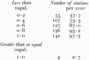
The density of the glacier ice was not measured but is assumed to be 0.9 g./cm.³ (Reference SeligmanSeligman, 1950). Low-grade metamorphic rocks of either Mesozoic or early Tertiary age form the bedrock surrounding Blue Glacier. The mean density of 33 relatively unweathered samples of bedrock collected at random from morainal deposits was determined by means of a, Jolly balance to be 2.73 g./cm.³ with a range from 2.68 to 2.77 g./cm.³. The variation in the measurements is shown in Table I.

Table I Bedrock Densities

Terrain corrections

The gravitational effect of the topography around each station was calculated by means of graticules using the scheme of Reference HammerHammer (1939) out to a distance of 6.7 km. from each station (through zone “J”). In areas of high relief an extension of the original tables (Reference CorbatóCorbató, 1963, p. 18–19) was utilized. Because of the availability of topographic maps of good quality (U.S. Geological Survey, Mount Olympus quadrangle, 1956, 1:62,500; American Geographical Society, 1960, Blue Glacier map, 1:10,000), it is felt that accurate terrain corrections can be applied to the data even though the magnitude of the corrections is high (from 6 to 13 mgal.). (The elevations of the glacier shown in the illustrations are based on the triangulation network of M. F. Meier, C. R. Allen, W. B. Kamb and R. P. Sharp for lower Blue Glacier. Comparison with the map of the American Geographical Society (1960) indicates a systematic difference between the two with Meier’s network having elevation values 9 m. below those of the published map. This error does not appear to be significant in computing the terrain correction.) The density used in making the corrections for all compartments is 2.73 g./cm.³. Reference KanasewichKanasewich (1963, p. 618) used the density of ice for compartments which are on the glacier but this implies a previous knowledge of the glacier configuration. It seems preferable to place this aspect of the problem into the interpretation of the anomalies. Figure 2 shows the surface elevations during the summers of 1960–61 and the approximate configuration of the terrain correction function. The divergence of this function from a simple form indicates that simplifying assumptions (e.g. Reference Bull and HardyBull and Hardy, 1956) can introduce large errors. Repeated computation of terrain corrections on Blue Glacier indicates that these values have a precision of about 0.1 mgal. and an accuracy of perhaps ±0.2 mgal.

Fig. 2. Surface elevations (1960–61) and terrain corrections

Elevation and latitude corrections

An elevation correction (combined free-air and Bouguer) was computed for each of the stations using a factor of 0.1943 mgal./m., corresponding to a density of 2.73 g./cm.³. In addition latitude corrections were calculated using the standard international gravity formula.

Bouguer anomalies

The Bouguer anomalies (Fig. 1) represent the observed gravity values corrected for topography, elevation and latitude. The datum is an arbitrary one as only relative differences in gravity were observed. One would expect these anomalies to reflect basically the mass deficiency of the glacier, and they do with the higher values at the margins and the lower values in the center where the glacier is thicker. Total range of the anomalies is about 13 mgal. with a probable error at the stations of at most ±0.3 mgal.

Previous interpretations on valley glaciers

The interpretation of gravity anomalies presents many problems, principally because there is no direct solution for the disturbing body. Among the cases for which it can be shown that there is, in principle, a unique solution is the one in which the anomalies are caused by a single mass of known density and at least one point on the boundary of the body is known (Reference SkeelsSkeels, 1947; Reference RoyRoy, 1962). Such is the case of a valley glacier. However, the greatest difficulty arises here in ordinarily not being able to measure gravity at any distance from the glacier so that the regional gravity field (i.e. the resulting anomalies formed by raising the glacier density to that of the bedrock) is an unknown quantity. Let us consider what some previous workers have done.

Reference Bull and HardyBull and Hardy (1956), who were the first to measure gravity on a valley glacier (Austerdalsbreen, Norway), assumed that the anomaly values measured at the edges of the glacier represent the regional gravity. The resulting residuals were then converted linearly into depths using the factor for an infinite slab. Unfortunately both these premises tend to make the glacier depths too shallow; subsequent bore holes have confirmed this.

Reference ThielThiel and others (1957) used an identical method for a first approximation on Lemon Creek Glacier, Alaska. This model was then adjusted using a two-dimensional graticle process. No mention is made of how closely the model fits their observed values.

Reference CaputoCaputo (1958) used a two-dimensional semi-elliptical first approximation to get one gravity profile on Baltoro Glacier. Further adjustments were made by a two-dimensional analytical procedure.

Reference RussellRussell and others (1960) made the same assumptions as Bull and Hardy about the regional gravity but they did recognize the critical nature of the terrain corrections at the margins of the glacier. Depths were calculated by using a two-dimensional iterative procedure.

Reference KanasewichKanasewich (1963) initially used a family of two-dimensional parabolic shapes, choosing the one which best fit his observed anomalies as a first approximation to a three-dimensional model. Anomalies were calculated for this model and the model then adjusted. Unfortunately he gives an inadequate description of the ultimate model, but it appears that the differences between the anomalies calculated for it and his observed values are small.

Model I—two-dimensional parabolas

For a first approximation in interpreting the gravity on Blue Glacier, the anomalies caused by two-dimensional parabolic bodies with vertical symmetry axes and horizontal upper surfaces (Reference CorbatóCorbató, 1964) were compared with the observed Bouguer anomalies. No attempt was made at a mathematical “best-fit”; only the mean relative differences between the center of the glacier and the margins were used to select the parabola. The resulting configuration of the bedrock is shown in Figure 3. While this map is of no real value because of the approximations involved, it is presented here for comparison with the other procedures.

Fig. 3. Model 1. Bedrock contours based on two-dimensional parabolas

Model II—two-dimensional least-squares procedure

A procedure has recently been devised (Reference CorbatóCorbató, 1965) which is useful for adjusting two-dimensional models. Corrections to an initial model are made by a least-squares approximation which uses the partial derivatives of the anomalies so that the residuals between the calculated and observed anomalies are reduced to a minimum. In comparison with other iterative techniques, convergence is very rapid. The most convenient method to use for both the calculation of the anomalies and the adjustments is the two-dimensional scheme of Reference TalwaniTalwani and others (1959) in which the outline of the body is polygonized and the anomalies and the partial derivatives of the anomaly with respect to the depth of a vertex on the body can be expressed as functions of the coordinates of the vertex. A useful aspect of this procedure is that not only the depths can be evaluated but the regional gravity can also be considered as one of the unknowns.

Ten two-dimensional profiles matching the gravity lines were calculated using this procedure. Regional gravity was considered an unknown of the lbrm a + bx (where a and b are constants and x is the distance across the profile) and was evaluated for each profile. For the first approximations of the depths, the values of model 1 were used. The number of points on the bottom of the glacier whose elevations were determined was allowed to vary from 3 to about 10. With a larger number of points the computed bottom profile becomes increasingly jagged (i.e. high elevations alternate with small ones), reflecting the “noise” inherent in the Bouguer anomalies. The least-squares procedure smoothes this noise when the number of variables is small with respect to the number of observations. For most profiles the values were best when the number of variables was about one-half the number of observations. These depths were then contoured to form model II (Fig. 4). Principal changes from model I are the deepening of the two basins of the valley and the introduction of a third basin at the southern end of the valley.

Fig. 4. Model II. Bedrock contours based on two-dimensional least-squares procedure

Model III—three-dimensional procedure

It was recognized at the start of the interpretation that lower Blue Glacier could not very well be considered a two-dimensional body. The ice fall at the southern end, the sharp bend in the middle and the proximity of the terminus to several gravity profiles all tend to make this a poor assumption. The ideal situation would be to be able to apply the least-squares procedure to a three-dimensional model, adjusting the model to the best fit and at the same time solving for the regional gravity. However, the problems inherent in solving upwards of 150 equations in 150 unknowns and the lack of a fast procedure for both calculating the effects of and adjusting a three-dimensional model prohibit this. Instead it was decided to assume a regional gravity and a model based on the two-dimensional least-squares procedure (model II), calculate the gravity effects by the method of Reference Talwani and EwingTalwani and Ewing (1960), and make whatever adjustments might be necessary by inspecting the resulting residuals.

A value of the regional gravity was determined by assuming it to be of the form a + bx + cy (“planar”; a, b and c are constants, x and y are map coordinates) and fitting by least-squares the values of the regional gravity calculated for the stations on bedrock in the preceeding two-dimensional analysis. After the first set of residuals was obtained the value of the regional gravity was adjusted slightly, assuming that the model then was basically correct and any changes at the center of the glacier would only modify values at the bedrock stations by a small amount. The resulting regional gravity field has a slope of + 0.77 mgal./km. in a N. 15° W. direction, a value that agrees very well in both direction and magnitude with that measured by Reference StuartStuart (1961, p. 274) in this part of the Olympic Mountains.

Gravity anomalies of the three-dimensional model were calculated by the method of Reference Talwani and EwingTalwani and Ewing (1960) in which the effects of horizontal laminae of the body are computed and then numerically integrated from the bottom to the top of the body. The boundary of a lamina is approximated by an irregular n-sided polygon and the gravitational attraction per unit height can then be expressed as a function of the coordinates of the vertices of the polygon. A more efficient form for machine calculation of equation (8) of Reference Talwani and EwingTalwani and Ewing (1960, p. 208) was used in the computation.

For a right-handed coordinate scheme with z positive upwards, vertices numbered in a clockwise direction (looking down)

where γ is the gravitational constant, ρ is the density and

• P_i = T_iA_i ²S_iB_i

• Q_i = T_iB_i −S_iA_i

• 

• S_i = x_jy_i −x_iy_j

• T_i = x_ix_j ²y_iy_j

• A_i = |z|S_i (D_iC_ij ²D_jC_ii )

• 

• C_ij = T_i −R_j

• 

• j = i²1

Instead of calculating the arctangents and then summing, it is usually more efficient to compute only one arctangent (with a value between zero and 2π) after combining terms by repeated use of the formula

The model chosen for lower Blue Glacier consists of 18 horizontal laminae spaced at 25 m. intervals, each averaging about 28 vertices. The time required to make this computation on an IBM 7090 digital computer is about 1.6 msec./vertex, or for the 146 stations, a total time of 2 min.

Numerical integration of the model (Fig. 5) presents a problem not previously encountered either by Reference Talwani and EwingTalwani and Ewing (1960) or by Reference KanasewichKanasewich (1963), who used this method in interpreting gravity on Athabaska Glacier. As the laminae approach the elevation of an observation point on the surface of the glacier, the value of the anomaly per unit height does not approach zero, but approaches the values of ±αγρ, where α is the horizontal angle subtended by the glacier at the station, γ is the gravitational constant, and ρ is the density. Both these points are shown on Figure 5, where for a station in the middle of the glacier a is about equal to π The part of the glacier above the station and the discontinuity in the integrand were eliminated by Reference KanasewichKanasewich (1963, p. 618, 622) by incorporating this aspect into the terrain correction. For his method a is then 2π. On the lower Blue Glacier model a value of α was estimated for each station.

Fig. 5. Example of numerical integration for station in the center of the glacier

The integration was performed by the trapezoidal method, except for the parts immediately above and below the observation point, where the value of the integrand changes most rapidly. Here the integrand is approximated by a part of a parabola so as to fit better the real function (although the ideal solution would he to solve for more values of the integrand). The precision of this method for calculating gravity on the model of Blue Glacier seems at best 0.2 mgal. Greater precision would necessitate describing the model in much more detail (i.e. more laminae with more vertices), requiring an effort hardly commensurate with the significance.

The first model used in the three-dimensional calculations was that derived by the two-dimensional least-squares procedure (model II). The root-mean-square value of the residuals was as large as 3 mgal. The model was then adjusted by inspection of the residuals and the computation repeated. After the third set of adjustments the root-mean-square of the residuals was only 0.4 mgal. and further modification of the model seemed unnecessary. Numerical distribution of the residuals is shown in Table II. Areally the large residuals are quite randomly scattered, suggesting that the procedure has reached the “noise level” of the Bouguer anomalies and the computational method. If anything, there is a slight correlation between the size of the residual and the proximity of the margin of the glacier, which seems to suggest. errors in the larger terrain corrections.

Table II Numerical. Distribution of Residuals for Model III

The final adjusted model (III) is shown in Figure 6 together with the thicknesses obtained by subtracting the bedrock contours from the surface elevations (Fig. 2).

Fig. 6. Model III. Bedrock contours based on three-dimensional procedure and resulting thicknesses

Principal changes in going from model II to model III are the deepening and flattening of the northern basin, the deepening of the central depression (with a maximum thickness of about 280 m.) and the elimination of the poorly defined southern basin. Of interest is the remarkable correspondence of bedrock topography above and below the surface of the glacier, particularly the relatively low slopes in the south-western part, the steep slopes on the southeastern side, and the continuation of the western rock buttress at the main turn of the glacier.

Comparison with independently determined bedrock elevations

A number of bore holes have been drilled on lower Blue Glacier that limit the highest bedrock elevations at their respective sites (Fig. 6). Table III compares the actual elevations at the bottom of the bore holes with the hypothetical elevations of model III. Only one bore hole (“J”) is known to have reached bedrock but the gravimetrically determined model suggests that bore holes “L” and “B” also reached the bottom of the glacier. The mean difference between the model and the actual glacier for these three bore holes is 5 m. All other bore holes fit the model.

Table III Comparison of Gravimetrically Determined Elevations and Maximum Elevations Determined by Bore Holes

Seismic reflections were measured by M. F. Meier, C. R. Allen, W. B. Kamb and R. P. Sharp at a number of locations in 1957 (Fig. 6). Although some of the results are questionable, the bedrock elevations calculated from them are compared with model III in Table IV. Bedrock elevations at the seismic stations are based on surface elevations of 1960–61 and are corrected for the slope of the bedrock (as determined from the reflections) in order to give the elevation below the station. The measurements have a precision of about 10 m. and their correspondence with model III is remarkably good. Mean difference of the 8 elevations from good or excellent seismic reflections and the gravimetrically determined elevations is 10 m. and four-fifths of all of the comparisons result in differences of less than 20 m. Because of the inexact nature of both the seismic values and the gravimetric results, it appears that no additional modifications need be made to model III.

Table IV Comparison of Cravimetrically Determined Elevations and Elevations Determined by Seismic Reflections