


1. Introduction
In wind farms, upstream wind turbines affect the downstream ones via wakes (Stevens & Meneveau Reference Stevens and Meneveau2017; Porté-Agel, Bastankhah & Shamsoddin Reference Porté-Agel, Bastankhah and Shamsoddin2020), resulting in the decrease of power output and increase of fatigue load (Thomsen & Sørensen Reference Thomsen and Sørensen1999; Yang & Sotiropoulos Reference Yang and Sotiropoulos2019a). Many factors affect the dynamics of wind turbine wakes, such as atmospheric turbulence, the terrain and the wind turbine's operational condition. The effects of the design of wind turbine blades on the wind turbine wake, on the other hand, are seldom taken into account (Yang et al. Reference Yang, Boomsma, Sotiropoulos, Resor, Maniaci and Kelley2015a). In this work, we investigate how blade designs affect the characteristics of wind turbine wakes under turbulent inflows, with a focus on wake meandering, the large-scale, low-frequency coherent motion of wind turbine wakes.
The velocity recovery and turbulence kinetic energy (TKE) in wind turbine wakes are two major concerns in wind energy research (Vermeer, Sørensen & Crespo Reference Vermeer, Sørensen and Crespo2003). The thrust coefficient and the entrainment constant are the parameters affecting wind speed at various turbine downwind positions (Jensen Reference Jensen1983). The thrust coefficient mainly depends on the wind turbine design and the wind turbine's operational regime. The entrainment constant, on the other hand, is associated with the dynamics of flow structures in the wake and is influenced by several factors. In the near wake, the tip vortices, which separate the low-speed wake region and the high-speed ambient flow, prohibit the mixing of the wake with the ambient flow. The features and the instability mechanism of the tip vortices were investigated in the literature (Lignarolo et al. Reference Lignarolo, Ragni, Scarano, Ferreira and Van Bussel2015; Yang et al. Reference Yang, Hong, Barone and Sotiropoulos2016). People also explored approaches for actuating the breakdown of the tip vortices to accelerate the wake recovery (Brown et al. Reference Brown, Houck, Maniaci, Westergaard and Kelley2022). In the far wake, the wake meandering plays a key role in the interaction of the wake with the ambient flow. The inflow turbulence and the atmospheric stability condition affect the wake recovery (Yang & Sotiropoulos Reference Yang and Sotiropoulos2019a; Wu, Lin & Chang Reference Wu, Lin and Chang2020). Some simulations were performed using uniform inflows (Troldborg, Sorensen & Mikkelsen Reference Troldborg, Sorensen and Mikkelsen2010) to obtain insights into the dynamics of vortical structures. Other studies were carried out to examine the effect of inflow turbulence. For instance, Chamorro and Porté-Agel conducted experiments for both rough and smooth surfaces (Chamorro & Porté-Agel Reference Chamorro and Porté-Agel2009), and for both neutral and stable atmospheric stability conditions (Chamorro et al. Reference Chamorro, Hill, Morton, Ellis, Arndt and Sotiropoulos2013). Zhang, Markfort & Porté-Agel (Reference Zhang, Markfort and Porté-Agel2013) investigated the wakes of a model wind turbine located in a convective boundary layer in a wind tunnel. It is generally accepted that the inflow turbulence, which enhances the mixing of the wake with the ambient flow, can accelerate the wake recovery (Murata et al. Reference Li, Murata, Endo, Maeda and Kamada2016; Carbajo Fuertes, Markfort & Porté-Agel Reference Carbajo Fuertes, Markfort and Porté-Agel2018; Uchida Reference Uchida2020; Wu et al. Reference Wu, Lin and Chang2020; Liu et al. Reference Liu, Li, Yang, Xu, Kang and Khosronejad2022). The self-similarity of the velocity deficit profiles in the far wake is often employed for developing the analytical models (Niayifar & Porté-Agel Reference Niayifar and Porté-Agel2016; Bastankhah & Porté-Agel Reference Bastankhah and Porté-Agel2014). Xie & Archer (Reference Xie and Archer2015) showed the existence of self-similarity for different wind speeds and turbine operating conditions. Li & Yang (Reference Li and Yang2021) proposed normalization criteria for different quantities in wakes of yawed wind turbines, and showed the collapse of profiles for cases with different yaw angles.
As for the TKE in wind turbine wakes, most engineering models are of empirical or semi-empirical form (Crespo, Hernandez & Frandsen Reference Crespo, Hernandez and Frandsen1999), and its evolution mechanism is not fully understood yet. The wind tunnel experiments by Chamorro et al. (Reference Chamorro, Guala, Arndt and Sotiropoulos2012) showed that the TKE generated by a wind turbine is in the high-frequency range. It was shown that the maximum turbulence intensity is located closer to the wind turbine for a higher inflow turbulence intensity either from the ambient flow (Wu & Porté-Agel Reference Wu and Porté-Agel2012) or from the wake of an upstream turbine (Liu et al. Reference Liu, Li, Yang, Xu, Kang and Khosronejad2022). Yang et al. (Reference Yang, Howard, Guala and Sotiropoulos2015b) and Li & Yang (Reference Li and Yang2021) showed that the characteristic velocity defined based on the thrust coefficient can properly scale the wake-added TKE in the far-wake region. In a recent work by Zhang et al. (Reference Zhang, Li, Liu, Sotiropoulos and Yang2023), it was demonstrated that the streamwise profiles of the normal Reynolds stresses collapse well with each other when they are normalized using the maximum value and translated based on the corresponding location of the maximum value. Such similarity was demonstrated using the large-eddy simulation data of the Horns Rev wind farm. Empirical models were then developed based on the observed similarity and applied to the two tandem wind turbine cases with acceptable predictions. In the near wake, the breakdown of tip vortices is the dominant mechanism for the generation of turbulence in the tip shear layer. In the far wake, on the other hand, the onset and the characteristics of wake meandering are the most influencing factors for turbulence generation, which will be reviewed in the rest of the introduction.
Wake meandering is the dominant dynamic feature of a wind turbine's far wake and plays a key role in the design and control of wind farms (Ainslie Reference Ainslie1988; Larsen et al. Reference Larsen, Madsen, Thomsen and Larsen2008; Foti et al. Reference Foti, Yang, Guala and Sotiropoulos2016; Yang & Sotiropoulos Reference Yang and Sotiropoulos2019a). In the prior work by Ainslie (Reference Ainslie1988), the wake meandering was attributed to the change of wind direction. For scenarios without wind direction changes, two mechanisms have been proposed in the literature (Yang & Sotiropoulos Reference Yang and Sotiropoulos2019a). Madsen et al. (Reference Madsen, Larsen, Larsen, Troldborg and Mikkelsen2010) showed that the contribution of wake meandering to the increase of turbulence is more significant than the breakdown of tip vortices and the shear. In the inflow large-eddy mechanism, turbine wakes are often modelled as passive scalars advected by the inflow large eddies. Employing Taylor's frozen hypothesis (Taylor Reference Taylor1938; He, Jin & Yang Reference He, Jin and Yang2017) for the inflow of large eddies, the dynamic wake meandering model (DWM) was developed at the Technical University of Denmark (Larsen et al. Reference Larsen, Madsen, Thomsen and Larsen2008; Madsen et al. Reference Madsen, Larsen, Larsen, Troldborg and Mikkelsen2010; Keck et al. Reference Keck, de Maré, Churchfield, Lee, Larsen and Madsen2014). Verification of the inflow large-eddy mechanism has been done in the literature, for instance, Trujillo et al. (Reference Trujillo, Bingöl, Larsen, Mann and Kühn2011) compared the prediction from the DWM model with wind tunnel measurements. A prerequisite for using the model based on the inflow large-eddy mechanism is to define the size of the relevant large eddy, for which a rigorous approach does not exist yet. Modelling the turbine as a porous disk, Espana et al. (Reference Espana, Aubrun, Loyer and Devinant2012) demonstrated that wake meandering is significant when the integral length of the inflow eddy is larger than the rotor diameter  $D$. Muller, Aubrun & Masson (Reference Muller, Aubrun and Masson2015) illustrated that the integral length scale of the inflow eddy should be larger than $2D$ to initiate the wake meandering.
The Strouhal number ( $St= f U_{hub}/D$, in which $f, U_{hub}$ and $D$ denote the meandering frequency, the incoming wind speed at hub height and the rotor diameter, respectively) is often selected as a key metric for identifying the cause of wake meandering. The $St$ of the wake meandering triggered by the inflow large eddy is often small as the corresponding length scale is comparable to the thickness of the atmospheric boundary layer (ABL) (Smits, McKeon & Marusic Reference Smits, McKeon and Marusic2011), while the $St$ of the wake meandering caused by the shear layer instability is relatively large as the characteristic length scale is comparable to the rotor diameter. In the wind tunnel experiments by Medici & Alfredsson (Reference Medici and Alfredsson2006), wake meandering with $0.12 < St < 0.25$ was observed. Their further investigation showed that wake meandering can be influenced by the tip speed ratio (TSR) and the thrust (Medici & Alfredsson Reference Medici and Alfredsson2008). In the experiment by Chamorro et al. (Reference Chamorro, Hill, Morton, Ellis, Arndt and Sotiropoulos2013), wake meandering with $0.33 < St < 0.40$ was identified for an axial-flow hydrokinetic turbine. In the experiments by Barlas, Buckingham & van Beeck (Reference Barlas, Buckingham and van Beeck2016), they showed a dominant wake meandering frequency of $St \approx 0.25$ for low inflow turbulence intensity ( $TI$). The values of $St$ from some wind tunnel experiments and measurements were summarized by Heisel, Hong & Guala (Reference Heisel, Hong and Guala2018) showing that the $St$ is in the range of 0.1–0.4 for the wake meandering induced by the shear layer instability. Using linear stability analysis, Mao & Sørensen (Reference Mao and Sørensen2018) demonstrated that the most amplified perturbation for wake meandering falls in the range $0.25< St<0.63$. Our recent work (Li, Dong & Yang Reference Li, Dong and Yang2022) on the wake of a floating wind turbine showed significant wake meandering when the frequency of the turbine's side-to-side motion is in the range of $0.2< St<0.6$.
The hub vortex plays an important role in the onset of wake meandering. In the direct downstream of the turbine, the helical tip and root vortices as well as the nacelle-induced hub vortex appear and slowly break down due to the interaction of helical vortices (Widnall Reference Widnall1972; Posa, Broglia & Balaras Reference Posa, Broglia and Balaras2021), making the wake dynamics more complex. In a water flume, the interaction of the hub vortex and the tip vortices was investigated by Felli, Camussi & Di Felice (Reference Felli, Camussi and Di Felice2011), showing that the hub vortex was destabilized at a low frequency (comparable to the rotor frequency). Iungo et al. (Reference Iungo, Viola, Camarri, Porté-Agel and Gallaire2013) illustrated that the hub vortex also plays a role in the wake meandering. It was demonstrated by Kang, Yang & Sotiropoulos (Reference Kang, Yang and Sotiropoulos2014) that the interaction of the hub vortex and outer tip shear layer can trigger the wake meandering. Using wind tunnel experiments, Howard et al. (Reference Howard, Singh, Sotiropoulos and Guala2015) suggested that the hub vortex interacts with small-scale vortices in the shear layer of the wake, resulting in its eventual evolution into large-scale wake meandering. Using geometry-resolved large-eddy simulations, Foti et al. (Reference Foti, Yang, Guala and Sotiropoulos2016) further demonstrated the impact of hub vortex instability on the intensity of the wake meandering. In addition, Foti et al. (Reference Foti, Yang, Campagnolo, Maniaci and Sotiropoulos2018) and Foti et al. (Reference Foti, Yang, Shen and Sotiropoulos2019) showed that the wake meandering amplitudes are underestimated when the turbine nacelle is not modelled in simulations.
Numerical simulations have the advantage that different hypothetical conditions can be easily tested (e.g. removing the nacelle from the wind turbine Foti et al. Reference Foti, Yang, Shen and Sotiropoulos2019) when compared with wind tunnel experiments and field tests. Fully resolving the boundary layer flow over the blade is still challenging nowadays for wind turbine wake simulations even with the most powerful supercomputers. An alternative way is to parameterize the blade aerodynamics using the actuator disk (AD), actuator line or actuator surface (AS) models. In the three models, the AD model is less demanding on the spatial and temporal resolutions and is suitable for wind farm-scale simulations (Calaf, Meneveau & Meyers Reference Calaf, Meneveau and Meyers2010). The AS models for blades and nacelle (Yang & Sotiropoulos Reference Yang and Sotiropoulos2018), which are more accurate in predicting the interaction between the hub vortex and the tip shear layer and the wake meandering, will be employed in this work.
The blades are often designed for optimal performance of the wind turbine itself (Schubel & Crossley Reference Schubel and Crossley2012), such as high power production at different wind speeds (Lanzafame & Messina Reference Lanzafame and Messina2009), low magnitudes of loading on the blade and tower (Vesel & McNamara Reference Vesel and McNamara2014) and low level of generated noise (Maizi et al. Reference Maizi, Mohamed, Dizene and Mihoubi2018). Less attention has been paid to the design of blades for the optimal performance of the entire wind farm, which depends on the understanding of how different blade designs affect the wake dynamics. In the work by Yang et al. (Reference Yang, Boomsma, Sotiropoulos, Resor, Maniaci and Kelley2015a), the rate of wake recovery and the turbulence intensity in the wind turbine's wake was observed to be different for different blade designs under uniform inflow.
In this work, we investigate the downstream evolution of the wakes from three different wind turbine blade designs using large-eddy simulation. The far wake is often considered to be less influenced by wind turbine design (Crespo et al. Reference Crespo, Hernandez and Frandsen1999; Vermeer et al. Reference Vermeer, Sørensen and Crespo2003). This work will show that the blade design can affect the onset of wake meandering and the statistics of the far wake. The three blade designs include the blade design of the National Renewable Energy Laboratory (NREL) 5 MW baseline wind turbine (Jonkman et al. Reference Jonkman, Butterfield, Musial and Scott2009; Siddiqui et al. Reference Siddiqui, Rasheed, Tabib and Kvamsdal2019) (the NREL-Ori design) and its two variants, i.e. the NREL-Root design and the NREL-Tip design with higher axial force coefficients in the near-root and near-tip regions, respectively, for which the latter two designs are generated using the inverse method developed in our recent work (Dong et al. Reference Dong, Qin, Li and Yang2022c), which can design blades with different radial distributions of the axial force coefficient.
The rest of the paper is structured as follows. First, the employed numerical methods are introduced in § 2. Then, the case set-ups are presented in § 3. The obtained results are analysed in § 4. Finally, conclusions are drawn in § 5.
2. Numerical methods
In this work, we employ large-eddy simulation (LES) to simulate the turbulent flows in wind turbine wakes, and model the blade aerodynamics and the flow over the nacelle using the actuator surface model (Yang & Sotiropoulos Reference Yang and Sotiropoulos2018).
2.1. Flow solver
The flow field is simulated using the LES module of the Virtual Flow Simulator (VFS-Wind) code (Yang et al. Reference Yang, Sotiropoulos, Conzemius, Wachtler and Strong2015c; Yang & Sotiropoulos Reference Yang and Sotiropoulos2018; Qin, Yang & Li Reference Qin, Yang and Li2022), which solves the spatially filtered continuity and incompressible Navier–Stokes equations as follows:
 $$\begin{gather} J \frac{\partial U^i}{\partial \xi^i} = 0, \end{gather}$$
 $$\begin{gather}\frac{1}{J} \frac{\partial U^i}{\partial t} =\frac{\xi_l^i}{J} \left(\!-\frac{\partial}{\partial \xi^j}\left(\!U^j u_l\!\right) + \frac{\mu}{\rho}\frac{\partial}{\partial \xi^j}\left(\frac{g^{jk}}{J} \frac{\partial u_l}{\partial \xi^k}\right) - \frac{1}{\rho}\frac{\partial}{\partial \xi^j}\left(\frac{\xi_l^j p}{J}\right) - \frac{1}{\rho}\frac{\partial \tau_{lj}}{\partial \xi^j} +f_l\! \right), \end{gather}$$
where  $i,j, k, l = 1,2,3$, the transformation metrics $\xi _l^i = {\partial \xi ^i}/{\partial x_l}$, and $x_i$ and $\xi ^i$ are the Cartesian coordinates and the curvilinear coordinates, respectively. The letter $J$ denotes the Jacobian of the geometric transformation, $U^i = (\xi _l^i / J) u_l$ is the contravariant volume flux, $u_i$ represents the $i{\rm th}$ component of the velocity vector in Cartesian coordinates, $\mu$ is the dynamic viscosity and $\rho$ is the air density, $g^{jk} = \xi _l^j \xi _l^k$ are the components of the contravariant metric tensor, $p$ is the pressure, $f_l$ is the body force resulting from the wind turbine actuator surface model, $\tau _{ij}$ is the anisotropic part of the sub-grid stress (SGS) tensor introduced by the filtering operation and modelled using the Smagorinsky SGS model (Smagorinsky Reference Smagorinsky1963) as follows:
 \begin{equation} \tau_{ij} - \tfrac{1}{3} \tau_{kk} \delta_{ij} =-\mu_{t} \tilde{{\mathsf{S}}}_{ij}, \end{equation}
where  $\tilde {\cdot }$ denotes the grid filtering operation, $\tilde {{\mathsf{S}}}_{ij}$ is the filtered strain-rate tensor, $\mu _t$ is the eddy viscosity computed by $\mu _t = C_s \varDelta ^2 |\tilde {S}|$, $C_s$ is the Smagorinsky constant computed via the dynamic procedure developed by Germano et al. (Reference Germano, Piomelli, Moin and Cabot1991), $\varDelta$ denotes the filter size taken as the cubic root of the cell volume and $|\tilde {S}| = \sqrt {2\tilde {{\mathsf{S}}}_{ij} \tilde {{\mathsf{S}}}_{ij}}$ is the magnitude of the strain-rate tensor.
The governing equations are discretized in space using a second-order accurate, three-point central differencing scheme, and the fractional step method is used for the integration in time (Ge & Sotiropoulos Reference Ge and Sotiropoulos2007). The generalized minimal residual method along with an algebraic multi-grid acceleration is used to solve the pressure Poisson equation (Saad Reference Saad1993), meanwhile, a matrix-free Newton–Krylov method (Knoll & Keyes Reference Knoll and Keyes2004) is employed to solve the momentum equation. The capability of the employed VFS-Wind code for simulating wind turbine wakes has been systematically validated using laboratory experiments and field measurements (Yang et al. Reference Yang, Sotiropoulos, Conzemius, Wachtler and Strong2015c; Yang & Sotiropoulos Reference Yang and Sotiropoulos2018), including the measurements of vortex structures in the wake of the EOLOS 2.5MW wind turbine (Yang et al. Reference Yang, Hong, Barone and Sotiropoulos2016) and the power output of a wind farm in complex terrain (Yang, Pakula & Sotiropoulos Reference Yang, Pakula and Sotiropoulos2018).
2.2. Actuator surface model
The wind turbine blades and nacelle are parameterized using the AS model proposed by Yang & Sotiropoulos (Reference Yang and Sotiropoulos2018), which has been systematically validated using measurements (Yang et al. Reference Yang, Hong, Barone and Sotiropoulos2016; Foti et al. Reference Foti, Yang, Shen and Sotiropoulos2019; Yang et al. Reference Yang, Milliren, Kistner, Hogg, Marr, Shen and Sotiropoulos2021). The AS model represents a blade as a zero-thickness rotating surface formed by chords at different radial locations. The total force per unit area ( $\boldsymbol {f}(\boldsymbol {X})$, where $\boldsymbol {X}$ denotes the AS model grid node) is computed as follows:
 \begin{equation} \boldsymbol{f}(\boldsymbol{X}) = \tfrac{1}{2} \left( C_L\boldsymbol{e}_L + C_D \boldsymbol{e}_D \right)\rho |\boldsymbol{V}_{rel}|^2, \end{equation}
where  $C_L$ and $C_D$ are the lift and drag coefficients, $\boldsymbol {e}_L$ and $\boldsymbol {e}_D$ the unit vectors in the direction of lift and drag, respectively, and $V_{rel}$ the incoming flow velocity relative to the rotating blade. To obtain the above expression, the force is assumed uniformly distributed in the chordwise direction. The values of $C_L$ and $C_D$, which depend on the type of airfoil (table 1), the angle of attack and the Reynolds number, are obtained from a look-up table (Jonkman et al. Reference Jonkman, Butterfield, Musial and Scott2009) (plotted in figure 1). To account for the three-dimensional effects near the blade root and tip, corrections proposed by Du & Selig (Reference Du and Selig1998) and Shen, Sørensen & Mikkelsen (Reference Shen, Sørensen and Mikkelsen2005) are employed.
Table 1. Types of airfoils at different radial locations of the blade.


Figure 1. Lift ( $C_L$) and drag ( $C_D$) coefficients for the employed airfoils.
In the AS model for nacelle, the nacelle is modelled with forces distributed on the actual surface of the nacelle. The surface-normal force per unit area is calculated using the non-penetration boundary condition as follows:
 \begin{equation} \boldsymbol{f}_n(\boldsymbol{X}) = \rho \frac{h[\tilde{\boldsymbol{u}}(\boldsymbol{X}) - \boldsymbol{u}^d(\boldsymbol{X})]\boldsymbol{\cdot}\boldsymbol{e}_n(\boldsymbol{X})}{\Delta t} \boldsymbol{e}_n(\boldsymbol{X}), \end{equation}
where  $\boldsymbol {u}^d(\boldsymbol {X})$ is the desired velocity on the surface, $h = (h_x h_y h_z)^{1/3}$ with $h_x$, $h_y$, $h_z$ being the grid spacings in three directions, $\tilde {\boldsymbol {u}}(\boldsymbol {X})$ is the estimated velocity on the surface interpolated from the background grid nodes and $\boldsymbol {e}_n(\boldsymbol {X})$ denotes the unit vector in the wall-normal direction. The tangential force per unit area can be computed as
 \begin{equation} \boldsymbol{f}_\tau(\boldsymbol{X}) = \tfrac{1}{2}c_f U_{hub}^2 \boldsymbol{e}_\tau(\boldsymbol{X}), \end{equation}
where  $c_f$ is the friction coefficient, which needs to be specified. In this work, the expression $c_f = 0.37(\log Re_x)^{-2.584}$ is employed (Schlichting & Gersten Reference Schlichting and Gersten2003), where $Re_x$ is the Reynolds number based on $U_{hub}$ and the distance from the upstream end of the nacelle. In both models for blades and nacelle, the discrete delta function proposed by Yang et al. (Reference Yang, Zhang, Li and He2009) is employed for the velocity interpolation and force distribution. Further details of the employed AS model can be found in Yang & Sotiropoulos (Reference Yang and Sotiropoulos2018).
3. Case set-ups
The case set-ups are presented in this section. Three wind turbine blade designs are simulated, including (i) the blade design of the NREL 5 MW wind turbine (Jonkman et al. Reference Jonkman, Butterfield, Musial and Scott2009; Siddiqui et al. Reference Siddiqui, Rasheed, Tabib and Kvamsdal2019) (i.e. the NREL-Ori design), (ii) the NREL-Root blade design that has a higher axial force coefficient in the near-root region of the blade and (iii) the NREL-Tip design that has a higher axial force coefficient in the near-tip region of the blade when compared with the NREL-Ori design. The NREL-Root and NREL-Tip blades are designed using the inverse method proposed in Dong et al. (Reference Dong, Qin, Li and Yang2022c). The AS meshes for the three blade designs and the nacelle are shown in figure 2. The same types of airfoils are employed in the three designs. The radial distributions of the designed blade chord and twist angle are shown in figure 3. Although the NREL-Tip design is representative of a tip-loaded blade, its chord distribution may not be realistic and more information on this issue is given in Appendix C. For all three designs, the rotor diameter is  $D=126$ m, and the cuboid nacelle is located at $z_{hub} = 90$ m with the size of $19\ {\rm m} \times 6\ {\rm m} \times 7\ {\rm m}$ (Jonkman et al. Reference Jonkman, Butterfield, Musial and Scott2009; Zhao, Yang & He Reference Zhao, Yang and He2012) in the streamwise, spanwise and vertical directions.

Figure 2. The AS meshes for the blades (in black) and nacelle (in blue) for (a) the NREL-Ori design, (b) the NREL-Root design and (c) the NREL-Tip design.

Figure 3. Radial distributions of the chord and twist angle of the three blade designs.
The Reynolds number based on the incoming wind speed  $U_{hub}$ at hub height and rotor diameter $D$ is $Re = DU_{hub}/\nu = 5.67 \times 10^8$, where $\nu$ is the kinematic viscosity. The tip speed ratio is ${\rm TSR} = 8.0$. The computational domain of size $L_x \times L_y \times L_z = 16D \times 7D \times 7.9D$ is shown in figure 4, which is discretized with a Cartesian grid with $N_x \times N_y \times N_z = 321 \times 281 \times 231$ in the streamwise, spanwise and vertical directions, respectively, similar to that employed in our previous study (Li & Yang Reference Li and Yang2021; Dong et al. Reference Dong, Li, Qin and Yang2022b). The rotor is located at $3.5D$ from the inlet and in the middle of the spanwise direction with its hub located at $z_{hub}$ from the ground ( $z$ direction). The computational domain is set up in a way such that the streamwise length is large enough to include the downstream locations of interest, the effect of the spanwise boundary on wake meandering is negligible, and the height ( $L_z=1$ km) is typical for the thickness of the ABL. The uniform mesh with $\Delta x = D / 20$ and $\Delta y = D / 40$ is applied in $x$ and $y$ directions, respectively. In the vertical direction, the grid spacing is $\Delta z=D/40$ in the $[0, 2D]$ region and gradually stretched to the top boundary. The time step is $\Delta t = 0.0014D/U_{hub}$ for all cases.

Figure 4. Schematic of the employed computational domain, where  $x$,
$x$,  $y$ and $z$ represent the streamwise, spanwise and vertical directions, respectively.
At the outlet, the Neumann boundary condition is applied. The free-slip boundary condition is employed at the top boundary and boundaries in the spanwise direction. On the ground, a wall model is employed with the wall shear stress computed using the logarithmic law for rough walls, i.e.  $U/u^* = ({1}/{\kappa } )\ln (z/k_0)$, where $u^{*}$ denotes the friction velocity, $\kappa =0.4$ the Kármán constant and $k_0$ the roughness length. Three different turbulent inflows are employed at the inlet, which correspond to different ground roughness lengths, $k_0 =0.001$ m, 0.01 m and 0.1 m, dubbed LowTur, MedTur and HigTur, respectively, hereafter in the paper. These turbulent inflows are generated from the precursory simulation with the computational domain of $L_x \times L_y \times L_z = 2.25 \delta \times 1.487\delta \times \delta$ discretized with a Cartesian grid of $N_x \times N_y \times N_z = 1126 \times 1488 \times 152$, in which $\delta$ is the thickness of the ABL (Dong et al. (Reference Dong, Li, Qin and Yang2022a), Appendix B). The TKE of the inflow at the hub height $k_{hub}/U_{hub}^2$, is 0.0041, 0.0052 and 0.0075 for the LowTur, MedTur and HigTur inflows, respectively. As the time step and grid spacing of the precursory and turbine wake simulations are different, linear interpolation in both time and space is employed to generate the inflow for wind turbine wake simulations. The inflow statistics including the mean streamwise velocity and TKE are shown in figure 5 for the three inflows.
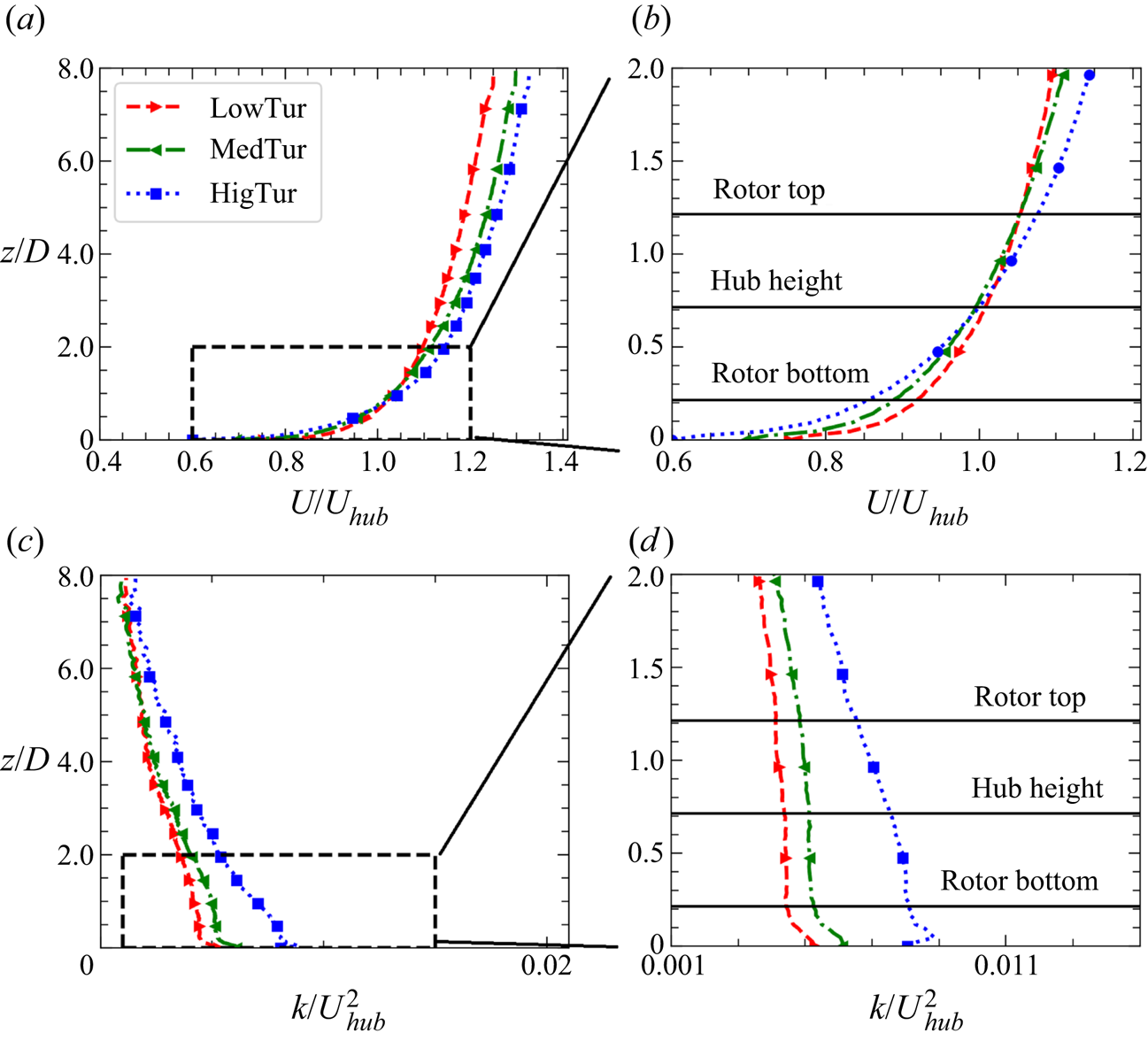
Figure 5. Vertical profiles of the time-averaged streamwise velocity (a), turbulent kinetic energy (c) and the corresponding zoomed-in view (b,d) across the rotor for different turbulent inflows.
In addition to the wind turbine wake cases, three no-turbine cases with the same computational set-ups are carried out to provide references for analysing the wake statistics. To obtain the time-averaged wake statistics, the flow fields are averaged for approximately  $400$ rotor revolutions after the flow is fully developed. A grid refinement study is carried out with the results presented in Appendix A, showing that the employed grid is capable of giving reliable predictions for the quantities of interest in this study. On the other hand, the employed grid is not enough for capturing the tip vortices in the near wake. To examine how different blade designs affect the structures of tip vortices, cases on a finer grid are carried out for the three blade designs under the LowTur inflow. The grid spacings are $\Delta x =D/60$ for $x \in [0, 2D]$ and $\Delta x =D/20$ for $x \in [3D, 12.5D]$, $\Delta y =D/120$ for $y \in [-1.5D, 1.5D]$ and $\Delta z =D/120$ for $z \in [0, 2D]$ with the number of grid nodes $N_x \times N_y \times N_z = 616 \times 501 \times 451$ in the three directions. The time step used in this finer grid is $0.00069D/U_{hub}$. Because of the high computational cost, only the instantaneous flow structures from the finer grid simulations are examined, without further averaging for computing the flow statistics.
4. Results
In this section, the results from the simulations of the three blade designs under three different inflows are compared and analysed, including the contours and profiles of wake statistics, the mean kinetic energy (MKE) budgets, the statistics of the instantaneous wake centres and the spectrum of velocity fluctuations.
The operational conditions of the wind turbine are presented in table 2 and figure 6. In table 2, the thrust coefficients ( $C_T=T/(0.5 \rho A U_{hub}^2)$, where $A = {\rm \pi}R^2$ and $T$ is the thrust) and the power coefficient ( $C_P=M \varOmega /(0.5 \rho A U_{hub}^3)$, where $M$ is the torque) are presented for the three blade designs. As seen, the three blade designs give the same $C_T$ for the same inflow as designed. As for the $C_P$, differences of around 5 % are observed. The radial distributions of the axial force coefficient ( $C_{F_a}$) from the three blade designs are compared in figure 6 for the LowTur inflow case, which is defined as
 \begin{equation} C_{F_a} = \frac{F_a}{\rho{\rm \pi} R U_{hub}^2}, \end{equation}
where  $F_a$ is the axial component of the force per unit length (in the radial direction) on the blade. It is seen that $C_{F_a}$ is higher near the blade root and tip regions for the NREL-Root and NREL-Tip designs, respectively, when compared with the NREL-Ori design.
Table 2. The thrust coefficient ( $C_T$) and power coefficient ( $C_P$) for the three blade designs under three different turbulent inflows.
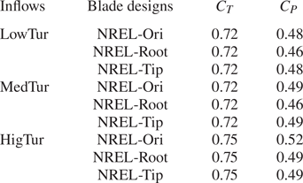

Figure 6. Radial distributions of the axial force coefficient ( $C_{F_a}$ in (4.1)) of the three blade designs for the LowTur inflow case.
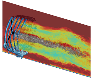
Before analysing the wake statistics, the instantaneous flow structures obtained from the finer grid simulations are examined in figure 7, which shows the tip vortices and hub vortex for the three blade designs under the LowTur inflow. It is seen that the hub vortex of the NREL-Root design is stronger than the other two designs, and expands to a much wider region as one travels in the downstream direction. The strength of the tip vortices of the NREL-Root design, on the other hand, is weaker than the other two designs. Overall, a rich dynamics is observed in the near-wake region. How this near-wake dynamics affects the wake statistics and the onset of wake meandering will be systematically examined in the rest of the paper.

Figure 7. Tip vortices and hub vortex for (a) the NREL-Ori, (b) the NREL-Root and (c) the NREL-Tip designs under the LowTur inflow. The tip vortices and the hub vortex are identified using the  $Q$ criterion ( $QD^2/U^2_{hub}=600$, where $Q = 0.5*(\boldsymbol{\varOmega}^2 - \boldsymbol{S}^2)$ ( $\varOmega$ is the vorticity tensor and $\boldsymbol{S}$ is the strain rate tensor) and the vorticity magnitude ( $|\omega |D/U_{hub}=90$), respectively.
4.1. Velocity deficits and turbulence statistics
In this part, the time-averaged velocity fields, TKE and the primary Reynolds shear stress are analysed for the three blade designs.
To get a first impression of how different blade designs affect the wake characteristics, figure 8 shows the contours of the time-averaged flow fields on the vertical plane passing through the rotor centre. It is seen from the first panel that, at the near wake locations, the streamwise velocity  $U/U_{hub}$ is the lowest for the NREL-Root design, and is the highest for the NREL-Tip design. For the NREL-Tip design, the lowest streamwise velocity is observed at locations close to the tip, with fairly high magnitudes of $U/U_{hub}$ at other vertical positions in the wake. In the second panel for the transverse velocity ( $V/U_{hub}$), which indicates the rotational motion of the wake, it is seen that the wake of the NREL-Root design loses such rotational motion faster when compared with the other two blade designs. At the very-near-wake locations ( $x/D<1$), the TKE ( $k/U_{hub}^2$) around the upper tip region is higher for the NREL-Tip design when compared with the other two designs, as shown in the third panel. At further downstream locations, the high TKE regions originating from the tip shear layer merge around the wake centreline, which happens earlier for the NREL-Root design compared with the other two designs, indicating the earlier onset of wake meandering for the NREL-Root design. Moreover, except at the near-wake locations, the magnitudes of TKE from the NREL-Root design are significantly higher. The last panel of figure 8 shows the contour of the primary Reynolds shear stress ( $\langle u'w' \rangle /U_{hub}^2$). Higher magnitudes of $\langle u'w'\rangle /U_{hub}^2$ are observed in wider regions along the top and bottom tips for the NREL-Root design when compared with the other two designs. The observations from the other two inflows are similar to those from the LowTur inflow, which are not shown here.

Figure 8. Time-averaged flow fields on the  $x$–
$x$– $z$ plane passing through the rotor centre in the wake of wind turbines with different blade designs under the LowTur inflow, with the first, second and third columns for the NREL-Ori, the NREL-Root and the NREL-Tip designs, respectively.
After having a view of the flow field for different blade designs, the vertical profiles of the time-averaged streamwise velocity deficit ( $\Delta U / U_{hub}$), the turbine-added turbulence kinetic energy ( $\Delta k /U_{hub}^2$) and the turbine-added primary Reynolds shear stress ( $\Delta \langle u^{\prime }w^{\prime } \rangle / U_{hub}^2$),
 $$\begin{gather} \Delta U = U_{NT} - U, \end{gather}$$
 $$\begin{gather}\Delta k = k -k_{NT}, \end{gather}$$
 $$\begin{gather}\varDelta \langle u'w'\rangle = \langle u'w' \rangle - \langle u'w' \rangle_{NT}, \end{gather}$$
where the subscript  $_{NT}$ denotes the quantities obtained in the simulation without a wind turbine, are analysed in figures 9, 10 and 11, respectively. From these figures, it is seen that the blade design is the most influencing factor affecting the downstream evolution of wind turbine wakes, especially at the near-wake locations ( ${<}4D$), with the vertical profiles of $\Delta U /U_{hub}$, $\Delta k /U_{hub}^2$ and $\varDelta \langle u^{\prime }w^{\prime }\rangle /U_{hub}^2$ from different inflows being similar to each other for the same blade design.

Figure 9. Vertical profiles of the time-averaged streamwise velocity deficit  $\Delta U /U_{hub}$ at different downstream locations for (a) LowTur, (b) MedTur and (c) HigTur inflows.

Figure 10. Vertical profiles of the turbine-added TKE  $\Delta k /U_{hub}^2$ at different downstream locations for (a) LowTur, (b) MedTur and (c) HigTur inflows.

Figure 11. Vertical profiles of the turbine-added primary Reynolds shear stress  $\varDelta \langle u'w' \rangle /U_{hub}^2$ at different downstream locations for (a) LowTur, (b) MedTur and (c) HigTur inflows.
We first probe into the effect of blade design on velocity deficit by examining figure 9. Besides the differences in the magnitude of velocity deficit shown in the first row of figure 8, the location for the maximal velocity is also different, that it is located approximately  $0.8R$ from the rotor centre for the NREL-Tip and NREL-Ori designs and approximately $0.5R$ for the NREL-Root design. At $2D$ to $4D$ downstream locations, the maximal velocity deficit is located close to the centreline, indicating the end of the near wake, which happens earlier for the NREL-Root design. At $6D$ downstream, the velocity deficits from the three designs are close to each other. At $12D$ downstream from the turbine, it is interesting to see that the velocity deficit from the NREL-Root design is somewhat lower than or comparable to the other two designs. It is noticed that the velocity deficit from the NREL-Root design is greater than the other two designs at the $1D$,
$1D$,  $2D$,
$2D$,  $3D$ and $4D$ downstream locations. That the velocity deficit from the NREL-Root design becomes comparable to and then lower than the other two designs at further downstream locations essentially means there is a faster recovery rate of the NREL-Root design, which is supported by the higher-magnitude TKE in the wake of the NREL-Root design and the analysis of the MKE budget carried out in § 4.2.
After showing the velocity deficit, how different blade designs affect the TKE in a wind turbine's wake is analysed in figure 10. As seen, the turbine-added TKE  $\Delta k /U_{hub}^2$ of the NREL-Tip design is higher than the other two designs at the $1D$ and $2D$ turbine downwind locations mainly in the top and bottom tip shear layers. At the $3D$ to $6D$ turbine downwind locations, on the other hand, $\Delta k /U_{hub}^2$ of the NREL-Root becomes the highest among the three designs. At $12D$ downstream, $\Delta k /U_{hub}^2$ of NREL-Root is still more or less the highest, especially for the MedTur inflow. In figure 11, similar trends are observed for the turbine-added primary Reynolds shear stress $\varDelta \langle u'w' \rangle /U_{hub}^2$, where the magnitude of $\varDelta \langle u'w' \rangle /U_{hub}^2$ of the NREL-Tip design is higher when compared with the other two designs at the $1D$ to $2D$ downstream locations, while at $3D$ to $5D$ downstream, the magnitude of $\varDelta \langle u'w' \rangle /U_{hub}^2$ of the NREL-Root design is the highest among the three designs.
To further show the downstream variations of the wake statistics, the streamwise variations of the time-averaged wake half-width  $R_{1/2}$ and the streamwise variations of the streamwise velocity ( $\langle U \rangle _d/U_{hub}$), pressure ( $\langle P-P_{0} \rangle _d /(0.5\rho U_{hub}^2)$, where $P_0$ is the pressure at the inlet located at hub height) and TKE ( $\langle k \rangle _d /U_{hub}^2$) averaged over time and a disk (of radius $R$ and its centre at rotor centreline) on the $y$–
$y$– $z$ plane at different turbine downwind locations are examined in figures 12 and 13, respectively. The wake half-width is obtained by fitting the Gaussian function as follows:
 \begin{equation} \Delta U(x,y) = \Delta U_c(x) \exp \frac{-(y-y_c(x))^2}{2\sigma(x)^2}, \end{equation}
where  $\Delta U(x,y)$ is the velocity deficit, $\Delta U_c(x)$ is the velocity deficit at the wake centre $y_c(x)$ and $\sigma (x)$ is the standard deviation of the Gaussian distribution. The wake half-width $R_{1/2}$ is defined as the distance from the wake centre to the position where $\Delta U = \frac {1}{2}\Delta U_c$, that is $R_{1/2}= \sqrt {2\ln 2} \sigma (x)$. The performance of fitting the instantaneous streamwise velocity deficit using the Gaussian function is examined in Appendix D.

Figure 12. Streamwise variations of time-averaged wake half-width  $R_{1/2}$ for (a) LowTur, (b) MedTur and (c) HigTur inflows.

Figure 13. Time- and disk-averaged streamwise velocity (a), pressure (b) and TKE (c) for different inflows.
It is seen in figure 12 that  $R_{1/2}$ from the NREL-Root design is larger than the other two designs in the far wake for all the three inflows, indicating a greater wake expansion in the spanwise direction. This is a result of stronger momentum mixing as shown in the TKE contours (figure 8) and indicates that the effect of wake-added turbulence should be accounted for in addition to the incoming turbulence when computing the wake radius at various downstream locations.
For the disk-averaged streamwise velocity, it is seen in figure 13(a) that it decreases to a much lower value at a further turbine downwind location for the NREL-Root design when compared with the other two designs. For the NREL-Tip design, the magnitude of the minimal streamwise velocity is slightly less and observed at a location slightly closer to the turbine when compared with those of the NREL-Ori design, indicating that the recovery of the NREL-Tip turbine wake is ahead of the other two blade designs. Although immediately behind the turbine, the streamwise velocity of the NREL-Root design is the smallest one, at  $7D$ downstream it recovers to almost the same as that of the other two blade designs, demonstrating that the recovery rate of the NREL-Root design is higher. By examining carefully the pressure variation on approaching the rotor in figure 13(b), it is seen that the pressure increase is higher for the NREL-Root design when compared with the other two designs. Simple calculations show that this pressure increase is approximately the same as the difference in the minimal streamwise velocity between the NREL-Root design and the other two designs. In the near wake, a further decrease of the streamwise velocity is related to the recovery of the pressure. It is seen in figure 13(b) that the pressure recovers at a lower rate for the NREL-Root design, which explains why the minimal streamwise velocity is observed at a further turbine downwind location for the NREL-Root design. As for the TKE $\langle k \rangle _d / U_{hub}^2$ shown in figure 13(c), it is observed that the maximal $\langle k \rangle _d / U_{hub}^2$ appears at a location closest to the turbine for the NREL-Tip design. The magnitude of the maximal $\langle k \rangle _d / U_{hub}^2$ of the NREL-Root design, on the other hand, is the largest among the three designs. For different inflows, similar trends are observed for all three quantities.
Overall, we have seen that the downstream extents influenced by the blade design are different for different quantities, with the differences in the streamwise velocity and the pressure mainly observed in the near wake ( $x \leqslant 4D\sim 6D$), and the differences in TKE and the wake half-width persisting even in the far wake. After showing the disk-averaged quantities, other near-wake features are further examined to understand the underlying flow physics. The momentum entrainment depends on the radial gradient of the streamwise velocity around the wake boundary. The downstream evolution of the streamwise velocity gradient in the spanwise direction ( ${\partial U}/{\partial y}$) at locations along the blade tip is examined in figure 14 for different blade designs. The most important observation in the very-near-wake region ( ${<}0.5D$) is that the magnitudes of ${\partial U}/{\partial y}$ from the NREL-Tip design are significantly higher than the other two designs, which is the major reason that the streamwise velocity recovers faster in the near wake and the maximum of $k$ is located closer to the turbine for the NREL-Tip design. At further turbine downwind locations ( $1D< x<3D$), the magnitudes of ${\partial U}/{\partial y}$ from the three designs are similar to each other. The effects of blade designs on ${\partial U}/{\partial y}$ are similar for different inflows.

Figure 14. Streamwise variations of the spanwise gradient of the time-averaged streamwise velocity for (a) LowTur, (b) MedTur and (c) HigTur inflows.
The tip shear layer expands and meets at the wake centreline, after which the wake may start the meandering motion. Here, we employ the distance between the two peaks of the streamwise velocity deficit in the spanwise direction, i.e.  $d_{2p}$ as shown in figure 15 to measure the downstream evolution of the tip shear layer. As shown in figure 15, $d_{2p}$ first remains roughly the same for the NREL-Ori and NREL-Tip designs while it increases for the NREL-Root design, and then gradually decreases to zero at further turbine downwind locations. Compared with the NREL-Ori design, $d_{2p}$ of the NREL-Tip design is larger and starts to decrease at a further turbine downwind location. The downstream distance where $d_{2p}$ decreases to zero is the longest for the NREL-Tip design, indicating the possible late onset of wake meandering for this design.

Figure 15. Evolution of the tip shear layer for different inflows (a) the LowTur, (b) the MedTur and (c) the HigTur inflows in the horizontal  $x$–
$x$– $y$ plane at $z = z_{hub}$ along different downwind positions. The inset in (a) shows the spanwise profile of the streamwise velocity deficit at $1D$ downstream with the turbine located $y=0$. The red circle, green square and blue triangle symbols represent the results of the NREL-Ori, the NREL-Root and the NREL-Tip designs, respectively.
4.2. Budget of the MKE
In this section, the budget equation of MKE is analysed, which can be written as follows:
 \begin{align} 0 & =-\langle u_j \rangle
\frac{\partial \langle u_i \rangle \langle u_i \rangle
/2}{\partial x_j} - \frac{\partial}{\partial x_j} \left (
\frac{1}{\rho} \langle p \rangle \langle u_j \rangle +
\langle u_i^{'} u_j^{'} \rangle \langle u_i \rangle - 2(\nu
+\nu_t){\mathsf{S}}_{ij}\langle u_i \rangle \right )\nonumber\\ &\quad
+ \langle u_i^{\prime} u_j^{\prime} \rangle \frac{\partial
\langle u_i \rangle}{\partial x_j} - 2(\nu
+\nu_t){\mathsf{S}}_{ij}\frac{\partial \langle u_i \rangle}{\partial
x_j} . \end{align}
\begin{align} 0 & =-\langle u_j \rangle
\frac{\partial \langle u_i \rangle \langle u_i \rangle
/2}{\partial x_j} - \frac{\partial}{\partial x_j} \left (
\frac{1}{\rho} \langle p \rangle \langle u_j \rangle +
\langle u_i^{'} u_j^{'} \rangle \langle u_i \rangle - 2(\nu
+\nu_t){\mathsf{S}}_{ij}\langle u_i \rangle \right )\nonumber\\ &\quad
+ \langle u_i^{\prime} u_j^{\prime} \rangle \frac{\partial
\langle u_i \rangle}{\partial x_j} - 2(\nu
+\nu_t){\mathsf{S}}_{ij}\frac{\partial \langle u_i \rangle}{\partial
x_j} . \end{align}
To facilitate the analysis of the wake as a whole, (4.6) is integrated into the spanwise and vertical directions from  $y_1=y_c-R$ to $y_2=y_c+R$ and $z_1 =z_{hub}-R$ to $z_2=z_{hub}+R$. The integral form of the MKE equation is in the following form:
 \begin{equation} 0 = MC + PT + TC + DF + TP + DP, \end{equation}
where
 $$\begin{gather} MC =-\int_{y_1}^{y_2} \int_{z_1}^{z_2} \langle u_j \rangle \frac{\partial \left ( \langle u_i \rangle \langle u_i \rangle /2 \right )}{\partial x_j}\,{\rm d}z\,{{\rm d}y}, \end{gather}$$
 $$\begin{gather}PT =-\int_{y_1}^{y_2} \int_{z_1}^{z_2} \langle u_j \rangle \frac{\partial \left ( \langle p \rangle \langle u_j \rangle /\rho \right )}{\partial x_j}\,{\rm d}z \,{{\rm d}y}, \end{gather}$$
 $$\begin{gather}TC =-\int_{y_1}^{y_2} \int_{z_1}^{z_2} \frac{\partial \left ( \langle u_i^{\prime} u_j^{\prime} \rangle \langle u_i \rangle \right )}{\partial x_j}\,{\rm d}z \,{{\rm d}y}, \end{gather}$$
 $$\begin{gather}DF = 2\int_{y_1}^{y_2} \int_{z_1}^{z_2} \frac{\partial \left ( \nu + \nu_t \right ) {\mathsf{S}}_{ij}\langle u_i \rangle}{\partial x_j}\,{\rm d}z \,{{\rm d}y}, \end{gather}$$
 $$\begin{gather}TP = \int_{y_1}^{y_2} \int_{z_1}^{z_2} \langle u_i^{\prime} u_j^{\prime} \rangle \frac{\partial \langle u_i \rangle}{\partial x_j}\,{\rm d}z\,{{\rm d} y}, \end{gather}$$
 $$\begin{gather}DP =-2\int_{y_1}^{y_2} \int_{z_1}^{z_2} \left ( \nu + \nu_t \right ) {\mathsf{S}}_{ij} \frac{\partial \langle u_i \rangle}{\partial x_j}\,{\rm d}z\,{{\rm d}y}. \end{gather}$$
In the above equations,  $MC$,
$MC$,  $PT$,
$PT$,  $TC$,
$TC$,  $DF$,
$DF$,  $TP$ and $DP$ represent the mean convection term, the pressure transport term, the turbulent convection term, the diffusion term, the turbulence production term and the dissipation term, respectively.
Figure 16 compares different terms of the MKE budget equation for different designs. It is seen that the blade design is the key factor affecting the streamwise variations of different terms in the MKE budget equation, which are similar to each other for different inflows when the blade design is the same. For all the cases, it is seen that, in the very near wake ( $x< 1D \sim 2D$), the mean convection term $MC$ is mainly balanced by the pressure transport term $PT$, in which the latter extracts energy from the MKE as the pressure behind the turbine recovers. In the far wake ( $x>3D \sim 5D$), the $MC$ term and the turbulence convection term $TC$ are the two leading terms, in which the $TC$ term plays a key in the recovery of the far wake.

Figure 16. The MKE budget for different blade designs under different turbulent inflow conditions. The MKE budget terms are normalized using  $U_{hub}$ and $D$.
$D$.
To further probe into the effects of blade design on the processes involved in the evolution of MKE, the  $MC$,
$MC$,  $PT$,
$PT$,  $TC$ and $TP$ terms are examined separately in figure 17. It is seen in figure 17(a) that the $MC$ term decreases to zero at approximately $1.5D$ downstream for both the NREL-Ori and NREL-Tip designs, while for the NREL-Root design, it decreases mildly after $x=1D$ downstream and approaches zero at approximately $2.5D$ downstream. From the pressure transport term $PT$ shown in figure 17(b), it is seen that the $PT$ term decreases to a negative value of lower magnitude for the NREL-Root design when compared with the other two designs. This shows that less energy is extracted from the MKE for the NREL-Root design as the pressure recovers in the near wake. As seen in figure 17(c), the peak of the $TC$ term of larger magnitude appears at a location closer to the turbine for the NREL-Tip design when compared with the other two designs, which, on the other hand, appears at a further downstream location at a higher magnitude for the NREL-Root design when compared with the NREL-Ori design. This explains the faster wake recovery at locations closer to the turbine for the NREL-Tip design, and the faster wake recovery in the far wake for the NREL-Root design. The $TP$ term, being the source term for TKE, is examined in figure 17(d). It is seen that the maxima of the magnitude of the $TP$ term from the NREL-Tip and NREL-Root designs are higher and appear at a location closer to and further from the turbine, respectively when compared with the NREL-Ori design.

Figure 17. Mean convection ( $MC$), pressure transport ( $PT$), turbulence convection ( $TC$) and turbulence production ( $TP$) terms of the MKE budget equation for (a) LowTur, (b) MedTur and (c) HigTur inflows.
4.3. Statistics of wake meandering
In this section, the characteristics of wake meandering are analysed by examining the statistics of instantaneous wake centres and the power spectrum of velocity fluctuations at different turbine downwind locations.
The centre of the instantaneous wake is extracted by fitting a Gaussian function, in the same way as for the time-averaged wake. The contours of the instantaneous streamwise velocity deficit together with the instantaneous wake centre and half-width from different designs are shown in figure 18 at exactly the same time instant. It is seen that the wake centre is located closer to the centreline in the near wake and meanders significantly in the far wake. Such meandering motion is observed starting earlier for the case with high inflow turbulence intensity (i.e. HigTur).

Figure 18. Instantaneous wake centres and half-width overlaid on contours of the instantaneous streamwise velocity deficit ( $\Delta u/U_{hub}$) on the $x$–
$x$– $y$ plane at $z = z_{hub}$ for (a) LowTur, (b) MedTur and (c) HigTur inflows. The black dashed lines represent the wake centre, and the black solid lines represent the wake half-width, respectively.
With the instantaneous wake centres  $y_c$, the downstream variations of the standard deviations ( $\sigma _{y_c}$) of $y_c$ from different blade designs are compared in figure 19. For all the inflows, it is seen that, from $0$ to $3D$ downstream, the values of $\sigma _{y_c}$ from different blades are close to each other. At further downstream locations, the values of $\sigma _{y_c}$ from the NREL-Root design are significantly higher than the other two designs, indicating that the meandering amplitude of this design is larger than that of the other two designs.

Figure 19. Standard deviations of instantaneous spanwise wake position  $y_c$ for (a) LowTur, (b) MedTur and (c) HigTur inflows.
To further examine the effect of blade design on the meandering motion at different scales, the time series of the instantaneous wake centres are decomposed into the low-frequency part  $y_{c1}$ with $St < 0.1$ and the high-frequency part $y_{c2}$. After the decomposition in the frequency space, an inverse fast Fourier transform (FFT) is conducted to obtain the time series of $y_{c1}$ and $y_{c2}$. As the Strouhal number of the wake meandering due to the shear layer instability is larger than 0.1 (Heisel et al. Reference Heisel, Hong and Guala2018; Yang & Sotiropoulos Reference Yang and Sotiropoulos2019b; Li et al. Reference Li, Dong and Yang2022), the low-frequency part $y_{c1}$ represents the influence from the inflow large eddies. Figures 20 and 21 show the thus-obtained time series of $y_{c1}$ and $y_{c2}$ at $3D$ and $12D$ downstream under the LowTur inflow. It is seen that at both locations the large-scale patterns shown in the time series of $y_{c1}$ from the three designs are approximately the same for the same inflow, while the variations of $y_{c2}$ are fairly chaotic and differ significantly between different blade designs. For both components of fluctuating wake centre positions, the magnitudes at $3D$ downstream are significantly lower than those at $12D$ downstream. With the time series of $y_{c1}$ and $y_{c2}$, their root mean square (r.m.s.) are computed and plotted in figure 22. It is seen that the values of r.m.s. of $y_{c1}$ of the low-frequency components from different blade designs are close to each other (figure 22a), while those of the high-frequency components from the NREL-Root design are higher than the other two designs, with a maximum difference 10 % to 20 %.

Figure 20. Temporal variations of instantaneous spanwise wake centre positions under the LowTur inflow at  $3D$ downstream for (a) $y_c$ of all resolved frequencies, (b) $y_{c1}$ of the low-frequency part with $St < 0.1$ and (c) $y_{c2}$ of the high-frequency part. The value of $t$ is normalized by using $D$ and $U_{hub}$, i.e. $T={D}/{U_{hub}}$.

Figure 21. Temporal variations of instantaneous spanwise wake centre positions under the LowTur inflow at  $12D$ downstream for (a) $y_c$ of all resolved frequencies, (b) $y_{c1}$ of the low-frequency part with $St < 0.1$ and (c) $y_{c2}$ of the high-frequency part. The $t$ is normalized by using $D$ and $U_{hub}$, i.e. $T={D}/{U_{hub}}$.

Figure 22. R.m.s. of instantaneous spanwise wake centre positions for (a) the low-frequency part  $y_{c1}$ and (b) the high-frequency part $y_{c2}$.
As exactly the same time series of inflow is fed at the inlet for different blade designs, it is then feasible to examine the correlation between the instantaneous wake centres between different designs. In figure 23, the correlation coefficients between the NREL-Tip and NREL-Ori designs and the NREL-Root and NREL-Ori designs are plotted for the spanwise wake centre fluctuations of all resolved frequencies ( $y_{c}$), of the low-frequency component ( $y_{c1}$) and of the high-frequency component ( $y_{c2}$). As seen, the correlation coefficient for $y_c$ gradually decreases as one travels in the downstream direction, especially for the HigTur inflow. The correlation coefficient for $y_{c1}$ is close to one for $x/D<8$ for the MedTur and HigTur inflows, and close to one even at $x/D=12$ for the LowTur inflow. The correlation coefficient for $y_{c2}$, on the other hand, decreases to a value ${\sim }0.5$ for the LowTur and MedTur inflows, and to a value ${\sim }0.25$ at $x/D=12$ for the HigTur inflow.

Figure 23. Correlation coefficients of the instantaneous spanwise wake positions between the NREL-Root and NREL-Ori designs (the red lines), and the NREL-Tip and NREL-Ori designs (the green lines) for (a)  $y_c$, (b) $y_{c1}$ and (c) $y_{c2}$.
Hereafter, the frequency features of wake meandering are examined by analysing the pre-multiplied power spectra of the spanwise velocity fluctuations ( $\,f\phi _v$) at two radial locations, i.e. $y=0$ and $y=R$. As shown in figure 24 for the results from the LowTur inflow cases, one major difference is that the high energy contents first appear at the blade tip for the NREL-Ori and NREL-Tip designs, and around the wake centreline for the NREL-Root design. For the NREL-Ori and NREL-Tip designs, the coherent motion within the tip shear layer ( $y=R$) at $x/D=1, 2$ appears at a frequency with $St$ in the range of 1 to 2, with the corresponding magnitude from the NREL-Tip design significantly higher. At further downstream locations, the magnitude of $f\phi _v$ with $St \in (1,2)$ decreases, while the wake meandering motion with $St$ approximately $0.4 \sim 0.6$ shows up for the entire wake starting from $x/D$ around $3$ and $4$ for the NREL-Ori and NREL-Tip designs. The scenario of the NREL-Root design is different, in that the coherent motion with a high magnitude of $f\phi _v$ first appears at the centreline $y=0$ at $x/D=1$. At $x/D=2$, the meandering motion with $St$ around $0.3\sim 0.4$ shows up at both the wake centreline and the tip layer for the NREL-Root design. Within the tip shear layer, the coherent motion with $St \in (1,2)$ appears at $x/D=2$ for the NREL-Root design, with the magnitudes lower than the NREL-Ori and NREL-Tip designs. For the MedTur and HigTur inflow cases, similar trends are observed (results not shown here).

Figure 24. The pre-multiplied power spectra of the spanwise velocity fluctuations at different downstream locations for the LowTur inflow.
To further analyse the genesis of the wake meandering for different blade designs, the statistics of power spectral density (PSD) at different spatial locations are further examined. The examined PSD statistics include the dominant frequency ( $\,f_c$) and the first moment of PSD about the dominant frequency ( $M_1(S_v)$). The dominant frequency is defined as the centre of mass of PSD as follows:
 \begin{equation} f_c = \frac{\displaystyle\int\nolimits_{f_{min}}^{f_{max}} f S_v(\,f) \,{\rm d}f}{ \displaystyle\int\nolimits_{f_{min}}^{f_{max}} S_v(\,f) \,{\rm d}f}. \end{equation}
The first moment of PSD is computed by
 \begin{equation} M_1(S_v) = \frac{\displaystyle\int\nolimits_{f_{min}}^{f_{max}} {S_v|f -f_c|\,{\rm d}f}}{f_{max}-f_{min}}. \end{equation}
Defining the dominant frequency using (4.14) is to avoid the ambiguity of defining it using the frequency of the maximum PSD. The first moment of PSD, on the other hand, provides a way to measure the distribution of high-amplitude PSD. Considering two PSDs (i.e.  $S_{v1}$ and $S_{v2}$) with the same TKE (i.e. $\int _{f_{min}}^{f_{max}} {S_v\,{\rm d}f}$ is the same), if $M_1(S_{v1})>M_1(S_{v2})$, then the high-amplitude PSD is distributed in a wider spectral width for $S_{v1}$.
The Strouhal number  $St_c$ of the dominant frequency $f_c$ is shown in figure 25. It is seen that the contour of $St_c$ can be divided into two regions, the tip layer region of high frequency and the inner layer region of low frequency. As one travels in the downstream direction, the width of the tip layer region increases. It is seen that the inner layer region of low frequency dominates for a longer distance for the NREL-Root design when compared with the other two designs. For the NREL-Tip design, on the other hand, the tip layer region of high frequency dominates. The interplay of the hub vortex and tip shear layer triggers the wake meandering of the shear layer instability type for the three designs. The relative strength of the turbulence structures in the tip shear layer and the hub vortex, on the other hand, determines the dominant frequency of wake meandering.

Figure 25. Contours of the dominant frequency  $St_c$ (4.14) on the $x$–
$x$– $y$ plane for (a) the LowTur, (b) the MedTur and (c) the HigTur inflows.
The first moment of PSD about  $f_c$ ( $M_1$ defined in (4.15)) is shown in figure 26. It is observed that the overall patterns of $M_1$ from the three blade designs are similar, that the high-magnitude $M_1$ originates from the tip shear layer and expands to the whole wake region at further downstream locations. The differences of $M_1$ for different blade designs lie in the starting position, the streamwise extent and the magnitude of high-magnitude $M_1$. The high-magnitude $M_1$ of the NREL-Tip design starts earlier when compared with the other two designs. The high-magnitude $M_1$ of the NREL-Root design, on the other hand, starts the latest but is of higher magnitude and resides in a longer region when compared with the other two designs. Moreover, it is seen that increasing the inflow turbulence intensity increases the $M_1$ magnitude and the streamwise extent of the high-magnitude $M_1$ region for the three blade designs.

Figure 26. Contours of the first moment of PSD ( $M_1$ in (4.15)) on the $x$–
$x$– $y$ plane for (a) the LowTur, (b) the MedTur and (c) the HigTur inflows.
5. Conclusions
In this work, the effects of blade designs on the characteristics of wind turbine wakes were systematically investigated using LES with the blade and nacelle modelled using the AS model. Three different blade designs with approximately the same thrust coefficient were employed, i.e. the blade design of the NREL 5 MW baseline offshore wind turbine (NREL-Ori), and the NREL-Root and NREL-Tip designs (two variants of the NREL-Ori design) with higher load near the blade root and tip, respectively. For each blade design, three turbulent inflows corresponding to three different ground roughness lengths, i.e.  $k_0=0.001, 0.01, 0.1$ m, were considered.
The blade design affects the wake characteristics in both the near-wake and far-wake regions as shown by the simulation results. Significant differences in the streamwise velocity deficit ( ${>}10$ % of the incoming wind speed $U_{hub}$) are observed between different blade designs until $5D$ downstream. In the near wake, the magnitude of the streamwise velocity deficit is the largest for the NREL-Root design, mainly caused by the higher pressure increase as the incoming flow approaches the rotor when compared with the other two designs. However, the wake recovery rate of the NREL-Root design is the highest, which is a result of lower loss in pressure transport and greater gain in turbulence convection as shown by the analysis of the budget equation of the mean kinetic energy. As for the TKE, the magnitude of the maximum from the NREL-Tip design is the largest in the near wake ( $x/D<2$), which is caused by the high magnitude of the velocity gradient in the radial direction. The magnitude of the maximal turbulence kinetic energy from the NREL-Root design, on the other hand, is larger than the other two designs at further downstream locations, where the wake meandering is prevalent.
The blade design affects the wake meandering. The simulation results show that the amplitude of wake meandering (i.e. the standard deviations of the instantaneous spanwise wake positions) from the NREL-Root design is higher than the other two designs. Further analysis, in which the time series of the instantaneous wake centre positions are decomposed into the low-frequency component ( $St < 0.1$) and the rest high-frequency component, to examine the influence of the inflow of large eddies and the shear layer instability is carried out. The obtained results show that the major difference lies in the high-frequency component, which is induced by the shear layer instability, for different blade designs. Analysis of the spectra of the velocity fluctuations shows different roles of the tip shear layer and hub vortex in wake meandering, that the former sets the starting position for the development of wake meandering and the interaction between the two determines the dominant frequency and the intensity of wake meandering. The stronger the tip shear layer, the earlier the starting position; the stronger the hub vortex, the lower the meandering frequency and the higher the amplitude of wake meandering. Such a meandering mechanism is confirmed by the facts that the meandering frequency of the NREL-Root design is lower than the other two designs, and the meandering amplitude of the NREL-Tip design is somewhat higher in the near wake when compared with the other two designs. Furthermore, the differences observed in the far wake indicate that the assumption often made in analytical wake models, that the far-wake statistics only depend on the integral-form coefficients, like the thrust coefficient and the power coefficient, needs to be revisited if one wants to account for the effects of blade designs. One limitation of the present work is that the aeroelasticity was not considered, which can be accounted for using the latest version of the VFS-Wind code, which couples the AS model with an aeroelastic model (Santoni et al. Reference Santoni, Khosronejad, Yang, Seiler and Sotiropoulos2023).
From a practical point of view, the motivation of this work is to explore the potential of improving the performance of the entire wind farm by placing wind turbines of different blade designs at different positions. A proof-of-concept study in a virtual simulation environment will be carried out in future work. Two important issues, i.e. the complexity of real-life wind conditions and the high computational cost of high-fidelity simulations, need to be addressed properly to develop this type of wind farm design strategy. The first issue involves the effects of complex terrain, unsteady wind condition, thermal stratification and others. A thorough understanding of the wake dynamics of different blade designs under different wind conditions is required to set the theoretical basis for such development. Analytical wake models and data-driven wake models considering the effects of blade designs need to be developed to avoid the need for running high-fidelity simulations in the design process. Overall, the development of turbine placement strategies with the consideration of blade designs is still at a very early stage and requires lots of fundamental studies from the fluid mechanics aspect.
Funding
This work was funded by the NSFC Basic Science Center Program for ‘Multiscale Problems in Nonlinear Mechanics’ (No. 11988102), National Natural Science Foundation of China (No. 12172360, 12202456, and 12202453), Institute of Mechanics CAS and Chinese Academy of Sciences.
Declaration of interests
The authors report no conflict of interest.
Appendix A. Grid refinement study
A grid refinement study is performed for three different grid resolutions, i.e. the coarse, medium and fine grids shown in table 3, for the NREL-Root blade design under the LowTur inflow. The medium grid is employed for most analyses carried out in this study except for the examination of vortex structures in the near wake (figure 7), for which a grid finer than the fine grid shown in table 3 is employed. In the  $x$ direction, the grid nodes are uniformly distributed for the coarse and the medium grids. For the fine grid, the grid nodes are uniformly distributed with $\Delta x = D/40$ in the near wake until $x=2D$ downstream, gradually stretched to $\Delta x = D/20$ at $x=3D$ and placed at a constant grid spacing with $\Delta x = D/20$ at further downstream locations. In the $y$ direction, the grid nodes are uniformly distributed for the coarse and the medium grids. For the fine grid, the grid nodes are uniformly distributed with $\Delta y = D/80$ for $y\in [-1.5D, 1.5D]$ and gradually stretched to the left and right boundaries. In the $z$ direction, the grid is uniform for $z\in [0, 2.0D]$ and gradually stretched to the top boundary.
Table 3. Grid spacings and the number of grid nodes for the three grids employed for the grid refinement study.
The vertical profiles of the streamwise velocity and TKE are shown in figure 27. An overall good agreement is observed between the predictions from the medium and the fine grids for both quantities. The standard deviations of instantaneous wake positions ( $\sigma _{yc}$) from the three grids are examined in figure 28. An overall good agreement among the three grids is observed, except in the far wake, where the $\sigma _{yc}$ predicted by the coarse grid is different from those for the other two grids.

Figure 27. Vertical profiles of (a) the time-averaged streamwise velocity and (b) the TKE computed from the coarse, the medium and the fine grids. The NREL-Root blade design under the LowTur inflow is employed.

Figure 28. Standard deviations of instantaneous wake centre positions in the spanwise direction computed from the three grids. The NREL-Root blade design under the LowTur inflow is employed.
Appendix B. Generation of turbulent inflows
The turbulent inflows are generated from precursory simulations, in which the periodic boundary conditions are applied in the horizontal directions, the free-slip boundary condition is applied at the top boundary and the wall model with wall shear stress computed from the logarithmic law for a rough wall is applied at the bottom boundary. Three different ground roughness lengths, i.e.  $z_0 = 0.001\ \textrm {m}$, $0.01\ \textrm {m}$, $0.1\ \textrm {m}$ corresponding to the LowTur, the MedTur and the HigTur inflows, are considered. The size of the computational domain is $L_x \times L_y \times L_z = 22.5 \delta \times 14.88\delta \times \delta$, where $\delta =1$ km is the thickness of the ABL, with the corresponding number of grids $N_x \times N_y \times N_z = 1126 \times 1488 \times 152$. In the $x$ and $y$ directions, the grid nodes are uniformly distributed. In the $z$ direction, the grid is uniform for $z\in [0, 0.15\delta ]$ with a grid spacing $\Delta z = 0.002\delta$, and gradually stretched to the top boundary.
The grid employed in the precursory simulation is different from that of wind turbine wake simulations on the  $y$–
$y$– $z$ plane. The size of the time step is different as well. Linear interpolation in both time and space is employed to obtain the inflow for the wind turbine wake simulations. It is noted that the spanwise dimension of the computational domain employed in the precursory simulation is larger than the wind turbine wake simulation. Only a fraction of the flow field from the precursory simulation is employed for generating the inflow.
Appendix C. Wake statistics of a different tip-loaded blade design
This appendix is to show that the wake of the NREL-Tip design is representative of the tip-loaded type blade designs, even though the chord distribution in the root region may have structural issues. The approach is to design a blade with a radial distribution of the axial force coefficient similar to the NREL-Tip design by only adjusting the twist of the NREL-Ori design (the NREL-Tip-OnlyTwist design) and compare the wake statistics from the two blade designs.
Figure 29 shows the radial distributions of the twist and chord from the NREL-Ori, NREL-Tip and NREL-Tip-OnlyTwist designs. The radial distributions of the obtained axial force coefficients ( $C_{F_a}$) are examined in figure 30, showing similar radial distributions of $C_{F_a}$ of the NREL-Tip and NREL-Tip-OnlyTwist designs. Figures 31 and 32 present the time-averaged streamwise velocity and TKE from the NREL-Tip and the NREL-Tip-OnlyTwist blade designs. Overall, the wake statistics from the two designs are very similar to each other, except for very minor differences observed in the near wake.

Figure 29. Radial distributions of twist and chord from the NREL-Ori, NREL-Tip and NREL-Tip-OnlyTwist designs.

Figure 30. Radial distributions of the axial force coefficient  $C_{F_a}$ for the NREL-Ori, NREL-Tip and NREL-Tip-OnlyTwist designs.

Figure 31. Contours of the time-averaged streamwise velocity for the NREL-Tip and the NREL-Tip-OnlyTwist blade designs (a,c) and the TKE for the NREL-Tip and the NREL-Tip-OnlyTwist blade designs (b,d).

Figure 32. Vertical profiles of (a) time-averaged streamwise velocity and (b) TKE from the NREL-Tip and NREL-Tip-OnlyTwist blade designs.
This appendix proves that the wake statistics of the NREL-Tip design are representative of the tip-loaded blade designs with similar axial force coefficients. Whether the distribution of  $C_{F_a}$ is designed by adjusting the chord or twist is not significant for the wake statistics examined in this work.
Appendix D. Gaussian fitting of instantaneous streamwise velocity profiles
The performance of fitting the instantaneous streamwise velocity using the Gaussian function is examined in this appendix.
A comparison of the original velocity deficit profiles and the fitted ones is shown in figure 33. Deviations from the Gaussian function are observed at both near-wake and far-wake positions, which is mainly due to the less-developed state of the wake and turbulent fluctuations, respectively.

Figure 33. Comparison of the Gaussian fitted and the original spanwise profiles (without fitting in space) of the instantaneous streamwise velocity deficit at  $1D$ (a) and $12D$ (b) downstream for the three blade designs.
There is a chance that the Gaussian function may fail to fit the instantaneous streamwise velocity deficit profiles. To reduce such a chance, the instantaneous profiles are first filtered in the streamwise direction using a box filter of width  $0.5D$ in this work. To evaluate the performance of the two approaches with and without spatial filtering, the fitting error $e_{u_{fit}}$, which is defined as the root-mean-square of the difference between the fitted velocity $u_{fit}$ and the real velocity $u$, is examined. The streamwise variations of the error in velocity fitting are depicted in figure 34. The error is higher in the near-wake region. It is clear that the fitting error at both near-wake and far-wake positions can be reduced significantly with spatial filtering.

Figure 34. The errors between the standard deviation of the no-filtering wake centre position and of the spatial filtering wake centre position for (a) LowTur, (b) MedTur and (c) HigTur inflows.
Filtering the velocity in space reduces the error of fitting the instantaneous velocity using the Gaussian function. On the other hand, it may reduce the small-scale fluctuations of instantaneous wake positions, possibly increasing the error of wake centreline position. Based on the results presented in this appendix, also considering that the wake meandering motion is of major concern in this work, spatial filtering is carried out before the velocity fitting using the Gaussian function.


