


1. Introduction
Morphology of leg structures is fundamental to leg locomotion. A well-designed leg will enable the system to locomote with less energy dissipation and simplify the control of interactions with irregular terrains. Nowadays, most legged robots use the simple morphology of two-link structure as their leg designs, in which the upper limb and the lower limb are connected in series. Humanoid robots such as Atlas [1], Valkyrie [Reference Radford, Strawser, Hambuchen, Mehling, Verdeyen, Donnan, Holley, Sanchez, Nguyen, Bridgwater, Berka, Ambrose, McQuin, Yamokoski, Hart, Guo, Parsons, Wightman, Dinh, Ames, Blakely, Edmonson, Sommers, Rea, Tobler, Bibby, Howard, Nui, Lee, Conover, Truong, Chesney, Platt, Johnson, Fok, Paine, Sentis, Eric, Sinnet, Lack, Powell, Morris and Ames2], and HRP [Reference Kajita, Benallegue, Cisneros, Sakaguchi, Morisawa, Kaminaga, Kumagai, Kaneko and Kanehiro3], quadruped robots such as HyQ [Reference Semini, Barasuol, Focchi, Boelens, Emara, Casella, Villarreal, Orsolino, Fink, Fahmi, Medrano-Cerda, Caldwell, Sangiah, Lesniewski, Fulton, Donadon and Baker4], ANYmal [Reference Gehring, Fankhauser, Isler, Diethelm, Bachmann, Potz, Gerstenberg and Hutter5], and MIT mini Cheetah [Reference Katz, Di Carlo and Kim6] use this type of leg structure. Elastic elements are usually excluded in such two-link leg structure, which makes it sensitive to impacts and inefficient in energy recycling. However, due to the simple transmission mechanism of this structure, the robot system is more practically reliable and is easier to apply force control on the end effector.
Despite all the advantages that the rigid two-link leg structure has, leg elasticity is discovered to enhance locomotion performance in terms of stability, robustness, impact mitigation, and simplify the control task [Reference Beckerle, Verstraten, Mathijssen, Furnémont, Vanderborght and Lefeber7–Reference Verstraten, Beckerle, Furnémont, Mathijssen, Vanderborght and Lefeber10]. Following an engineering constructive leg design framework, the primary focus in designing leg elasticity has been on virtual leg axis direction compliance, aiming at matching the spring-loaded inverted pendulum or spring-mass template [Reference Rezazadeh, Abate, Hatton and Hurst11]. Among different studies, Biped robot ATRIAS uses a four-bar series-elastic leg design to replicate the human-like ground-reaction forces of spring-mass walking [Reference Hubicki, Grimes, Jones, Renjewski, Spröwitz, Abate and Hurst12]. It is capable of achieving running, variable speed control, blindly traversing over obstacles, and recovering from strong human kicks [Reference Hubicki, Abate, Clary, Rezazadeh, Jones, Peekema, Van Why, Domres, Wu, Martin, Geyer and Hurst13]. It owes its dynamical capabilities to its spring-mass design approach, which regulates the dynamics of the robot system, making it predictable by simple model, and finally improves the control performance [Reference Hubicki, Grimes, Jones, Renjewski, Spröwitz, Abate and Hurst12]. However, this four-bar series-elastic leg design has the flaw of antagonistic work loop, where one of the motors has to apply negative power during walking or running and causes the waste of energy [Reference Rezazadeh, Abate, Hatton and Hurst11]. Biped robot Cassie overcame this problem by altering the actuator placement and embedding the elastic elements (leaf springs) into two linkages of the four-bar structure [Reference Abate14]. It achieves dynamic walking and running and is able to handle diverse and complex terrains [Reference Chen and Posa15, Reference Gong, Hartley, Da, Hereid, Harib, Huang and Grizzle16].
On the contrary to aforementioned engineering leg design procedure, a lot of studies investigate biologically inspired leg designs. Among different designs, the pantograph structure gained widespread attention [Reference Witte, Hackert, Lilje, Schilling, Voges, Klauer, Ilg, Albiez, Seyfarth, Germann, Hiller, Dillmann and Fischer17]. It extracts main mammalian leg features, like three-segmentation, segment alignment, and compliant elements. Quadruped robot Cheetah-cub improved the pantograph structure by adding a diagonal spring and a second spring. It achieves fast running gait and shows self-stabilizing behavior over a range of speeds with open-loop control [Reference Spröwitz, Tuleu, Vespignani, Ajallooeian, Badri and Ijspeert18]. Bi-articular muscle-tendon structure [Reference Ruppert and Badri-Spröwitz19] is another leg design based on the pantograph structure. It adds one spring around the knee joint and a bi-articular spring in one of the linkage. This structure has both virtual leg axis and leg angle compliance. Experiments show that this design reduces energy requirements and cost of transport by 31% during dynamic hopping [Reference Ruppert and Badri-Spröwitz19]. However, most pantograph structure-based compliant leg designs, due to their complex spring configuration and cable-driven mechanism, are not suitable for composing a legged robot system.
In this paper, we characterize one compliant leg design that based on the conventional pantograph structure but enhanced by two linkage-embedded leaf springs. Main advantages of the proposed design are listed as follows:
-
1. The proposed compliant leg design owes more flexibility in altering the system stiffness due to using leaf springs. Compared with coil springs, leaf springs are bidirectional twist-able, easier to deploy, and their stiffness can be easily altered by adjusting their width, length, or thickness.
-
2. Compared with the conventional rigid pantograph structure, the proposed leg mechanism consists of two unparalleled leaf springs, which can estimate the contact forces and passively save the impact energy during leg locomotion.
-
3. Based on the proposed design, the one-leg compliant robot owes some good properties for legged locomotion: simple to build, centralized mass around its hip joint, and capable of estimating the contact forces only with leaf springs’ deflection.
The rest of the paper is organized as follows: In Section 2I, we introduce the proposed leg design and analyze the difference between it and the conventional two-link design regarding the geometry work generation. Methods include evaluating the stiffness of the leaf springs and the virtual leg and estimating the contact forces are also present. In Section 3, we introduce the algorithms that control the one-leg robot hopping along a guide rail. In Section 4, we present the experimental results of the stiffness calibration, force estimation, equivalent leg stiffness test, and the hopping test for energy efficiency evaluation.
2. Robot leg with leaf springs
2.1. General structure of the proposed design
The proposed leg design consists of three segments (Fig. 1(a)). A femur segment with a four-bar structure, a shank segment with a four-bar structure and a foot segment (GH segment). Segments $\text{CS}_1$
and
$\text{CS}_1$
and $\text{FS}_2$
represent two leaf springs. At point B, there are two motorized joints p1 and p2 that control
$\text{FS}_2$
represent two leaf springs. At point B, there are two motorized joints p1 and p2 that control $\theta _{p1}$
and
$\theta _{p1}$
and $\theta _{p2}$
, respectively. Specifically, quadrangle ABCD and DEFG are parallelograms when there are no leaf spring deflections.
$\theta _{p2}$
, respectively. Specifically, quadrangle ABCD and DEFG are parallelograms when there are no leaf spring deflections. $\angle \textrm{S}_{\textrm{1}}DG$
and
$\angle \textrm{S}_{\textrm{1}}DG$
and $\angle \textrm{S}_{\textrm{2}}GH$
do not have to be straight angles.
$\angle \textrm{S}_{\textrm{2}}GH$
do not have to be straight angles.

Figure 1. (a) Proposed leg design. (b) Conventional two-link leg design.
Elastic elements in this design are two leaf springs that placed at segment $\textrm{CS}_1$
and segment
$\textrm{CS}_1$
and segment $\textrm{FS}_2$
separately. For these leaf springs, as external forces act on their end, deflections as well as resisting torques will be generated. Relation between resisting torques and deflections can be modeled as [Reference Luo, Du, Zhu, Song, Yuan, Zhou, Zhao and Gu20]:
$\textrm{FS}_2$
separately. For these leaf springs, as external forces act on their end, deflections as well as resisting torques will be generated. Relation between resisting torques and deflections can be modeled as [Reference Luo, Du, Zhu, Song, Yuan, Zhou, Zhao and Gu20]:
 \begin{equation} \tau _s=-k_s\theta _s, \end{equation}
where $k_s$
denotes the stiffness and
$k_s$
denotes the stiffness and $\theta _s$
denotes the deflection angle of a leaf spring. As a linear approximation, (1) usually works well for small deflection angles. In our prototype robot, we add two encoders at joint D and G to measure the angle between
$\theta _s$
denotes the deflection angle of a leaf spring. As a linear approximation, (1) usually works well for small deflection angles. In our prototype robot, we add two encoders at joint D and G to measure the angle between $\overrightarrow{\textrm{BD}}$
and
$\overrightarrow{\textrm{BD}}$
and $\overrightarrow{\textrm{DG}}$
, and the angle between
$\overrightarrow{\textrm{DG}}$
, and the angle between $\overrightarrow{\textrm{DG}}$
and
$\overrightarrow{\textrm{DG}}$
and $\overrightarrow{\textrm{GH}}$
. Thus, leaf spring deflection angles are mainly calculated through the changes they caused to
$\overrightarrow{\textrm{GH}}$
. Thus, leaf spring deflection angles are mainly calculated through the changes they caused to $\theta _d$
and
$\theta _d$
and $\theta _g$
. Please refer to (18) and (19) for more information.
$\theta _g$
. Please refer to (18) and (19) for more information.
For the leaf spring placement selections, we have the following considerations: (1) We try to avoid putting leaf springs in the leg design’s main branch (BD-DG-GH). Because links in the main branch are relatively long, we have to either replace the whole link or break the link to add leaf springs, which would increase the complexity of the design and induce practical problems. (2) Compared with coil springs, leaf springs should be used to provide torsional forces. Given the above two points, the candidate links are AB, CD, and FG. Link AB is too close to the motor, which has limited space and may restrict the width of the leaf springs. Thus, link CD and FG are chosen as leaf spring links. Besides, torsional loads of link CD and FG correspond to non-parallel directions of end-effector contact forces. The two leaf springs can fully absorb the impact within the 2D sagittal plane and uniquely estimate the contact forces. More details of the method of stiffness calculation and contact force estimation will be introduced in the following sections.
The proposed leg design is a two-degree-of-freedom-actuated structure. As depicted in Fig. 1(a), $\theta _{p1}$
controls the leg swing angles, and
$\theta _{p1}$
controls the leg swing angles, and $\theta _{p2}$
controls the leg length (distance between point B and H). As pointed out in ref. [Reference Abate14], leg motors that separately control the leg swing angle and the leg length can avoid antagonistic work. However, even for this type of configuration, there usually will be a motor contributing negative work. As a metric for energy efficiency, we compared the proposed leg design with the conventional two-link structure in terms of motor power consumption in different working scenarios. Note that compliant joints are considered rigid here, because they neither generate nor consume energy. Thus, the following comparisons can also be regarded as the ones that between the rigid pantograph leg design and the two-link leg design.
$\theta _{p2}$
controls the leg length (distance between point B and H). As pointed out in ref. [Reference Abate14], leg motors that separately control the leg swing angle and the leg length can avoid antagonistic work. However, even for this type of configuration, there usually will be a motor contributing negative work. As a metric for energy efficiency, we compared the proposed leg design with the conventional two-link structure in terms of motor power consumption in different working scenarios. Note that compliant joints are considered rigid here, because they neither generate nor consume energy. Thus, the following comparisons can also be regarded as the ones that between the rigid pantograph leg design and the two-link leg design.
To evaluate the motor contributing negative work of the proposed design, instant power consumption is considered here. They are calculated under static equilibrium:
 \begin{equation} \dot{\boldsymbol{\theta }} =\textbf{J}_{\textrm{ee,r}}^{-1}\boldsymbol{{v}}, \end{equation}
 \begin{equation} \boldsymbol{\tau } =\textbf{J}^{\text{T}}_{\textrm{ee,r}}\,\boldsymbol{{f}}, \end{equation}
 \begin{equation} p_{\textrm{ee}} =\boldsymbol{{f}}^{\text{T}}\boldsymbol{{v}}, \end{equation}
 \begin{equation} \boldsymbol{{p}}_{\textrm{m}} =\boldsymbol{\tau }\circ \boldsymbol{\theta }, \end{equation}
where $\boldsymbol{\theta }$
and
$\boldsymbol{\theta }$
and $\boldsymbol{\tau }$
denote joint angles and torques;
$\boldsymbol{\tau }$
denote joint angles and torques; $\boldsymbol{{v}}$
and
$\boldsymbol{{v}}$
and $\boldsymbol{{f}}$
denote the foot-end velocity and contact force.
$\boldsymbol{{f}}$
denote the foot-end velocity and contact force. $\boldsymbol{{J}}_{\textrm{ee,r}}$
denotes the end-effector Jacobian matrix where all the compliant joints are considered rigid;
$\boldsymbol{{J}}_{\textrm{ee,r}}$
denotes the end-effector Jacobian matrix where all the compliant joints are considered rigid; $p_{\textrm{ee}}$
denotes the output power at the end effector;
$p_{\textrm{ee}}$
denotes the output power at the end effector; $\boldsymbol{{p}}_m$
denotes the input power of different motors;
$\boldsymbol{{p}}_m$
denotes the input power of different motors; $\circ$
denotes the element-wise multiplication. Considering that a robot leg normally swings and stretches while supporting the body weight, comparisons between motor input powers and end-effector output power are made under two scenarios: the foot end moves along a horizontal (Fig. 2(a)) or a vertical trajectory (Fig. 2(c)) while both are exerting vertical forces.
$\circ$
denotes the element-wise multiplication. Considering that a robot leg normally swings and stretches while supporting the body weight, comparisons between motor input powers and end-effector output power are made under two scenarios: the foot end moves along a horizontal (Fig. 2(a)) or a vertical trajectory (Fig. 2(c)) while both are exerting vertical forces.

Figure 2. Motor power consumption in different scenarios. (a) The scenario that the foot end moves along a horizontal trajectory while exerting vertical forces. (b) Instant motor power along the horizontal trajectory. (c) The scenario that the foot end moves along a vertical trajectory while exerting vertical forces. (d) Instant motor power along the vertical trajectory.
For the two different scenarios mentioned above, we present the instant motor power consumption of the proposed leg design (Fig. 1(a)) as well as the conventional two-link leg design (Fig. 1(b)) in Fig. 2(b) and (d). In both figures, p1 and p2 correspond to the actuated joint of the proposed leg design (as shown in Fig. 1(a)); t1 and t2 correspond to the actuated joints of the conventional two-link leg design (as shown in Fig. 1(b)). The curves are derived concerning the following kinematic parameters: For the proposed leg design, AC = 0.2 m, BE = 0.13 m, DG = 0.2 m, CD = 0.07 m, GH = 0.2 m, $\angle \text{CDG}=3.26 \text{ rad}$
, and
$\angle \text{CDG}=3.26 \text{ rad}$
, and $\angle \text{FGH}=-3.19 \text{ rad}$
. For the conventional leg design, the length of the upper link is 0.35 m, and the length of the lower link is 0.3 m.
$\angle \text{FGH}=-3.19 \text{ rad}$
. For the conventional leg design, the length of the upper link is 0.35 m, and the length of the lower link is 0.3 m.
As depicted in Fig. 2(b), when the foot end moves along a horizontal trajectory at a constant speed $\boldsymbol{{v}}$
and exerts a constant vertical force
$\boldsymbol{{v}}$
and exerts a constant vertical force $\boldsymbol{{f}}$
, motor power of the proposed leg design shares a symmetric pattern with the one of the two-link design. For the proposed leg design, the negative motor power rapidly increases as the foot end moves to the right of the hip joint. For the two-link design, the same phenomenon occurs as the foot end moves to the left. A similar symmetric pattern is also found in Fig. 2(d), where the foot end moves along a vertical trajectory at a constant speed
$\boldsymbol{{f}}$
, motor power of the proposed leg design shares a symmetric pattern with the one of the two-link design. For the proposed leg design, the negative motor power rapidly increases as the foot end moves to the right of the hip joint. For the two-link design, the same phenomenon occurs as the foot end moves to the left. A similar symmetric pattern is also found in Fig. 2(d), where the foot end moves along a vertical trajectory at a constant speed $\boldsymbol{{v}}$
and exerts a constant vertical force
$\boldsymbol{{v}}$
and exerts a constant vertical force $\boldsymbol{{f}}$
. Specifically, when the vertical trajectory lies at the left of the hip joint (
$\boldsymbol{{f}}$
. Specifically, when the vertical trajectory lies at the left of the hip joint ( $x_0\lt 0$
), the proposed leg design requires a small magnitude of negative motor power for joint p1, while the two-link design does not; when the vertical trajectory lies at the right of the hip joint (
$x_0\lt 0$
), the proposed leg design requires a small magnitude of negative motor power for joint p1, while the two-link design does not; when the vertical trajectory lies at the right of the hip joint ( $x_0\lt 0$
), the two-link design requires negative motor power while the proposed design does not.
$x_0\lt 0$
), the two-link design requires negative motor power while the proposed design does not.
In summary, from the energy efficiency perspective regarding the waste of motor negative work, we do not see a clear superiority between the proposed leg design and the conventional two-link leg design. In other words, different from the five-bar linkage-based leg design [Reference Abate14], the pantograph design does not reduce energy efficiency due to the usage of closed-loop chains.
2.2. Kinematics and stiffness modeling
(1) Closed-loop end-effector Jacobian. As the proposed leg design contains two closed-loop chains, the general methodology to derive the corresponding end-effector Jacobian is to firstly openi the mechanism loop, propagate the kinematics along branches, and finally add kinematic constraints to close the loop [Reference Reher, Ma and Ames21]. Here we choose the open-loop chain of B-D-G-H as depicted in Fig. 1(a), and the generalized coordinates for the mechanism are:
 \begin{equation} \boldsymbol{{q}}=(\theta _{p1}, \theta _{p2}, \theta _d, \theta _g, \theta _{s1}, \theta _{s2})^{\textrm{T}}. \end{equation}
The position of the foot end can be easily derived and then the open-loop chain Jacobian:
 \begin{equation} \boldsymbol{{J}}_{\textrm{op}}=\frac{\partial \boldsymbol{{p}}_H}{\partial \boldsymbol{{q}}}. \end{equation}
For the proposed leg design, we need two constraints to close the loops:
 \begin{eqnarray} \Gamma _1\,:\!=\,d(\textrm{AC})-l_{\textrm{AC}}\equiv 0, \end{eqnarray}
 \begin{eqnarray} \Gamma _2\,:\!=\,d(\textrm{EF})-l_{\textrm{EF}}\equiv 0, \end{eqnarray}
where the position of point A, C, E, and F can be derived through forward kinematics. Further, we can derive the constraint Jacobian:
 \begin{equation} \begin{pmatrix} \dot{\Gamma }_1 \\ \dot{\Gamma }_2 \end{pmatrix}= \underbrace{ \left ( \frac{\partial \Gamma _1}{\partial \boldsymbol{{q}}}, \frac{\partial \Gamma _2}{\partial \boldsymbol{{q}}}\right )^{\textrm{T}}}_{\boldsymbol{{J}}_c} \dot{\boldsymbol{{q}}}. \end{equation}
To close the loop and eliminate variables $\theta _d$
and
$\theta _d$
and $\theta _g$
, partition
$\theta _g$
, partition $\boldsymbol{{J}}_{\textrm{op}}$
and
$\boldsymbol{{J}}_{\textrm{op}}$
and $\boldsymbol{{J}}_{\textrm{c}}$
into active and passive entries to obtain the system of equations:
$\boldsymbol{{J}}_{\textrm{c}}$
into active and passive entries to obtain the system of equations:
 \begin{equation} \boldsymbol{0} =\boldsymbol{{J}}_{c,a}\dot{\boldsymbol{{q}}}_a+\boldsymbol{{J}}_{c,p}\dot{\boldsymbol{{q}}}_p, \end{equation}
 \begin{equation} \dot{\boldsymbol{{p}}}_H =\boldsymbol{{J}}_{\textrm{op,a}}\dot{\boldsymbol{{q}}}_a+\boldsymbol{{J}}_{\textrm{op,p}}\dot{\boldsymbol{{q}}}_p, \end{equation}
where $\boldsymbol{{q}}_a=(\theta _{p1}, \theta _{p2}, \theta _{s1}, \theta _{s2})^{\textrm{T}}$
and
$\boldsymbol{{q}}_a=(\theta _{p1}, \theta _{p2}, \theta _{s1}, \theta _{s2})^{\textrm{T}}$
and $\boldsymbol{{q}}_p=(\theta _d, \theta _g)^{\textrm{T}}$
. Through (11), we can calculate the passive joint velocities from the active ones as
$\boldsymbol{{q}}_p=(\theta _d, \theta _g)^{\textrm{T}}$
. Through (11), we can calculate the passive joint velocities from the active ones as $\dot{\boldsymbol{{q}}}_p=-\boldsymbol{{J}}_{\textrm{c,p}}^{-\textrm{1}}\boldsymbol{{J}}_{\textrm{c,a}}\dot{\boldsymbol{{q}}}_a$
. Substitute this into (12) and finally obtain the closed-loop end-effector Jacobian:
$\dot{\boldsymbol{{q}}}_p=-\boldsymbol{{J}}_{\textrm{c,p}}^{-\textrm{1}}\boldsymbol{{J}}_{\textrm{c,a}}\dot{\boldsymbol{{q}}}_a$
. Substitute this into (12) and finally obtain the closed-loop end-effector Jacobian:
 \begin{equation} \dot{\boldsymbol{{p}}}_H=\underbrace{(\boldsymbol{{J}}_{\textrm{op,a}}-\boldsymbol{{J}}_{\textrm{op,p}}\boldsymbol{{J}}_{\textrm{c,p}}^{-1}\boldsymbol{{J}}_{\textrm{c,a}})}_{\bar{\boldsymbol{{J}}}}\dot{\boldsymbol{{q}}}_a. \end{equation}
Thus, the relationship between foot-end contact forces and the active torques can be established via the Jacobian $\bar{\boldsymbol{{J}}}$
:
$\bar{\boldsymbol{{J}}}$
:
 \begin{equation} \boldsymbol{\tau }_{\textrm{a}}=\bar{\boldsymbol{{J}}}^{\textrm{T}}\boldsymbol{{f}}, \end{equation}
where $\boldsymbol{\tau }_{\textrm{a}}$
corresponds to the torques of active joints
$\boldsymbol{\tau }_{\textrm{a}}$
corresponds to the torques of active joints $p1$
,
$p1$
, $p2$
,
$p2$
, $s1$
, and
$s1$
, and $s2$
.
$s2$
.
Substituting (1) into (14), we then get the formula to estimate the stiffness of the compliant joints:
 \begin{equation} \begin{pmatrix} k_{s1} \\[5pt] k_{s2} \end{pmatrix} =\begin{pmatrix} -\theta _{s1}^{-1} & \quad 0 \\[5pt] 0 & \quad -\theta _{s2}^{-1} \end{pmatrix}\bar{\boldsymbol{{J}}}^{\textrm{T}}\boldsymbol{{f}}_m. \end{equation}
This equation is used in our stiffness calibration experiments.
(2) Contact forces estimation. According to (14), normally we can just estimate the contact forces via joint torques by inverting the Jacobian matrix. However, there are two problems for the proposed leg design here: (1) $\bar{\boldsymbol{{J}}}^{\textrm{T}}\in \mathbb{R}^{4\times 2}$
cannot be inverted; (2) both motor torques and compliant joint torques are required to obtain the contact forces. To address these problems, we further partition the Jacobian
$\bar{\boldsymbol{{J}}}^{\textrm{T}}\in \mathbb{R}^{4\times 2}$
cannot be inverted; (2) both motor torques and compliant joint torques are required to obtain the contact forces. To address these problems, we further partition the Jacobian $\bar{\boldsymbol{{J}}}^{\textrm{T}}$
into the motorized and the spring-actuated entries in (14):
$\bar{\boldsymbol{{J}}}^{\textrm{T}}$
into the motorized and the spring-actuated entries in (14):
 \begin{equation} \begin{pmatrix} \boldsymbol{\tau }_m \\ \boldsymbol{\tau }_s \end{pmatrix}= \begin{pmatrix} \bar{\boldsymbol{{J}}}_m \\ \bar{\boldsymbol{{J}}}_s \end{pmatrix}\boldsymbol{{f}}, \end{equation}
where $\boldsymbol{\tau }_s=[\tau _{s1}, \tau _{s2}]^{\textrm{T}}$
;
$\boldsymbol{\tau }_s=[\tau _{s1}, \tau _{s2}]^{\textrm{T}}$
; $\bar{\boldsymbol{{J}}}_s\in \mathbb{R}^{2\times 2}$
;
$\bar{\boldsymbol{{J}}}_s\in \mathbb{R}^{2\times 2}$
; $\boldsymbol{{f}}\in \mathbb{R}^{2\times 1}$
. As indicated by the below part of this equation, the contact forces
$\boldsymbol{{f}}\in \mathbb{R}^{2\times 1}$
. As indicated by the below part of this equation, the contact forces $\boldsymbol{{f}}$
can be calculated through the compliant joint torques only:
$\boldsymbol{{f}}$
can be calculated through the compliant joint torques only:
 \begin{equation} \boldsymbol{{f}}=\bar{\boldsymbol{{J}}}_s^{-1}\boldsymbol{\tau }_s. \end{equation} $\bar{\boldsymbol{{J}}}_s$
is invertible. As shown in Fig. 1(a), the compliant joint
$\bar{\boldsymbol{{J}}}_s$
is invertible. As shown in Fig. 1(a), the compliant joint $S_1$
mainly resists the contact force that points along direction
$S_1$
mainly resists the contact force that points along direction $\overrightarrow{\textrm{BD}}$
and
$\overrightarrow{\textrm{BD}}$
and $S_2$
mainly resists the contact force that is perpendicular to
$S_2$
mainly resists the contact force that is perpendicular to $\overrightarrow{\textrm{GH}}$
. Thus, as long as
$\overrightarrow{\textrm{GH}}$
. Thus, as long as $\overrightarrow{\textrm{BD}}$
and
$\overrightarrow{\textrm{BD}}$
and $\overrightarrow{\textrm{GH}}$
are not perpendicular to each other, it is sufficient to use torques of the two compliant joints to reconstruct the contact forces at any direction and at any magnitude, meaning that
$\overrightarrow{\textrm{GH}}$
are not perpendicular to each other, it is sufficient to use torques of the two compliant joints to reconstruct the contact forces at any direction and at any magnitude, meaning that $\bar{\boldsymbol{{J}}}_s$
is invertible.
$\bar{\boldsymbol{{J}}}_s$
is invertible.
Recall that, in the leg design as shown in Fig. 1(a), quadrangle ABCD and DEFG are parallelograms when there are no leaf spring deflections. Thus, for the simplicity in practical use, we have the following approximations for deriving $\theta _{s1}$
and
$\theta _{s1}$
and $\theta _{s2}$
:
$\theta _{s2}$
:
 \begin{equation} \theta _{s1} \approx \theta _d-\angle \textrm{S}_1\textrm{DG}, \end{equation}
 \begin{equation} \theta _{s2} \approx \theta _d+\theta _g+\angle \textrm{S}_2\textrm{GH} -\pi, \end{equation}
where $\theta _d$
and
$\theta _d$
and $\theta _g$
are supposed to be measured through joint encoders. Then for the
$\theta _g$
are supposed to be measured through joint encoders. Then for the $\boldsymbol{\tau }_s$
in (17), it is derived through:
$\boldsymbol{\tau }_s$
in (17), it is derived through:
 \begin{equation*} \boldsymbol{\tau }_s =\begin{pmatrix} -k_{s1} & \quad 0 \\[4pt] 0 & \quad -k_{s2} \end{pmatrix}\begin{pmatrix} \theta _{s1} \\[4pt] \theta _{s2} \end{pmatrix}. \end{equation*}
(3) Equivalent leg stiffness. Due to the compliant joints in the proposed leg design, the foot end owes stiffness with respect to the contact forces. With the help of the Jacobian $\bar{\boldsymbol{{J}}}_s$
, the equivalent leg stiffness can be derived:
$\bar{\boldsymbol{{J}}}_s$
, the equivalent leg stiffness can be derived:
 \begin{align} \delta \boldsymbol{{p}}_H&=\bar{\boldsymbol{{J}}}_s^{\textrm{T}}\delta \boldsymbol{{q}}_s, \nonumber \\[4pt] \boldsymbol{{f}}&=\bar{\boldsymbol{{J}}}_s^{-1} \begin{pmatrix} k_{s1} & \quad 0 \\[4pt] 0 & \quad k_{s2} \end{pmatrix} \delta \boldsymbol{{q}}_s, \nonumber \\[4pt] \boldsymbol{{f}}&= \underbrace{\bar{\boldsymbol{{J}}}_s^{-1} \begin{pmatrix} k_{s1} & \quad 0 \\[4pt] 0 & \quad k_{s2} \end{pmatrix} \bar{\boldsymbol{{J}}}_s^{-\textrm{T}} }_{\boldsymbol{{M}}_s}\delta \boldsymbol{{p}}_H, \end{align}
where $\boldsymbol{{q}}_s=(\theta _{s1},\theta _{s2})$
;
$\boldsymbol{{q}}_s=(\theta _{s1},\theta _{s2})$
; $\boldsymbol{{M}}_s$
denotes the stiffness matrix. Thus, the proposed leg design has a variable stiffness with respect to different foot-end positions. However, it can be adjusted through the stiffness of the leaf spring.
$\boldsymbol{{M}}_s$
denotes the stiffness matrix. Thus, the proposed leg design has a variable stiffness with respect to different foot-end positions. However, it can be adjusted through the stiffness of the leaf spring.
2.3. Prototype and stiffness calibration of a one-leg robot
Based on the proposed leg design, we build a one-leg robot (Fig. 3(a)). As shown in Fig. 3(b), three motors control this robot: motor 1 controls the ab/adduction movements, motor 2 controls the leg swing angle $\theta _{p1}$
, and motor 3 controls the leg length which corresponds to
$\theta _{p1}$
, and motor 3 controls the leg length which corresponds to $\theta _{p2}$
. Here, we refer to the joint of motor 2 and 3 as hip joint. Note that motor 1 is cascaded before the proposed 2-DOFs design to construct a 3-DOFs leg. This demonstrates a basic approach for integrating the proposed design in a higher DOF leg, which could be potentially used for quadruped or biped robots. Two encoders are mounted at joint D and G to measure the angle between link BD and DG and the angle between link DG and GH separately (Fig. 3(c)).
$\theta _{p2}$
. Here, we refer to the joint of motor 2 and 3 as hip joint. Note that motor 1 is cascaded before the proposed 2-DOFs design to construct a 3-DOFs leg. This demonstrates a basic approach for integrating the proposed design in a higher DOF leg, which could be potentially used for quadruped or biped robots. Two encoders are mounted at joint D and G to measure the angle between link BD and DG and the angle between link DG and GH separately (Fig. 3(c)).
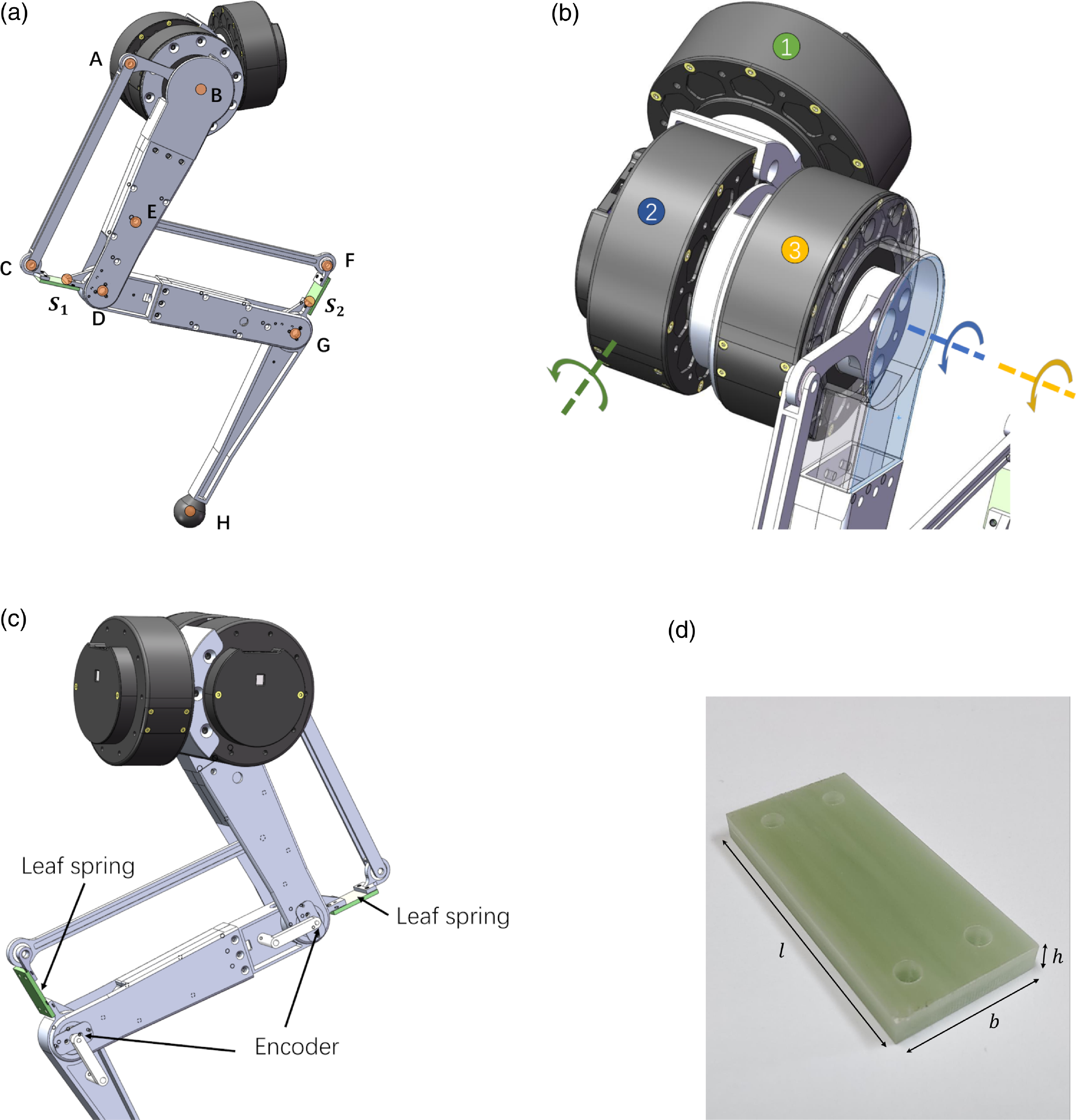
Figure 3. A one-leg robot based on the proposed leg design. (a) Overview of the robot. (b) Detailed view of the motor configuration. (c) Detailed view of the encoder configuration. (d) The epoxy resin leaf spring used in the leg.
For leaf springs, we use off-the-shelf epoxy resin elastic material that used for bows (Fig. 3(d)). After simple cutting and drilling, they can be easily mounted into assigned positions. We alter their width and thickness to adjust the stiffness of leaf springs while keeping the whole leg configuration unchanged. Recall the formula of the stiffness of a cantilever beam:
 \begin{equation} k=\frac{3\textrm{EI}}{l}=\frac{\textrm{E}bh^3}{4l}, \end{equation}
where $\textrm{E}$
denotes the elastic modulus;
$\textrm{E}$
denotes the elastic modulus; $\textrm{I}$
denotes the second moment of area about the neutral axis;
$\textrm{I}$
denotes the second moment of area about the neutral axis; $l$
,
$l$
, $b$
, and
$b$
, and $h$
denote the length, width, and thickness of the leaf spring as shown in Fig. 3(d). This formula indicates that it is enough to alter the stiffness by adjusting width and thickness.
$h$
denote the length, width, and thickness of the leaf spring as shown in Fig. 3(d). This formula indicates that it is enough to alter the stiffness by adjusting width and thickness.
Despite (21), further calibration of the stiffness parameter $k_s$
in (1) and (15) is conducted through experimental-data-based parameter optimization. The optimization problem is constructed as follows:
$k_s$
in (1) and (15) is conducted through experimental-data-based parameter optimization. The optimization problem is constructed as follows:
 \begin{equation} \begin{aligned} \min _{k_{s1},k_{s2},\boldsymbol{{q}}_{\text{off}}} \quad & \sum _{i=1}^{N} w_{x,i}(\,f_{mx,i}-f_{cx,i})^2+w_{y,i}(\,f_{my,i}-f_{cy,i})^2\\ \textrm{s.t.} \quad &[\,f_{cx,i},f_{cy,i}]=g(\boldsymbol{{q}}_{\text{a,i}}-\boldsymbol{{q}}_{\text{off}},k_{s1},k_{s2})\\ &k_{low}\leq k_{s1},k_{s2} \leq k_{upp} \\ \end{aligned} \end{equation}
where $i$
denotes the test index.
$i$
denotes the test index. $f_{mx}$
and
$f_{mx}$
and $f_{my}$
denote the measured foot-end contact forces along the horizontal and vertical axis separately. They are assumed to be “real” values measured from a force plate.
$f_{my}$
denote the measured foot-end contact forces along the horizontal and vertical axis separately. They are assumed to be “real” values measured from a force plate. $f_{cx}$
and
$f_{cx}$
and $f_{cy}$
denote the calculated foot-end contact forces which derived through function
$f_{cy}$
denote the calculated foot-end contact forces which derived through function $g(\cdot )$
according to (17). They are estimated values based on spring deflections.
$g(\cdot )$
according to (17). They are estimated values based on spring deflections. $\boldsymbol{{q}}_{\text{off}}$
denotes offset values for
$\boldsymbol{{q}}_{\text{off}}$
denotes offset values for $\boldsymbol{{q}}_a$
.
$\boldsymbol{{q}}_a$
. $w_{x,i}$
and
$w_{x,i}$
and $w_{y,i}$
are adjustable weights. This optimization problem minimizes the contact force estimation error by optimizing the value of
$w_{y,i}$
are adjustable weights. This optimization problem minimizes the contact force estimation error by optimizing the value of $k_{s1}$
and
$k_{s1}$
and $k_{s2}$
. This is superior to (21) from a practical use perspective. We conduct this optimization procedure based on data acquired from static load tests (Section 4.1). Then, the derived stiffness parameter
$k_{s2}$
. This is superior to (21) from a practical use perspective. We conduct this optimization procedure based on data acquired from static load tests (Section 4.1). Then, the derived stiffness parameter $k_s$
will be used for online contact force estimation according to (17).
$k_s$
will be used for online contact force estimation according to (17).
This robot is designed to work at a nominal leg length of 0.5 m. Based on this leg length, most linkage lengths are decided to guarantee a big enough foot-end workspace. Table I lists their detailed values. The robot weighs about 3 kg, including three motors, about 2.31 kg, and aluminum alloy links, weighing about 0.69 kg. Among all the links, link BD weighs about 0.15 kg, link DG weighs about 0.19 kg, and link GH weighs about 0.14 kg. The encoder weighs about 0.011 kg each. The width of the leaf springs is 20 mm, and the thickness is 3 mm. Moreover, the selected motors have a rated torque of 12 Nm, rated speed of 258 rpm, peak torque of 37 Nm, and peak speed of 300 rpm.
Table I. Kinematic parameters of the one-leg robot.

This one-leg robot costs around 2300 US dollars, including 1200 US dollars for three motors and 1000 US dollars for manufacturing all the links.
3. Control algorithm for periodic hopping
We use a touch-down-event-based control algorithm to achieve periodic hopping for the one-leg robot. For a more apparent revelation of the elasticity of the robot, all motors are controlled in the high-gain feedback position control mode. The hopping motions are realized through the vertical position control of the foot end.
Figure 4 illustrates the overall controller structure. The foot-end trajectory generator receives the user control command and the touch-down event (TD event) to generate leg stretch and contract motion. Its output is the 2D foot-end position in the Cartesian space. Specifically, Fig. 5 depicts the output trajectory along y direction. During one hopping period, the generator will shrink the leg within $t_{sk}$
, then hold this position until the touch-down event is detected. Then, the generator will wait for
$t_{sk}$
, then hold this position until the touch-down event is detected. Then, the generator will wait for $t_{tdw}$
and stretch the leg within
$t_{tdw}$
and stretch the leg within $t_{sr}$
and hold the output position for
$t_{sr}$
and hold the output position for $t_{sr\_h}$
long. For trajectory along the x direction, it will be held at a predefined constant value.
$t_{sr\_h}$
long. For trajectory along the x direction, it will be held at a predefined constant value.

Figure 4. Block diagram of the hopping controller.

Figure 5. Y direction output of the foot-end trajectory generator.
The inverse kinematics module receives the desired foot-end position and derives the desired motor angles in joint space. Note that we do not actively control the compression and release of the leaf springs. Thus, their deflections are considered zero in this module. The TD event detector receives the measured motor angles and the measured angles of joints D and G to judge whether the TD event happens. It estimates the contact forces according to (17). The leaf spring deflections are estimated through (18) and (19). The stiffness parameter $k_s$
is derived offline through (22) static load tests. The TD event is recognized as triggered once the contact force along the vertical direction exceeds a predefined threshold.
$k_s$
is derived offline through (22) static load tests. The TD event is recognized as triggered once the contact force along the vertical direction exceeds a predefined threshold.
The control algorithm is deployed on a Raspberry Pi 4B board [22] with a fixed control period of 5 ms. The control environment is based on Simulink Support Package for Raspberry Pi Hardware from MathWorks [23]. We use the CAN bus to establish the communication between the control board and the motors. The baud rate is 1 Mbit/s.
4. Experiments
The experimental platform is shown in Fig. 6. This platform contains a low-friction vertical slider to mount the one-leg robot, a draw-wire sensor for measuring the hip joint height of the robot, and a 6D force plate to measure the contact forces. The draw-wire sensor is connected to the control board via the CAN bus, and the 6D force plate is connected via UDP protocol. The data acquisition period is 5 ms, the same as the control period.

Figure 6. Experimental platform for the one-leg robot.
Note that for the hopping control, only leaf springs’ deflections are needed for successful continuous hopping. Measurement of the draw-wire sensor and the force plate are not required. Video records of the following tests can be found in the supplementary materials.
4.1. Stiffness calibration and contact forces estimation
We calibrate the leaf spring stiffness according to (22). The robot was statically put on the force plate with different payloads and commanded foot-end positions. We chose the interested foot-end test points at $\boldsymbol{{p}}_{\textrm{H,x}}=[{-}0.05, 0, 0.05]$
m,
$\boldsymbol{{p}}_{\textrm{H,x}}=[{-}0.05, 0, 0.05]$
m, $\boldsymbol{{p}}_{\textrm{H,y}}=[{-}0.4, -0.5]$
m, and with payloads of
$\boldsymbol{{p}}_{\textrm{H,y}}=[{-}0.4, -0.5]$
m, and with payloads of $[0, 3, 5]$
kg. Thus, we have 18 test points in total. These points were chosen to cover the predicted motion range and the payload range for the following hopping motions. For the deploying of (22), all
$[0, 3, 5]$
kg. Thus, we have 18 test points in total. These points were chosen to cover the predicted motion range and the payload range for the following hopping motions. For the deploying of (22), all $w_{x,i}$
are set to 50, and all
$w_{x,i}$
are set to 50, and all $w_{y,i}$
are set to 1. The final evaluation of the stiffness for joint
$w_{y,i}$
are set to 1. The final evaluation of the stiffness for joint $\textrm{S}_1$
is 122.85 Nm/rad and for joint
$\textrm{S}_1$
is 122.85 Nm/rad and for joint $\textrm{S}_2$
is 102.78 Nm/rad.
$\textrm{S}_2$
is 102.78 Nm/rad.
Furthermore, we use the above stiffness values to derive the estimated contact forces according to (17) and compare them with those measured by the force plate. As depicted in Fig. 7(a) and (b), for $f_x$
, the maximum estimation error is 2.424 N, the minimum estimation error is 0.125 N, and the average estimation relative error is 217.95%. For
$f_x$
, the maximum estimation error is 2.424 N, the minimum estimation error is 0.125 N, and the average estimation relative error is 217.95%. For $f_y$
, the maximum estimation error is 23.697 N, the minimum estimation error is 0.549 N, and the average estimation relative error is 15.82%. In conclusion, we have a better estimation of the vertical contact forces. Thus, only the estimated vertical contact force is used to detect the touch-down event in the following hopping test.
$f_y$
, the maximum estimation error is 23.697 N, the minimum estimation error is 0.549 N, and the average estimation relative error is 15.82%. In conclusion, we have a better estimation of the vertical contact forces. Thus, only the estimated vertical contact force is used to detect the touch-down event in the following hopping test.

Figure 7. Comparison between estimated and measured contact forces.
4.2. Dropping test
In this test, we command the foot end to hold at a specific position and drop the robot from a certain height. As shown in Fig. 8, the robot was dropped from 0.7 m, bounced since 0.5 s, and finally statically stayed at 0.5 m after 2.5 s. Note that there were oscillations in estimated forces during the flight phases between 0.7–0.9 s and 1.03–1.19 s. The reason is that when the leg leaves the ground, the leaf springs do not have enough damping forces to suppress the oscillation caused by the pull of the gravity of lower links. The same phenomena are also observed in the periodic hopping test.

Figure 8. Hip joint height in the dropping test.
The equivalent or virtual leg stiffness is measured through the oscillation period of the hip joint height after the foot end steadily touches the ground. As shown in Fig. 8, the desired oscillation period should be measured after 1.5 s, and this period is around 0.16 s. This period can also be estimated by evaluating the vertical stiffness through (20) and substituting it into a simple mass-spring harmonic oscillator model. Specifically for this test, according to (20), the equivalent leg stiffness along the vertical direction is 5569 N/m. Given the leg mass is around 3 kg, the oscillation period should be $2\pi \sqrt{m/k}$
, which is 0.146 s. The estimated oscillation period of 0.146 s is close to the measured one of 0.16 s, indicating that the actual leg stiffness fits the predicted one.
$2\pi \sqrt{m/k}$
, which is 0.146 s. The estimated oscillation period of 0.146 s is close to the measured one of 0.16 s, indicating that the actual leg stiffness fits the predicted one.
4.3. Hopping test
In this test, we control the robot to achieve periodic hopping by deploying the algorithm introduced in Section 3. Snapshots of the hopping test are shown in Fig. 9. Specifically, for the parameters defined in Fig. 5, their values are $l_{sr}=0.14$
m,
$l_{sr}=0.14$
m, $t_{sk}=0.3$
s,
$t_{sk}=0.3$
s, $t_{tdw}=0.04$
s,
$t_{tdw}=0.04$
s, $t_{sr}=0.05$
s,
$t_{sr}=0.05$
s, $t_{sr\_h}=0.14$
s, and
$t_{sr\_h}=0.14$
s, and $p_{H,y0}$ $=-0.54$
m. To evaluate the energy efficiency of the proposed leg design, the hopping test was also conducted in the robot where the leaf springs were replaced with rigid aluminum plates. Note that the touch-down event was detected only by the estimated vertical contact forces rather than the force plate measurement. Moreover, as the compliant joints will oscillate during the flight phase (as shown in Fig. 10), we set a high threshold of 70 N for touch-down event detection to avoid misjudgments. The oscillation happens both at the start of the stance phase and the start of the flight phase. In the stance phase, the oscillation decays rapidly. However, for the flight phase, the oscillation sustains until the leg touches the ground. Thus, the oscillation is mainly caused by the drastic changes in the contact forces. As the motors are controlled in a high-stiffness position mode and low-friction ball bearings are used for leg joints, the energy stored in the compliant joint cannot be consumed efficiently, which leads to the phenomena mentioned above.
$=-0.54$
m. To evaluate the energy efficiency of the proposed leg design, the hopping test was also conducted in the robot where the leaf springs were replaced with rigid aluminum plates. Note that the touch-down event was detected only by the estimated vertical contact forces rather than the force plate measurement. Moreover, as the compliant joints will oscillate during the flight phase (as shown in Fig. 10), we set a high threshold of 70 N for touch-down event detection to avoid misjudgments. The oscillation happens both at the start of the stance phase and the start of the flight phase. In the stance phase, the oscillation decays rapidly. However, for the flight phase, the oscillation sustains until the leg touches the ground. Thus, the oscillation is mainly caused by the drastic changes in the contact forces. As the motors are controlled in a high-stiffness position mode and low-friction ball bearings are used for leg joints, the energy stored in the compliant joint cannot be consumed efficiently, which leads to the phenomena mentioned above.
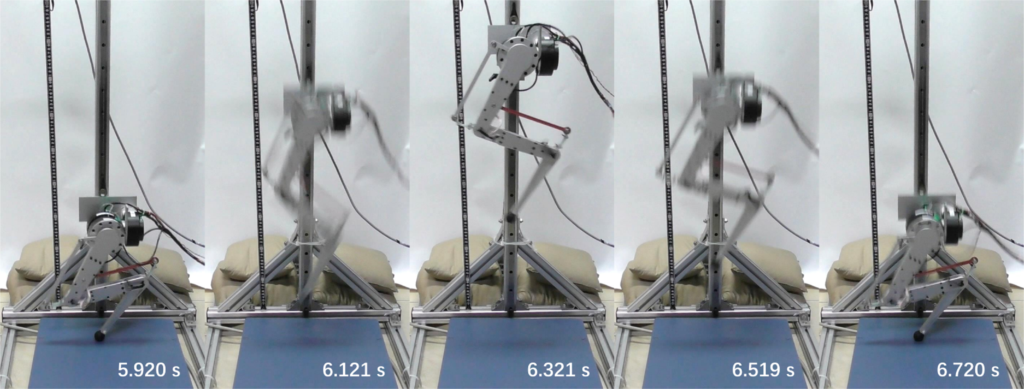
Figure 9. Snapshots of one hopping period.

Figure 10. Comparison between estimated and measured contact forces during periodic hopping.
Figure 11 shows the hip joint height trajectories for the compliant and rigid leg. For the compliant leg, the maximum hip height of one jump slowly increased for four periods and reached a stable value of 0.756 m. The maximum hip height for the rigid leg remained the same since the first period. No increment process has been observed, and its stable maximum hip height value is 0.718 m.

Figure 11. Hip joint height record in hopping tests for compliant and rigid legs.
Figure 12 gives a clearer view of how the maximum hip joint height changes during one hopping test. In this study, one hopping test includes 11 jumps. We measured the maximum hip joint height of each jump and plotted them concerning the time when this height was reached. Data of the compliant leg test 1 and the rigid leg test correspond to the ones that are used in Fig. 11. Compliant leg test 2 shares the same experimental conditions of compliant leg test 1. It is added to illustrate the repeatability of the hopping test. As shown by Fig. 12, the maximum hip joint height of the compliant leg slowly increases while the one of the rigid leg does not. It indicates that the leaf springs store and release the impact energy and increase the energy efficiency.

Figure 12. Change of maximum hip joint height in hopping tests.
To get a quantitative description of the energy efficiency, we define jump height as the difference between the stable maximum hip joint height and the hip joint height when the robot leaves off the ground. In the above tests, the robot leaves the ground when the hip joint height exceeds 0.54 m, which is the value of $p_{H,y0}$
. Thus, the jump height for the compliant leg test 1 is 0.2161 m, for the compliant leg test 2 is 0.21607 m, and for the rigid leg test is 0.1778 m. Thus, jump height is increased by nearly 20% after the leaf springs are deployed and tested under the conditions mentioned above described at the beginning of this section. This indicates the energy efficiency of the proposed leg design.
$p_{H,y0}$
. Thus, the jump height for the compliant leg test 1 is 0.2161 m, for the compliant leg test 2 is 0.21607 m, and for the rigid leg test is 0.1778 m. Thus, jump height is increased by nearly 20% after the leaf springs are deployed and tested under the conditions mentioned above described at the beginning of this section. This indicates the energy efficiency of the proposed leg design.
5. Discussion and conclusion
This paper presents a compliant leg design that combines the pantograph structure with leaf springs. This design has two benefits: (1) Compared with coil springs, leaf springs are easier to deploy and adjust their stiffness through simple cutting, and (2) The configuration of two unparalleled leaf springs allows for thoroughly estimating the 2-DoF contact forces. As validated by the one-leg robot, the mechanism owes predicted elasticity and can estimate the contact forces with little time delay. As the hopping test indicates, the vertical contact force estimation is reasonably good for touch-down event detection. However, estimation errors still exist, and after the leg leaves the ground, there would be oscillations around the compliant joints.
A sophisticated calibration for the motor offset angles, and the mechanism kinematics parameters could help better estimate contact force. Considering the spring deflections for our robot are usually around 1.5–6 degrees, such small angles could easily be disturbed by the error of motor offset angles or kinematics parameters. Sleeve bearings could be used at passive joints to increase damping forces for avoiding oscillations around the compliant joints. Motors controlled in low-stiffness position mode or torque-controlled mode will also help to adsorb the oscillation.
Author contributions
Boxing Wang and Lihao Jia conceived and designed the study. Boxing Wang, Kunting Zhang, and Xueyan Ma conducted algorithm design, experiment design, data gathering, and analyses. Boxing Wang wrote the article.
Financial support
This work was supported by the Natural Science Foundation of China (Grant No. 62003340).
Competing interests
The authors declare no competing interests exist.
Ethical approval
Not applicable.
Supplementary material
To view supplementary material for this article, please visit https://doi.org/10.1017/S0263574723001443


