


1 Introduction
Humans show the remarkable skill to reason in terms of counterfactuals. This means we reason about how events would unfold under different circumstances without actually experiencing all these different realities. For instance, we make judgments like: “If I had taken a bus earlier, I would have arrived on time.” without actually experiencing the alternative reality in which we took the bus earlier. As this capability lies at the basis of making sense of the past, planning courses of actions, making emotional and social judgments as well as adapting our behavior, one also wants an artificial intelligence to reason counterfactually (Hoeck Reference Hoeck2015).
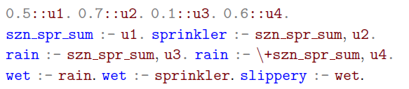
Here, we focus on the counterfactual reasoning with the semantics provided by Pearl (Reference Pearl2000). Our aim is to establish this kind of reasoning in the ProbLog language of De Raedt et al. (Reference De Raedt, Kimmig and Toivonen2007). To illustrate this issue, we introduce a version of the sprinkler example from Pearl (Reference Pearl2000), Section 1.4.
It is spring or summer, written $szn\_spr\_sum$
, with a probability of
$szn\_spr\_sum$
, with a probability of $\pi_1 := 0.5$
. Consider a road, which passes along a field with a sprinkler on it. In spring or summer, the sprinkler is on, written sprinkler, with probability
$\pi_1 := 0.5$
. Consider a road, which passes along a field with a sprinkler on it. In spring or summer, the sprinkler is on, written sprinkler, with probability $\pi_2 := 0.7$
. Moreover, it rains, denoted by rain, with probability
$\pi_2 := 0.7$
. Moreover, it rains, denoted by rain, with probability ${\pi_3 := 0.1}$
in spring or summer and with probability
${\pi_3 := 0.1}$
in spring or summer and with probability $\pi_4 := 0.6$
in fall or winter. If it rains or the sprinkler is on, the pavement of the road gets wet, denoted by wet. When the pavement is wet, the road is slippery, denoted by slippery. Under the usual reading of ProbLog programs, one would model the situation above with the following program
$\pi_4 := 0.6$
in fall or winter. If it rains or the sprinkler is on, the pavement of the road gets wet, denoted by wet. When the pavement is wet, the road is slippery, denoted by slippery. Under the usual reading of ProbLog programs, one would model the situation above with the following program $\textbf{P}$
:
$\textbf{P}$
:
To construct a semantics for the program $\textbf{P,}$
we generate mutually independent Boolean random variables u1-u4 with
$\textbf{P,}$
we generate mutually independent Boolean random variables u1-u4 with $\pi(ui) = \pi_i$
for all
$\pi(ui) = \pi_i$
for all $1 \leq i \leq 4$
. The meaning of the program
$1 \leq i \leq 4$
. The meaning of the program $\textbf{P}$
is then given by the following system of equations:
$\textbf{P}$
is then given by the following system of equations:

Finally, assume we observe that the sprinkler is on and that the road is slippery. What is the probability of the road being slippery if the sprinkler were switched off?
Since we observe that the sprinkler is on, we conclude that it is spring or summer. However, if the sprinkler is off, the only possibility for the road to be slippery is given by rain. Hence, we obtain a probability of $0.1$
for the road to be slippery if the sprinkler were off.
$0.1$
for the road to be slippery if the sprinkler were off.
In this work, we automate this kind of reasoning. However, to the best of our knowledge, current probabilistic logic programming systems cannot evaluate counterfactual queries.While we may ask what the probability of slippery is if we switch the sprinkler off and observe some evidence, we obtain a zero probability for sprinkler after switching the sprinkler off, which renders the corresponding conditional probability meaningless. To circumvent this problem, we adapt the twin network method of Balke and Pearl (Reference Balke and Pearl1994) from causal models to probabilistic logic programming, with a proof of correctness. Notably, this reduces counterfactual reasoning to marginal inference over a modified program. Hence, we can immediately make use of the established efficient inference engines to accomplish our goal.
We also check that our approach is consistent with the counterfactual reasoning for logic programs with annotated disjunctions or LPAD-programs (Vennekens et al. Reference Vennekens, Verbaeten and Bruynooghe2004), which was presented by Vennekens et al. (Reference Vennekens, Bruynooghe and Denecker2010). In this way, we fill the gap of showing that the causal reasoning for LPAD-programs of Vennekens et al. (Reference Vennekens, Denecker and Bruynooghe2009) is indeed consistent with Pearl’s theory of causality and we establish the expressive equivalence of ProbLog and LPAD regarding counterfactual reasoning.
Apart from our theoretical contributions, we provide a full implementation by making use of the aspmc library (Eiter et al. Reference Eiter, Hecher and Kiesel2021). Additionally, we investigate the scalability of the two main approaches used for efficient inference, with respect to program size and structural complexity, as well as the influence of evidence and interventions on performance.
2 Preliminaries
Here, we recall the theory of counterfactual reasoning from Pearl (Reference Pearl2000) before we introduce the ProbLog language of De Raedt et al. (Reference De Raedt, Kimmig and Toivonen2007) in which we would like to process counterfactual queries.
2.1 Pearl’s formal theory of counterfactual reasoning
The starting point of a formal theory of counterfactual reasoning is the introduction of a model that is capable of answering the intended queries. To this aim, we recall the definition of a functional causal model from Pearl (Reference Pearl2000), Sections 1.4.1 and 7 respectively:
Definition 1 (Causal Model)
A functional causal model or causal model $\mathcal{M}$
on a set of variables
$\mathcal{M}$
on a set of variables $\textbf{V}$
is a system of equations, which consists of one equation of the form
$\textbf{V}$
is a system of equations, which consists of one equation of the form $X := f_X (\textrm{pa}(X),\textrm{error}(X))$
for each variable
$X := f_X (\textrm{pa}(X),\textrm{error}(X))$
for each variable $X \in \textbf{V}$
. Here, the parents
$X \in \textbf{V}$
. Here, the parents $\textrm{pa}(X) \subseteq \textbf{V}$
of X form a subset of the set of variables
$\textrm{pa}(X) \subseteq \textbf{V}$
of X form a subset of the set of variables $\textbf{V}$
, the error term
$\textbf{V}$
, the error term $\textrm{error}(X)$
of X is a tuple of random variables, and
$\textrm{error}(X)$
of X is a tuple of random variables, and $f_X$
is a function defining X in terms of the parents
$f_X$
is a function defining X in terms of the parents $\textrm{pa}(X)$
and the error term
$\textrm{pa}(X)$
and the error term $\textrm{error} (X)$
of X.
$\textrm{error} (X)$
of X.
Fortunately, causal models do not only support queries about conditional and unconditional probabilities but also queries about the effect of external interventions. Assume we are given a subset of variables $\textbf{X} := \{ X_1 , ... , X_k \} \subseteq \textbf{V}$
together with a vector of possible values
$\textbf{X} := \{ X_1 , ... , X_k \} \subseteq \textbf{V}$
together with a vector of possible values $\textbf{x} := (x_1,...,x_k)$
for the variables in
$\textbf{x} := (x_1,...,x_k)$
for the variables in $\textbf{X}$
. In order to model the effect of setting the variables in
$\textbf{X}$
. In order to model the effect of setting the variables in $\textbf{X}$
to the values specified by
$\textbf{X}$
to the values specified by $\textbf{x}$
, we simply replace the equations for
$\textbf{x}$
, we simply replace the equations for $X_i$
in
$X_i$
in $\mathcal{M}$
by
$\mathcal{M}$
by $X_i := x_i$
for all
$X_i := x_i$
for all $1 \leq i \leq k$
.
$1 \leq i \leq k$
.
To guarantee that the causal models $\mathcal{M}$
and
$\mathcal{M}$
and $\mathcal{M}^{\textrm{do}(\textbf{X} := \textbf{x})}$
yield well-defined distributions
$\mathcal{M}^{\textrm{do}(\textbf{X} := \textbf{x})}$
yield well-defined distributions $\pi_{\mathcal{M}}(\_)$
and
$\pi_{\mathcal{M}}(\_)$
and $\pi_{\mathcal{M}}(\_ \vert \textrm{do} (\textbf{X} := \textbf{x})),$
we explicitly assert that the systems of equations
$\pi_{\mathcal{M}}(\_ \vert \textrm{do} (\textbf{X} := \textbf{x})),$
we explicitly assert that the systems of equations $\mathcal{M}$
and
$\mathcal{M}$
and $\mathcal{M}^{\textrm{do}(\textbf{X} := \textbf{x})}$
have a unique solution for every tuple
$\mathcal{M}^{\textrm{do}(\textbf{X} := \textbf{x})}$
have a unique solution for every tuple $\textbf{e}$
of possible values for the error terms
$\textbf{e}$
of possible values for the error terms $\textrm{error}(X)$
,
$\textrm{error}(X)$
, $X \in \textbf{V}$
and for every intervention
$X \in \textbf{V}$
and for every intervention $\textbf{X} := \textbf{x}$
.
$\textbf{X} := \textbf{x}$
.
Example 1 The system of equations (1) from Section 1 forms a (functional) causal model on the set of variables $\textbf{V} := \{ szn\_spr\_sum, rain , sprinkler, wet, slippery \}$
if we define
$\textbf{V} := \{ szn\_spr\_sum, rain , sprinkler, wet, slippery \}$
if we define $\textrm{error} (szn\_spr\_sum):= u1$
,
$\textrm{error} (szn\_spr\_sum):= u1$
, $\textrm{error} (sprinkler) := u2$
and
$\textrm{error} (sprinkler) := u2$
and $\textrm{error}(rain) := (u3, u4)$
. To predict the effect of switching the sprinkler on, we simply replace the equation for sprinkler by
$\textrm{error}(rain) := (u3, u4)$
. To predict the effect of switching the sprinkler on, we simply replace the equation for sprinkler by $sprinkler := True$
.
$sprinkler := True$
.
Finally, let $\textbf{E}, \textbf{X} \subseteq \textbf{V}$
be two subset of our set of variables
$\textbf{E}, \textbf{X} \subseteq \textbf{V}$
be two subset of our set of variables $\textbf{V}$
. Now suppose we observe the evidence that
$\textbf{V}$
. Now suppose we observe the evidence that $\textbf{E} = \textbf{e}$
and ask ourselves what would have been happened if we had set
$\textbf{E} = \textbf{e}$
and ask ourselves what would have been happened if we had set $\textbf{X} := \textbf{x}$
. Note that in general
$\textbf{X} := \textbf{x}$
. Note that in general $\textbf{X} = \textbf{x}$
and
$\textbf{X} = \textbf{x}$
and $\textbf{E} = \textbf{e}$
contradict each other. In this case, we talk about a counterfactual query.
$\textbf{E} = \textbf{e}$
contradict each other. In this case, we talk about a counterfactual query.
Example 2 Reconsider the query ${\pi (slippery \vert slippery, sprinkler, \textrm{do} (\neg sprinkler))}$
in the introduction, that is in the causal model (1) we observe the sprinkler to be on and the road to be slippery while asking for the probability of the road to be slippery if the sprinkler were off. This is a counterfactual query as our evidence
${\pi (slippery \vert slippery, sprinkler, \textrm{do} (\neg sprinkler))}$
in the introduction, that is in the causal model (1) we observe the sprinkler to be on and the road to be slippery while asking for the probability of the road to be slippery if the sprinkler were off. This is a counterfactual query as our evidence $\{ sprinkler, slippery \}$
contradicts our intervention
$\{ sprinkler, slippery \}$
contradicts our intervention $\textrm{do} (\neg sprinkler)$
.
$\textrm{do} (\neg sprinkler)$
.
To answer this query based on a causal model $\mathcal{M}$
on
$\mathcal{M}$
on $\textbf{V,}$
we proceed in three steps: In the abduction step, we adjust the distribution of our error terms by replacing the distribution
$\textbf{V,}$
we proceed in three steps: In the abduction step, we adjust the distribution of our error terms by replacing the distribution $\pi_{\mathcal{M}}(\textrm{error}(V))$
with the conditional distribution
$\pi_{\mathcal{M}}(\textrm{error}(V))$
with the conditional distribution $\pi_{\mathcal{M}}(\textrm{error}(V) \vert \textbf{E} = \textbf{e})$
for all variables
$\pi_{\mathcal{M}}(\textrm{error}(V) \vert \textbf{E} = \textbf{e})$
for all variables $V \in \textbf{V}$
. Next, in the action step we intervene in the resulting model according to
$V \in \textbf{V}$
. Next, in the action step we intervene in the resulting model according to $\textbf{X} := \textbf{x}$
. Finally, we are able to compute the desired probabilities
$\textbf{X} := \textbf{x}$
. Finally, we are able to compute the desired probabilities $\pi_{\mathcal{M}}(\_ \vert \textbf{E} = \textbf{e}, \textrm{do} (\textbf{X} := \textbf{x}))$
from the modified model in the prediction step (Pearl Reference Pearl2000, Section 1.4.4). For an illustration of the treatment of counterfactuals, we refer to the introduction.
$\pi_{\mathcal{M}}(\_ \vert \textbf{E} = \textbf{e}, \textrm{do} (\textbf{X} := \textbf{x}))$
from the modified model in the prediction step (Pearl Reference Pearl2000, Section 1.4.4). For an illustration of the treatment of counterfactuals, we refer to the introduction.
To avoid storing the joint distribution $\pi_{\mathcal{M}}(\textrm{error}(V) \vert \textbf{E} = \textbf{e})$
for
$\pi_{\mathcal{M}}(\textrm{error}(V) \vert \textbf{E} = \textbf{e})$
for $V \in \textbf{V,}$
Balke and Pearl (Reference Balke and Pearl1994) developed the twin network method. They first copy the set of variables
$V \in \textbf{V,}$
Balke and Pearl (Reference Balke and Pearl1994) developed the twin network method. They first copy the set of variables $\textbf{V}$
to a set
$\textbf{V}$
to a set $\textbf{V}^{\ast}$
. Further, they build a new causal model
$\textbf{V}^{\ast}$
. Further, they build a new causal model $\mathcal{M}^{K}$
on the variables
$\mathcal{M}^{K}$
on the variables $\textbf{V} \cup \textbf{V}^{\ast}$
by setting
$\textbf{V} \cup \textbf{V}^{\ast}$
by setting
 \begin{align*}V :=\begin{cases}f_X (\textrm{pa}(X), \textrm{error}(X)), & \text{if} V=X \in \textbf{V} \\f_X (\textrm{pa}(X)^{\ast}, \textrm{error}(X)), & \text{if} V=X^{\ast} \in \textbf{V}^{\ast}\end{cases}.\end{align*}
for every $V \in \textbf{V} \cup \textbf{V}^{\ast}$
, where
$V \in \textbf{V} \cup \textbf{V}^{\ast}$
, where $\textrm{pa}(X)^{\ast} := \{ X^{\ast} \vert X \in \textrm{pa}(X) \}$
. Further, they intervene according to
$\textrm{pa}(X)^{\ast} := \{ X^{\ast} \vert X \in \textrm{pa}(X) \}$
. Further, they intervene according to ${\textbf{X}^{\ast} := \textbf{x}}$
to obtain the model
${\textbf{X}^{\ast} := \textbf{x}}$
to obtain the model $\mathcal{M}^{K, \textrm{do}(\textbf{X}^{\ast} := \textbf{x})}$
. Finally, one expects that
$\mathcal{M}^{K, \textrm{do}(\textbf{X}^{\ast} := \textbf{x})}$
. Finally, one expects that
 \begin{align*}\pi_{\mathcal{M}}(\_ \vert \textbf{E} = \textbf{e}, \textrm{do} (\textbf{X} := \textbf{x})) =\pi_{\mathcal{M}^{K, \textrm{do}(\textbf{X}^{\ast} := \textbf{x})}}(\_^{\ast} \vert \textbf{E} = \textbf{e}).\end{align*}
In Example 8, we demonstrate the twin network method for the ProbLog program $\textbf{P}$
and the counterfactual query of the introduction.
$\textbf{P}$
and the counterfactual query of the introduction.
2.2 The ProbLog language
We proceed by recalling the ProbLog language from De Raedt et al. (Reference De Raedt, Kimmig and Toivonen2007). As the semantics of non-ground ProbLog programs is usually defined by grounding, we will restrict ourselves to the propositional case, that is we construct our programs from a propositional alphabet $\mathfrak{P}$
:
$\mathfrak{P}$
:
Definition 2 (propositional alphabet)
A propositional alphabet $\mathfrak{P}$
is a finite set of propositions together with a subset
$\mathfrak{P}$
is a finite set of propositions together with a subset $\mathfrak{E}(\mathfrak{P}) \subseteq \mathfrak{P}$
of external propositions. Further, we call
$\mathfrak{E}(\mathfrak{P}) \subseteq \mathfrak{P}$
of external propositions. Further, we call $\mathfrak{I}(\mathfrak{P}) = \mathfrak{P} \setminus \mathfrak{E} (\mathfrak{P}) $
the set of internal propositions.
$\mathfrak{I}(\mathfrak{P}) = \mathfrak{P} \setminus \mathfrak{E} (\mathfrak{P}) $
the set of internal propositions.
Example 3 To build the ProbLog program $\textbf{P}$
in Section 1, we need the alphabet
$\textbf{P}$
in Section 1, we need the alphabet $\mathfrak{P}$
consisting of the internal propositions
$\mathfrak{P}$
consisting of the internal propositions $\mathfrak{I} (\mathfrak{P}) := \{ szn\_spr\_sum, sprinkler, rain, wet, slippery\}$
and the external propositions
$\mathfrak{I} (\mathfrak{P}) := \{ szn\_spr\_sum, sprinkler, rain, wet, slippery\}$
and the external propositions ${\mathfrak{E} (\mathfrak{P}) := \{ u1, u2, u3, u4 \}}.$
From propositional alphabets, we build literals, clauses, and random facts, where random facts are used to specify the probabilities in our model. To proceed, let us fix a propositional alphabet $\mathfrak{P}$
.
$\mathfrak{P}$
.
Definition 3 (Literal, Clause, and Random Fact)
A literal l is an expression p or $\neg p$
for a proposition
$\neg p$
for a proposition $p \in \mathfrak{P}$
. We call l a positive literal if it is of the form p and a negative literal if it is of the form
$p \in \mathfrak{P}$
. We call l a positive literal if it is of the form p and a negative literal if it is of the form $\neg p$
. A clause LC is an expression of the form
$\neg p$
. A clause LC is an expression of the form $h \leftarrow b_1,...,b_n$
, where
$h \leftarrow b_1,...,b_n$
, where $\textrm{head} (LC) := h \in \mathfrak{I}(\mathfrak{P})$
is an internal proposition and where
$\textrm{head} (LC) := h \in \mathfrak{I}(\mathfrak{P})$
is an internal proposition and where $\textrm{body} (LC) := \{ b_1, ..., b_n \}$
is a finite set of literals. A random fact RF is an expression of the form
$\textrm{body} (LC) := \{ b_1, ..., b_n \}$
is a finite set of literals. A random fact RF is an expression of the form $\pi(RF) :: u(RF)$
, where
$\pi(RF) :: u(RF)$
, where $u(RF) \in \mathfrak{E}(\mathfrak{P})$
is an external proposition and where
$u(RF) \in \mathfrak{E}(\mathfrak{P})$
is an external proposition and where $\pi (RF) \in [0,1]$
is the probability of u(RF).
$\pi (RF) \in [0,1]$
is the probability of u(RF).
Example 4 In Example 3, we have that $szn\_spr\_sum$
is a positive literal, whereas
$szn\_spr\_sum$
is a positive literal, whereas $\neg szn\_spr\_sum$
is a negative literal. Further,
$\neg szn\_spr\_sum$
is a negative literal. Further, $rain \leftarrow \neg szn\_spr\_sum, u4$
is a clause and
$rain \leftarrow \neg szn\_spr\_sum, u4$
is a clause and $0.6 :: u4$
is a random fact.
$0.6 :: u4$
is a random fact.
Next, we give the definition of logic programs and ProbLog programs:
Definition 4 (Logic Program and ProbLog Program)
A logic program is a finite set of clauses. Further, a ProbLog program $\textbf{P}$
is given by a logic program
$\textbf{P}$
is given by a logic program $\textrm{LP} (\textbf{P})$
and a set
$\textrm{LP} (\textbf{P})$
and a set $\textrm{Facts} (\textbf{P})$
, which consists of a unique random fact for every external proposition. We call
$\textrm{Facts} (\textbf{P})$
, which consists of a unique random fact for every external proposition. We call $\textrm{LP} (\textbf{P})$
the underlying logic program of
$\textrm{LP} (\textbf{P})$
the underlying logic program of $\textbf{P}$
.
$\textbf{P}$
.
To reflect the closed world assumption, we omit random facts of the form $0::u$
in the set
$0::u$
in the set $\textrm{Facts} (\textbf{P})$
.
$\textrm{Facts} (\textbf{P})$
.
Example 5 The program $\textbf{P}$
from the introduction is a ProbLog program. We obtain the corresponding underlying logic program
$\textbf{P}$
from the introduction is a ProbLog program. We obtain the corresponding underlying logic program $\textrm{LP} (\textbf{P})$
by erasing all random facts of the form
$\textrm{LP} (\textbf{P})$
by erasing all random facts of the form $\_ :: ui$
from
$\_ :: ui$
from $\textbf{P}$
.
$\textbf{P}$
.
For a set of propositions, $\mathfrak{Q} \subseteq \mathfrak{P}$
a
$\mathfrak{Q} \subseteq \mathfrak{P}$
a $\mathfrak{Q}$
-structure is a function
$\mathfrak{Q}$
-structure is a function $\mathcal{M} :\mathfrak{Q} \rightarrow \{ True , False \}, p \mapsto p^{\mathcal{M}}$
. Whether a formula
$\mathcal{M} :\mathfrak{Q} \rightarrow \{ True , False \}, p \mapsto p^{\mathcal{M}}$
. Whether a formula $\phi$
is satisfied by a
$\phi$
is satisfied by a $\mathfrak{Q}$
-structure
$\mathfrak{Q}$
-structure $\mathcal{M}$
, written
$\mathcal{M}$
, written $\mathcal{M}\models \phi$
, is defined as usual in propositional logic. As the semantics of a logic program
$\mathcal{M}\models \phi$
, is defined as usual in propositional logic. As the semantics of a logic program $\textbf{P}$
with stratified negation, we take the assignment
$\textbf{P}$
with stratified negation, we take the assignment $\mathcal{E} \mapsto \mathcal{M} (\mathcal{E}, \textbf{P})$
that relates each
$\mathcal{E} \mapsto \mathcal{M} (\mathcal{E}, \textbf{P})$
that relates each $\mathfrak{E}$
-structure
$\mathfrak{E}$
-structure $\mathcal{E}$
with the minimal model
$\mathcal{E}$
with the minimal model $\mathcal{M} (\mathcal{E}, \textbf{P})$
of the program
$\mathcal{M} (\mathcal{E}, \textbf{P})$
of the program $\textbf{P} \cup \mathcal{E}$
.
$\textbf{P} \cup \mathcal{E}$
.
3 Counterfactual reasoning: Intervening and observing simultaneously
We return to the objective of this paper, establishing Pearl’s treatment of counterfactual queries in ProbLog. As a first step, we introduce a new semantics for ProbLog programs in terms of causal models.
Definition 5 (FCM-semantics)
For a ProbLog program $\textbf{P,}$
the functional causal model semantics or FCM-semantics is the system of equations that is given by
$\textbf{P,}$
the functional causal model semantics or FCM-semantics is the system of equations that is given by
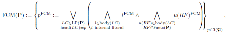 \begin{align*}\textrm{FCM} (\textbf{P}) :=\left\{\!p^{\textrm{FCM}} := \bigvee_{\substack{LC \in \textrm{LP} (\textbf{P}) \\ \textrm{head}(LC) = p}}\!\left(\bigwedge_{\substack{l \in \textrm{body} (LC)\\ l\text{internal literal}}}\!\!\! l^{\textrm{FCM}} \land\!\!\bigwedge_{\substack{u(RF) \in \textrm{body} (LC)\\ RF \in \textrm{Facts} (\textbf{P})}} \!\!\!u(RF)^{\textrm{FCM}}\!\!\right)\!\!\right\}_{p \in \mathfrak{I}(\mathfrak{P})},\end{align*}
where $u(RF)^{\textrm{FCM}}$
are mutually independent Boolean random variables for every random fact
$u(RF)^{\textrm{FCM}}$
are mutually independent Boolean random variables for every random fact $RF \in \textrm{Facts}(\textbf{P})$
that are distributed according to
$RF \in \textrm{Facts}(\textbf{P})$
that are distributed according to $\pi \left[ u(RF)^{\textrm{FCM}} \right] = \pi(RF)$
. Here, an empty disjunction evaluates to False and an empty conjunction evaluates to True.
$\pi \left[ u(RF)^{\textrm{FCM}} \right] = \pi(RF)$
. Here, an empty disjunction evaluates to False and an empty conjunction evaluates to True.
Further, we say that $\textbf{P}$
has unique supported models if
$\textbf{P}$
has unique supported models if $\textrm{FCM} (\textbf{P})$
is a causal model, that is if it possesses a unique solution for every
$\textrm{FCM} (\textbf{P})$
is a causal model, that is if it possesses a unique solution for every $\mathfrak{E}$
-structure
$\mathfrak{E}$
-structure $\mathcal{E}$
and every possible intervention
$\mathcal{E}$
and every possible intervention $\textbf{X} := \textbf{x}$
. In this case, the superscript
$\textbf{X} := \textbf{x}$
. In this case, the superscript $\textrm{FCM}$
indicates that the expressions are interpreted according to the FCM-semantics as random variables rather than predicate symbols. It will be omitted if the context is clear. For a Problog program
$\textrm{FCM}$
indicates that the expressions are interpreted according to the FCM-semantics as random variables rather than predicate symbols. It will be omitted if the context is clear. For a Problog program $\textbf{P}$
with unique supported models, the causal model
$\textbf{P}$
with unique supported models, the causal model $\textrm{FCM} (\textbf{P})$
determines a unique joint distribution
$\textrm{FCM} (\textbf{P})$
determines a unique joint distribution $\pi_{\textbf{P}}^{\textrm{FCM}}$
on
$\pi_{\textbf{P}}^{\textrm{FCM}}$
on $\mathfrak{P}$
. Finally, for a
$\mathfrak{P}$
. Finally, for a $\mathfrak{P}$
-formula
$\mathfrak{P}$
-formula $\phi$
we define the probability to be true by
$\phi$
we define the probability to be true by
 \begin{align*}\pi_{\textbf{P}}^{\textrm{FCM}}(\phi) := \sum_{\substack{\mathcal{M} \mathfrak{P}\text{-structure} \\ \mathcal{M} \models \phi}} \pi_{\textbf{P}}^{\textrm{FCM}}(\mathcal{M}) =\sum_{\substack{\mathcal{E} \mathfrak{E}\text{-structure} \\ \mathcal{M}(\mathcal{E}, \textbf{P}) \models \phi}} \pi_{\textbf{P}}^{\textrm{FCM}}(\mathcal{E}) .\end{align*}
Example 6 As intended in the introduction, the causal model (1) yields the FCM-semantics of the program $\textbf{P}$
. Now let us calculate the probability
$\textbf{P}$
. Now let us calculate the probability $\pi_{\textbf{P}}^{\textrm{FCM}} (sprinkler)$
that the sprinkler is on.
$\pi_{\textbf{P}}^{\textrm{FCM}} (sprinkler)$
that the sprinkler is on.
 \begin{align*} & \pi_{\textbf{P}}^{\textrm{FCM}} (sprinkler) = \sum_{\substack{\mathcal{M} \mathfrak{P}\text{-structure} \\ \mathcal{M} \models sprinkler}} \pi_{\textbf{P}}^{\textrm{FCM}}(\mathcal{M}) = \sum_{\substack{\mathcal{E} \mathfrak{E}\text{-structure} \\ \mathcal{M}(\mathcal{E}, \textbf{P}) \models sprinker}} \pi_{\textbf{P}}^{\textrm{FCM}}(\mathcal{E}) = \\& = \pi (u1,u2,u3,u4)+ \pi (u1,u2,\neg u3,u4)+ \pi (u1,u2,u3, \neg u4)\\ &\qquad + \pi (u1,u2,\neg u3, \neg u4) \stackrel{\substack{ui \text{mutually} \\ \text{independent}}}{=} \\& = 0.5 \cdot 0.7 \cdot 0.1 \cdot 0.6+ 0.5 \cdot 0.7 \cdot 0.9 \cdot 0.6+ 0.5 \cdot 0.7 \cdot 0.1 \cdot 0.4 + 0.5 \cdot 0.7 \cdot 0.9 \cdot 0.4 = 0.35\end{align*}
As desired, we obtain that the FCM-semantics consistently generalizes the distribution semantics of Poole (Reference Poole1993) and Sato (Reference Sato1995).
Theorem 1 (Rückschloß and Weitkämper Reference Rückschloß and Weitkämper2022)
Let $\textbf{P}$
be a ProbLog program with unique supported models. The FCM-semantics defines a joint distribution
$\textbf{P}$
be a ProbLog program with unique supported models. The FCM-semantics defines a joint distribution $\pi_{\textbf{P}}^{\textrm{FCM}}$
on
$\pi_{\textbf{P}}^{\textrm{FCM}}$
on $\mathfrak{P}$
, which coincides with the distribution semantics
$\mathfrak{P}$
, which coincides with the distribution semantics $\pi_{\textbf{P}}^{dist}$
.
$\pi_{\textbf{P}}^{dist}$
. $\square$
As intended, our new semantics transfers the query types of functional causal models to the framework of ProbLog. Let $\textbf{P}$
be a ProbLog program with unique supported models. First, we discuss the treatment of external interventions.
$\textbf{P}$
be a ProbLog program with unique supported models. First, we discuss the treatment of external interventions.
Let $\phi$
be a
$\phi$
be a $\mathfrak{P}$
-formula and let
$\mathfrak{P}$
-formula and let $\textbf{X} \subseteq \mathfrak{I}(\mathfrak{P})$
be a subset of internal propositions together with a truth value assignment
$\textbf{X} \subseteq \mathfrak{I}(\mathfrak{P})$
be a subset of internal propositions together with a truth value assignment $\textbf{x}$
. Assume we would like to calculate the probability
$\textbf{x}$
. Assume we would like to calculate the probability $\pi_{\textbf{P}}^{FCM}(\phi \vert \textrm{do} (\textbf{X} := \textbf{x}))$
of
$\pi_{\textbf{P}}^{FCM}(\phi \vert \textrm{do} (\textbf{X} := \textbf{x}))$
of $\phi$
being true after setting the random variables in
$\phi$
being true after setting the random variables in $\textbf{X}^{\textrm{FCM}}$
to the truth values specified by
$\textbf{X}^{\textrm{FCM}}$
to the truth values specified by $\textbf{x}$
. In this case, the Definition 1 and Definition 5 yield the following algorithm:
$\textbf{x}$
. In this case, the Definition 1 and Definition 5 yield the following algorithm:
Procedure 1 (Treatment of External Interventions)
We build a modified program $\textbf{P}^{\textrm{do}(\textbf{X} := \textbf{x})}$
by erasing for every proposition
$\textbf{P}^{\textrm{do}(\textbf{X} := \textbf{x})}$
by erasing for every proposition $h \in \textbf{X}$
each clause
$h \in \textbf{X}$
each clause $LC \in \textrm{LP} (\textbf{P})$
with
$LC \in \textrm{LP} (\textbf{P})$
with $\textrm{head}(LC) = h$
and adding the fact
$\textrm{head}(LC) = h$
and adding the fact $h \leftarrow$
to
$h \leftarrow$
to $\textrm{LP} (\textbf{P})$
if
$\textrm{LP} (\textbf{P})$
if $h^{\textbf{x}} = True$
.
$h^{\textbf{x}} = True$
.
Finally, we query the program $\textbf{P}^{\textrm{do}(\textbf{X} := \textbf{x})}$
for the probability of
$\textbf{P}^{\textrm{do}(\textbf{X} := \textbf{x})}$
for the probability of $\phi$
to obtain the desired probability
$\phi$
to obtain the desired probability $\pi_{\textbf{P}}^{\textrm{FCM}}(\phi \vert \textrm{do} (\textbf{X} := \textbf{x}))$
.
$\pi_{\textbf{P}}^{\textrm{FCM}}(\phi \vert \textrm{do} (\textbf{X} := \textbf{x}))$
.
From the construction of the program $\textbf{P}^{\textrm{do}(\textbf{X} := \textbf{x})}$
in Procedure 1, we derive the following classification of programs with unique supported models.
$\textbf{P}^{\textrm{do}(\textbf{X} := \textbf{x})}$
in Procedure 1, we derive the following classification of programs with unique supported models.
Proposition 2 (Characterization of Programs with Unique Supported Models)
A ProbLog program $\textbf{P}$
has unique supported models if and only if for every
$\textbf{P}$
has unique supported models if and only if for every $\mathfrak{E}$
-structure
$\mathfrak{E}$
-structure $\mathcal{E}$
and for every truth value assignment
$\mathcal{E}$
and for every truth value assignment $\textbf{x}$
on a subset of internal propositions
$\textbf{x}$
on a subset of internal propositions $\textbf{X} \subseteq \mathfrak{I}(\mathfrak{P})$
there exists a unique model
$\textbf{X} \subseteq \mathfrak{I}(\mathfrak{P})$
there exists a unique model $\mathcal{M}\left( \mathcal{E}, \textrm{LP} \left( \textbf{P}^{\textrm{do} (\textbf{X} := \textbf{x})} \right) \right)$
of the logic program
$\mathcal{M}\left( \mathcal{E}, \textrm{LP} \left( \textbf{P}^{\textrm{do} (\textbf{X} := \textbf{x})} \right) \right)$
of the logic program $\textrm{LP} \left( \textbf{P}^{\textrm{do} (\textbf{X} := \textbf{x})} \right) \cup \mathcal{E}$
. In particular, the program
$\textrm{LP} \left( \textbf{P}^{\textrm{do} (\textbf{X} := \textbf{x})} \right) \cup \mathcal{E}$
. In particular, the program $\textbf{P}$
has unique supported model if its underlying logic program
$\textbf{P}$
has unique supported model if its underlying logic program $\textrm{LP} (\textbf{P})$
is acyclic.
$\textrm{LP} (\textbf{P})$
is acyclic. $\square$
Example 7 As the underlying logic program of the ProbLog program $\textbf{P}$
in the introduction is acyclic, we obtain from Proposition 2 that it is a ProbLog program with unique supported models that is its FCM-semantics is well-defined.
$\textbf{P}$
in the introduction is acyclic, we obtain from Proposition 2 that it is a ProbLog program with unique supported models that is its FCM-semantics is well-defined.
However, we do not only want to either observe or intervene. We also want to observe and intervene simultaneously. Let $\textbf{E} \subseteq \mathfrak{I}(\mathfrak{P})$
be another subset of internal propositions together with a truth value assignment
$\textbf{E} \subseteq \mathfrak{I}(\mathfrak{P})$
be another subset of internal propositions together with a truth value assignment $\textbf{e}$
. Now suppose we observe the evidence
$\textbf{e}$
. Now suppose we observe the evidence $\textbf{E}^{\textrm{FCM}} = \textbf{e}$
and we ask ourselves what is the probability
$\textbf{E}^{\textrm{FCM}} = \textbf{e}$
and we ask ourselves what is the probability $\pi_{\textbf{P}}^{\textrm{FCM}} (\phi \vert \textbf{E} = \textbf{e} , \textrm{do} (\textbf{X} := \textbf{x}))$
of the formula
$\pi_{\textbf{P}}^{\textrm{FCM}} (\phi \vert \textbf{E} = \textbf{e} , \textrm{do} (\textbf{X} := \textbf{x}))$
of the formula $\phi$
to hold if we had set
$\phi$
to hold if we had set $\textbf{X}^{\textrm{FCM}} := \textbf{x}$
. Note that again we explicitly allow
$\textbf{X}^{\textrm{FCM}} := \textbf{x}$
. Note that again we explicitly allow $\textbf{e}$
and
$\textbf{e}$
and $\textbf{x}$
to contradict each other. The twin network method of Balke and Pearl (Reference Balke and Pearl1994) yields the following procedure to answer those queries in ProbLog:
$\textbf{x}$
to contradict each other. The twin network method of Balke and Pearl (Reference Balke and Pearl1994) yields the following procedure to answer those queries in ProbLog:
Procedure 2 (Treatment of Counterfactuals)
First, we define two propositional alphabets $\mathfrak{P}^{e}$
to handle the evidence and
$\mathfrak{P}^{e}$
to handle the evidence and $\mathfrak{P}^{i}$
to handle the interventions. In particular, we set
$\mathfrak{P}^{i}$
to handle the interventions. In particular, we set $\mathfrak{E}(\mathfrak{P}^{e}) = \mathfrak{E} ( \mathfrak{P}^{i} ) = \mathfrak{E} (\mathfrak{P})$
and
$\mathfrak{E}(\mathfrak{P}^{e}) = \mathfrak{E} ( \mathfrak{P}^{i} ) = \mathfrak{E} (\mathfrak{P})$
and $\mathfrak{I}(\mathfrak{P}^{e/i}) := \left\{ p^{e/i} \text{ : } p \in \mathfrak{I} (\mathfrak{P}) \right\}$
with
$\mathfrak{I}(\mathfrak{P}^{e/i}) := \left\{ p^{e/i} \text{ : } p \in \mathfrak{I} (\mathfrak{P}) \right\}$
with ${\mathfrak{I}(\mathfrak{P}^{e}) \cap \mathfrak{I}(\mathfrak{P}^{i}) = \emptyset}$
. In this way, we obtain maps
${\mathfrak{I}(\mathfrak{P}^{e}) \cap \mathfrak{I}(\mathfrak{P}^{i}) = \emptyset}$
. In this way, we obtain maps $\_^{e/i} : \mathfrak{P} \rightarrow \mathfrak{P}^{e/i}, p \mapsto\begin{cases}p^{e/i}, & p \in \mathfrak{I} (\mathfrak{P}) \\p , & \text{else}\end{cases}$
that easily generalize to literals, clauses, programs, etc.
$\_^{e/i} : \mathfrak{P} \rightarrow \mathfrak{P}^{e/i}, p \mapsto\begin{cases}p^{e/i}, & p \in \mathfrak{I} (\mathfrak{P}) \\p , & \text{else}\end{cases}$
that easily generalize to literals, clauses, programs, etc.
Further, we define the counterfactual semantics of $\textbf{P}$
by
$\textbf{P}$
by $\textbf{P}^{K} := \textbf{P}^{e} \cup \textbf{P}^{i}$
. Next, we intervene in
$\textbf{P}^{K} := \textbf{P}^{e} \cup \textbf{P}^{i}$
. Next, we intervene in $\textbf{P}^{K}$
according to
$\textbf{P}^{K}$
according to $\textrm{do} ( \textbf{X}^i := \textbf{x} )$
and obtain the program
$\textrm{do} ( \textbf{X}^i := \textbf{x} )$
and obtain the program $\textbf{P}^{K, \textrm{do} (\textbf{X}^i := \textbf{x})}$
of Procedure 1. Finally, we obtain the desired probability
$\textbf{P}^{K, \textrm{do} (\textbf{X}^i := \textbf{x})}$
of Procedure 1. Finally, we obtain the desired probability $\pi_{\textbf{P}}^{FCM} (\phi \vert \textbf{E} = \textbf{e} , \textrm{do} (\textbf{X} := \textbf{x}))$
by querying the program
$\pi_{\textbf{P}}^{FCM} (\phi \vert \textbf{E} = \textbf{e} , \textrm{do} (\textbf{X} := \textbf{x}))$
by querying the program $\textbf{P}^{K, \textrm{do} (\textbf{X}^i := \textbf{x})}$
for the conditional probability
$\textbf{P}^{K, \textrm{do} (\textbf{X}^i := \textbf{x})}$
for the conditional probability $\pi (\phi^i \vert \textbf{E}^e = \textbf{e})$
.
$\pi (\phi^i \vert \textbf{E}^e = \textbf{e})$
.
Example 8 Consider the program $\textbf{P}$
of Example 5 and assume we observe that the sprinkler is on and that it is slippery. To calculate the probability
$\textbf{P}$
of Example 5 and assume we observe that the sprinkler is on and that it is slippery. To calculate the probability $\pi (slippery \vert sprinkler , slippery, \textrm{do} (\neg sprinkler))$
that it is slippery if the sprinkler was off, we need to process the query
$\pi (slippery \vert sprinkler , slippery, \textrm{do} (\neg sprinkler))$
that it is slippery if the sprinkler was off, we need to process the query $\pi (slippery^i \vert slippery^e, sprinkler^e)$
on the following program
$\pi (slippery^i \vert slippery^e, sprinkler^e)$
on the following program $\textbf{P}^{K, \textrm{do} (\neg sprinkler^i)}$
.
$\textbf{P}^{K, \textrm{do} (\neg sprinkler^i)}$
.
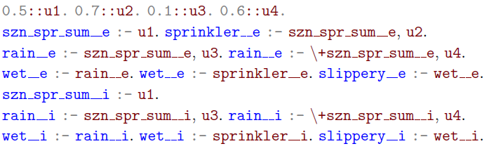
Note that we use the string ${\_\_}$
to refer to the superscript
${\_\_}$
to refer to the superscript $e/i$
.
$e/i$
.
In the Appendix, we prove the following result, stating that a ProbLog program $\textbf{P}$
yields the same answers to counterfactual queries, denoted
$\textbf{P}$
yields the same answers to counterfactual queries, denoted $\pi_{\textbf{P}}^{\textrm{FCM}}(\_ \vert \_)$
, as the causal model
$\pi_{\textbf{P}}^{\textrm{FCM}}(\_ \vert \_)$
, as the causal model $\textrm{FCM} (\textbf{P})$
, denoted
$\textrm{FCM} (\textbf{P})$
, denoted $\pi_{\textrm{FCM} (\textbf{P})} (\_ \vert \_)$
.
$\pi_{\textrm{FCM} (\textbf{P})} (\_ \vert \_)$
.
Theorem 3 (Correctness of our Treatment of Counterfactuals)
Our treatment of counterfactual queries in Procedure 2 is correct that is in the situation of Procedure 2 we obtain that $\pi_{\textbf{P}}^{FCM} (\phi \vert \textbf{E} = \textbf{e} , \textrm{do} (\textbf{X} := \textbf{x}))=\pi_{\textrm{FCM}(\textbf{P})} (\phi \vert \textbf{E} = \textbf{e} , \textrm{do} (\textbf{X} := \textbf{x})).$
4 Relation to CP-logic
Vennekens et al. (Reference Vennekens, Denecker and Bruynooghe2009) establish CP-logic as a causal semantics for the LPAD-programs of Vennekens et al. (Reference Vennekens, Verbaeten and Bruynooghe2004). Further, recall Riguzzi (Reference Riguzzi2020), Section 2.4 to see that each LPAD-program $\textbf{P}$
can be translated to a ProbLog program
$\textbf{P}$
can be translated to a ProbLog program $\textrm{Prob} (\textbf{P})$
such that the distribution semantics is preserved. Analogously, we can read each ProbLog program
$\textrm{Prob} (\textbf{P})$
such that the distribution semantics is preserved. Analogously, we can read each ProbLog program $\textbf{P}$
as an LPAD-Program
$\textbf{P}$
as an LPAD-Program $\textrm{LPAD} (\textbf{P})$
with the same distribution semantics as
$\textrm{LPAD} (\textbf{P})$
with the same distribution semantics as $\textbf{P}$
.
$\textbf{P}$
.
As CP-logic yields a causal semantics, it allows us to answer queries about the effect of external interventions. More generally, Vennekens et al. (Reference Vennekens, Bruynooghe and Denecker2010) even introduce a counterfactual reasoning on the basis of CP-logic. However, to our knowledge this treatment of counterfactuals is neither implemented nor shown to be consistent with the formal theory of causality in Pearl (Reference Pearl2000).
Further, it is a priori unclear whether the expressive equivalence of LPAD and ProbLog programs persists for counterfactual queries. In the Appendix, we compare the treatment of counterfactuals under CP-logic and under the FCM-semantics. This yields the following results.
Theorem 4 (Consistency with CP-Logic – Part 1)
Let $\textbf{P}$
be a propositional LPAD-program such that every selection yields a logic program with unique supported models. Further, let
$\textbf{P}$
be a propositional LPAD-program such that every selection yields a logic program with unique supported models. Further, let $\textbf{X}$
and
$\textbf{X}$
and $\textbf{E}$
be subsets of propositions with truth value assignments, given by the vectors
$\textbf{E}$
be subsets of propositions with truth value assignments, given by the vectors $\textbf{x}$
and
$\textbf{x}$
and $\textbf{e,}$
respectively. Finally, we fix a formula
$\textbf{e,}$
respectively. Finally, we fix a formula $\phi$
and denote by
$\phi$
and denote by $\pi_{\textrm{Prob}(\textbf{P})/\textbf{P}}^{CP/FCM} (\phi \vert \textbf{E} = e, \textrm{do} (\textbf{X} := \textbf{x}))$
the probability that
$\pi_{\textrm{Prob}(\textbf{P})/\textbf{P}}^{CP/FCM} (\phi \vert \textbf{E} = e, \textrm{do} (\textbf{X} := \textbf{x}))$
the probability that $\phi$
is true, given that we observe
$\phi$
is true, given that we observe $\textbf{E} = \textbf{e}$
while we had set
$\textbf{E} = \textbf{e}$
while we had set $\textbf{X} := \textbf{x}$
under CP-logic and the FCM-semantics respectively. In this case, we obtain
$\textbf{X} := \textbf{x}$
under CP-logic and the FCM-semantics respectively. In this case, we obtain $\pi_{\textbf{P}}^{CP} (\phi \vert \textbf{E} = e, \textrm{do} (\textbf{X} := \textbf{x}))=\pi_{\textrm{Prob}(\textbf{P})}^{FCM} (\phi \vert \textbf{E} = e, \textrm{do} (\textbf{X} := \textbf{x})).$
Theorem 5 (Consistency with CP-Logic – Part 2)
If we reconsider the situation of Theorem 4 and assume that $\textbf{P}$
is a ProbLog program with unique supported models, we obtain
$\textbf{P}$
is a ProbLog program with unique supported models, we obtain $\pi_{\textrm{LPAD}(\textbf{P})}^{CP} (\phi \vert \textbf{E} = e, \textrm{do} (\textbf{X} := \textbf{x}))=\pi_{\textbf{P}}^{FCM} (\phi \vert \textbf{E} = e, \textrm{do} (\textbf{X} := \textbf{x})).$
Remark 1 We can also apply Procedure 2 to programs with stratified negation. In this case, the proofs of Theorems 4 and 5 do not need to be modified in order to yield the same statement. However, recalling Definition 1, we see that there is no theory of counterfactual reasoning for those programs. Hence, to us it is not clear how to interpret the results of Procedure 2 for programs that do not possess unique supported models.
In Theorems 4 and 5, we show that under the translations $\textrm{Prob}(\_)$
and
$\textrm{Prob}(\_)$
and $\textrm{LPAD}(\_)$
CP-logic for LPAD-programs is equivalent to our FCM-semantics, which itself by Theorem 3 is consistent with the formal theory of Pearl’s causality. In this way, we fill the gap by showing that the causal reasoning provided for CP-logic is actually correct. Further, Theorems 4 and 5 show that the translations
$\textrm{LPAD}(\_)$
CP-logic for LPAD-programs is equivalent to our FCM-semantics, which itself by Theorem 3 is consistent with the formal theory of Pearl’s causality. In this way, we fill the gap by showing that the causal reasoning provided for CP-logic is actually correct. Further, Theorems 4 and 5 show that the translations $\textrm{Prob}(\_)$
and
$\textrm{Prob}(\_)$
and $\textrm{LPAD} (\_)$
of Riguzzi (Reference Riguzzi2020), Section 2.4 do not only respect the distribution semantics but also are equivalent for more general causal queries.
$\textrm{LPAD} (\_)$
of Riguzzi (Reference Riguzzi2020), Section 2.4 do not only respect the distribution semantics but also are equivalent for more general causal queries.
5 Practical evaluation
We have seen that we can solve counterfactual queries by performing marginal inference over a rewritten probabilistic logic program with evidence. Most of the existing solvers for marginal inference, including ProbLog (Fierens et al. Reference Fierens, den Broeck, Renkens, Shterionov, Gutmann, Thon, Janssens and De Raedt2015), aspmc (Eiter et al. Reference Eiter, Hecher and Kiesel2021), and PITA (Riguzzi and Swift Reference Riguzzi and Swift2011), can handle probabilistic queries with evidence in one way or another. Therefore, our theoretical results also immediately enable the use of these tools for efficient evaluation in practice.
Knowledge Compilation for Evaluation
The currently most successful strategies for marginal inference make use of Knowledge Compilation (KC). They compile the logical theory underlying a probabilistic logic program into a so-called tractable circuit representation, such as binary decision diagrams (BDD), sentential decision diagrams (SDD) (Darwiche Reference Darwiche2011) or smooth deterministic decomposable negation normal forms (sd-DNNF). While the resulting circuits may be much larger (up to exponentially in the worst case) than the original program, they come with the benefit that marginal inference for the original program is possible in polynomial time in their size (Darwiche and Marquis Reference Darwiche and Marquis2002).
When using KC, we can perform compilation either bottom-up or top-down. In bottom-up KC, we compile SDDs representing the truth of internal atoms in terms of only the truth of the external atoms. After combining the SDDs for the queries with the SDDs for the evidence, we can perform marginal inference on the results (Fierens et al. Reference Fierens, den Broeck, Renkens, Shterionov, Gutmann, Thon, Janssens and De Raedt2015).
For top-down KC, we introduce auxiliary variables for internal atoms, translate the program into a CNF, and compile an sd-DNNF for the whole theory. Again, we can perform marginal inference on the result (Eiter et al. Reference Eiter, Hecher and Kiesel2021).
Implementation As the basis of our implementation, we make use of the solver library aspmc. It supports parsing, conversion to CNF and top-down KC including a KC-version of sharpSAT Footnote 1 based on the work of Korhonen and J¨arvisalo (2021). Additionally, we added (i) the program transformation that introduces the duplicate atoms for the evidence part and the query part, and (ii) allowed for counterfactual queries based on it.
Furthermore, to obtain empirical results for bottom-up KC, we use PySDD, Footnote 2 which is a python wrapper around the SDD library of Choi and Darwiche (Reference Choi and Darwiche2013). This is also the library that ProbLog uses for bottom-up KC to SDDs.
6 Empirical evaluation
Here, we consider the scaling of evaluating counterfactual queries by using our translation to marginal inference. This can depend on (i) the number of atoms and rules in the program, (ii) the complexity of the program structure, and (iii) the number and type of interventions and evidence.
We investigate the influence of these parameters on both the bottom-up and top-down KC. Although top-down KC as in aspmc can be faster (Eiter et al. Reference Eiter, Hecher and Kiesel2021) on usual marginal queries, results for bottom-up KC are relevant nevertheless since it is heavily used in ProbLog and PITA.
Furthermore, it is a priori not clear that the performance of these approaches on usual instances of marginal inference translates to the marginal queries obtained by our translation. Namely, they exhibit a lot of symmetries as we essentially duplicate the program as a first step of the translation. Thus, the scaling of both approaches and a comparison thereof is of interest.
6.1 Questions and hypotheses
The first question we consider addresses the scalability of the bottom-up and top-down approaches in terms of the size of the program and the complexity of the program structure.
Q1. Size and Structure: What size and complexity of counterfactual query instances can be solved with bottom-up or top-down compilation?
Here, we expect similar scaling as for marginal inference, since evaluating one query is equivalent to performing marginal inference once. While we duplicate the atoms that occur in the instance, thus increasing the hardness, we can also make use of the evidence, which can decrease the hardness, since we can discard models that do not satisfy the evidence.
Since top-down compilation outperformed bottom-up compilation on marginal inference instances in related work (Eiter et al. Reference Eiter, Hecher and Kiesel2021), we expect that the top-down approach scales better than the bottom-up approach.
Second, we are interested in the influence that the number of intervention and evidence atoms has, in addition to whether it is a positive or negative intervention/evidence atom.
Q2. Evidence and Interventions: How does the number and type of evidence and intervention atoms influence the performance?
We expect that evidence and interventions can lead to simplifications for the program. However, it is not clear whether this is the case in general, whether it only depends on the number of evidence/intervention atoms, and whether there is a difference between negative and positive evidence/intervention atoms.
6.2 Setup
We describe how we aim to answer the questions posed in the previous subsection.
Benchmark Instances As instances, we consider acyclic-directed graphs G with distinguished start and goal nodes s and g. Here, we use the following probabilistic logic program to model the probability of reaching a vertex in G:

Here,
![]() refers to the number of outgoing arcs of X in G, and
refers to the number of outgoing arcs of X in G, and
![]() refer to its direct descendants. We obtain the final program by replacing the variables X,Y with constants corresponding to the vertices of G.
refer to its direct descendants. We obtain the final program by replacing the variables X,Y with constants corresponding to the vertices of G.
This program models that we reach (denoted by
![]() ) the starting vertex s and, at each vertex v that we reach, decide uniformly at random which outgoing arc we include in our path (denoted by
) the starting vertex s and, at each vertex v that we reach, decide uniformly at random which outgoing arc we include in our path (denoted by
![]() ). If we include the arc (v,w), then we reach the vertex w. However, we only include an outgoing arc, if we do not get trapped (denoted by
). If we include the arc (v,w), then we reach the vertex w. However, we only include an outgoing arc, if we do not get trapped (denoted by
![]() ) at v.
) at v.
This allows us to pose counterfactual queries regarding the probability of reaching the goal vertex g by computing
 \begin{align*}\pi^{FCM}_{\mathbf{P}}(r(g)| (\neg) r(v_1), ..., (\neg) r(v_n), \textrm{do}((\neg) r(v_1')), ..., \textrm{do}((\neg) r(v_m')))\end{align*}
for some positive or negative evidence of reaching $v_1, \dots, v_n$
and some positive or negative interventions on reaching
$v_1, \dots, v_n$
and some positive or negative interventions on reaching $v_1', \dots, v_m'$
.
$v_1', \dots, v_m'$
.
In order to obtain instances of varying sizes and difficulties, we generated acyclic digraphs with a controlled size and treewidth. Broadly speaking, treewidth has been identified as an important parameter related to the hardness of marginal inference (Eiter et al. Reference Eiter, Hecher and Kiesel2021; Korhonen and J¨arvisalo 2021) since it bounds the structural hardness of programs, by giving a limit on the dependencies between atoms.
Using two parameters $n, k \in \mathbb{N}$
, we generated programs of size linear in n and k and treewidth
$n, k \in \mathbb{N}$
, we generated programs of size linear in n and k and treewidth $\min(k,n)$
as follows. We first generated a random tree of size n using network. As a tree, it has treewidth 1. To obtain treewidth
$\min(k,n)$
as follows. We first generated a random tree of size n using network. As a tree, it has treewidth 1. To obtain treewidth $\min(k,n)$
, we added k vertices with incoming arcs from each of the n original vertices in the tree.
Footnote 3
Finally, we added one vertex as the goal vertex, with incoming arcs from each of the k vertices. At the start, we use the root of the tree.
$\min(k,n)$
, we added k vertices with incoming arcs from each of the n original vertices in the tree.
Footnote 3
Finally, we added one vertex as the goal vertex, with incoming arcs from each of the k vertices. At the start, we use the root of the tree.
Benchmark Platform All our solvers ran on a cluster consisting of 12 nodes. Each node of the cluster is equipped with two Intel Xeon E5-2650 CPUs, where each of these 12 physical cores runs at 2.2 GHz clock speed and has access to 256 GB shared RAM. Results are gathered on Ubuntu 16.04.1 LTS powered on Kernel 4.4.0-139 with hyperthreading disabled using version 3.7.6 of Python3.
Compared Configurations We compare the two different configurations of our solver WhatIf (version 1.0.0, published at github.com/raki123/counterfactuals), namely bottom-up compilation with PySDD and top-down compilation with sharpSAT. Only the compilation and the following evaluation step differ between the two configurations, the rest stays unchanged.
Comparisons For both questions, we ran both configurations of our solver using a memory limit of 8GB and a time limit of 1800 s. If either limit was reached, we assigned the instance a time of 1800 s.
Q1. Size and Structure For the comparison of scalability with respect to size and structure, we generated one instance for each combination of $n = 20,30, \dots, 230$
and
$n = 20,30, \dots, 230$
and $k = 1,2, \dots, 25$
. We then randomly chose an evidence literal from the internal literals
$k = 1,2, \dots, 25$
. We then randomly chose an evidence literal from the internal literals $(\neg)\; r(v)$
. If possible, we further chose another such evidence literal consistent with the previous evidence. For the interventions, we chose two internal literals
$(\neg)\; r(v)$
. If possible, we further chose another such evidence literal consistent with the previous evidence. For the interventions, we chose two internal literals $(\neg)\; r(v)$
uniformly at random.
$(\neg)\; r(v)$
uniformly at random.
Q2. Evidence and Interventions For Q2, we chose a medium size ( $n = 100$
) and medium structural hardness (
$n = 100$
) and medium structural hardness ( $k = 15$
) and generated different combinations of evidence and interventions randomly on the same instance. Here, for each
$k = 15$
) and generated different combinations of evidence and interventions randomly on the same instance. Here, for each $e, i \in \{-5, \dots, 0, \dots, 5\}$
we consistently chose
$e, i \in \{-5, \dots, 0, \dots, 5\}$
we consistently chose $|e|$
evidence atoms that were positive, if
$|e|$
evidence atoms that were positive, if $e > 0$
, and negative, otherwise. Analogously, we chose
$e > 0$
, and negative, otherwise. Analogously, we chose $|i|$
positive/negative intervention atoms.
$|i|$
positive/negative intervention atoms.
6.3 Results and discussion
We discuss the results (also available at github.com/raki123/counterfactuals/tree/final_results) of the two experimental evaluations.
Q1. Size & Structure The scalability results for size and structure are shown in Figure 1.
In Figure 1b, we see the overall comparison of bottom-up and top-down compilation. Here, we see that top-down compilation using sharpSAT solves significantly more instances than bottom-up compilation with PySDD. This aligns with similar results for usual marginal inference (Eiter et al. Reference Eiter, Hecher and Kiesel2021). Thus, it seems like top-down compilation scales better overall.
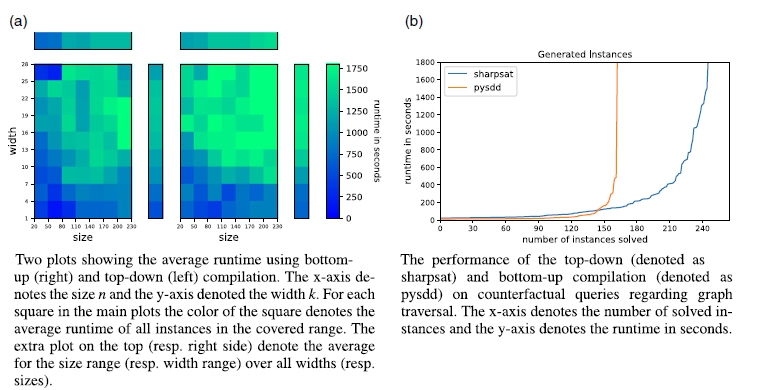
Fig. 1. Results for Q1.
In Figure 1a, we see that the average runtime depends on both the size and the width for either KC approach. This is especially visible in the subplots on top (resp. right) of the main plot containing the average runtime depending on the size (resp. width). While there is still a lot of variation in the main plots between patches of similar widths and sizes, the increase in the average runtime with respect to both width and size is rather smooth.
As expected, given the number of instances solved overall, top-down KC scales better to larger instances than bottom-up KC with respect to both size and structure. Interestingly however, for bottom-up KC the width seems to be of higher importance than for top-down KC. This can be observed especially in the average plots on top and to the right of the main plot again, where the change with respect to width is much more rapid for bottom-up KC than for top-down KC. For bottom-up KC, the average runtime goes from $\sim$
500 s to
$\sim$
500 s to $\sim$
1800 s within the range of widths between 1 and 16, whereas for top-down KC it stays below
$\sim$
1800 s within the range of widths between 1 and 16, whereas for top-down KC it stays below $\sim$
1500 s until width 28. For the change with respect to size on the other hand, both bottom-up and top-down KC change rather slowly, although the runtime for bottom-up KC is generally higher.
$\sim$
1500 s until width 28. For the change with respect to size on the other hand, both bottom-up and top-down KC change rather slowly, although the runtime for bottom-up KC is generally higher.
Q2. Number & Type of Evidence/Intervention The results for the effect of the number and types of evidence and intervention atoms are shown in Figure 2.
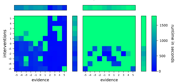
Fig. 2. Two plots showing the runtime using bottom-up (right) and top-down (left) compilation with varying evidence and intervention. The x-axis denotes the signed number of interventions, that is, $-n$
corresponds to n negative interventions and n corresponds to n positive interventions. The y-axis denotes the signed number of evidence atoms using analogous logic. For each square in the main plots, the color of the square denotes the runtime of the instance with those parameters. The extra plot on the top (resp. right side) denotes the average for the number and type of evidences (resp. interventions) over all interventions (resp. evidences).
$-n$
corresponds to n negative interventions and n corresponds to n positive interventions. The y-axis denotes the signed number of evidence atoms using analogous logic. For each square in the main plots, the color of the square denotes the runtime of the instance with those parameters. The extra plot on the top (resp. right side) denotes the average for the number and type of evidences (resp. interventions) over all interventions (resp. evidences).
Here, for both bottom-up and top-down KC, we see that most instances are either solvable rather easily (i.e. within 500 s) or not solvable within the time limit of 1800 s. Furthermore, in both cases negative interventions, that is, interventions that make an atom false, have a tendency to decrease the runtime, whereas positive interventions, that is, interventions that make an atom true, can even increase the runtime compared to a complete lack of interventions.
However, in contrast to the results for Q1, we observe significantly different behavior for bottom-up and top-down KC. While positive evidence can vastly decrease the runtime for top-down compilation such that queries can be evaluated within 200 s, even in the presence of positive interventions, there is no observable difference between negative and positive evidence for bottom-up KC. Additionally, top-down KC seems to have a much easier time exploiting evidence and interventions to decrease the runtime.
We suspect that the differences stem from the fact that top-down KC can make use of the restricted search space caused by evidence and negative interventions much better than bottom-up compilation. Especially for evidence, this makes sense: additional evidence atoms in bottom-up compilation lead to more SDDs that need to be compiled; however, they are only effectively used to restrict the search space when they are conjoined with the SDD for the query in the last step. On the other hand, top-down KC can simplify the given propositional theory before compilation, which can lead to a much smaller theory to start with and thus a much lower runtime.
The question why only negative interventions seem to lead to a decreased runtime for either strategy and why the effect of positive evidence is much stronger than that of negative evidence for top-down KC is harder to explain.
On the specific benchmark instances that we consider, negative interventions only remove rules, since all rule bodies mention r(x) positively. On the other hand, positive interventions only remove the rules that entail them, but make the rules that depend on them easier to apply.
As for the stronger effect of positive evidence, it may be that there are fewer situations in which we derive an atom than there are situations in which we do not derive it. This would in turn mean that the restriction that an atom was true is stronger and can lead to more simplification. This seems reasonable on our benchmark instances, since there are many more paths through the generated networks that avoid a given vertex, than there are paths that use it.
Overall, this suggests that evidence is beneficial for the performance of top-down KC. Presumably, the performance benefit is less tied to the number and type of evidence atoms itself and more tied to the strength of the restriction caused by the evidence. For bottom-up KC, evidence seems to have more of a negative effect, if any.
While in our investigation interventions caused a positive or negative effect depending on whether they were negative or positive respectively, it is likely that in general their effect depends less on whether they are positive or negative. Instead, we assume that interventions that decrease the number of rules that can be applied are beneficial for performance, whereas those that make additional rules applicable (by removing an atom from the body) can degrade the performance.
7 Conclusion
The main result in this contribution is the treatment of counterfactual queries for ProbLog programs with unique supported models given by Procedure 2 together with the proof of its correctness in Theorem 3. We also provide an implementation of Procedure 2 that allows us to investigate the scalability of counterfactual reasoning in Section 6. This investigation reveals that typical approaches for marginal inference can scale to programs of moderate sizes, especially if they are not too complicated structurally. Additionally, we see that evidence typically makes inference easier but only for top-down KC, whereas interventions can make inference easier for both approaches but interestingly also lead to harder problems. Finally, Theorems 4 and 5 show that our approach to counterfactual reasoning is consistent with CP-logic for LPAD-programs. Note that this consistency result is valid for arbitrary programs with stratified negation. However, there is no theory for counterfactual reasoning in these programs. In our opinion, interpreting the results of Procedure 2 for more general programs yields an interesting direction for future work.
Supplementary material
To view supplementary material for this article, please visit http://doi.org/10.1017/S1471068423000133.


 Open access