


INTRODUCTION
The postglacial vegetation history of the Northern Great Basin (NGB) has been strongly affected by the balance of moisture from the Pacific Ocean and continental dry and warm air masses moving north from the Central Great Basin (Wigand and Rhode, Reference Wigand, Rhode, Herschler, Madsen and Currey2002; Minckley et al., Reference Minckley, Whitlock and Bartlein2007). Although large lakes persisted in the basins of the NGB through the late Pleistocene, decreased effective moisture and increased evapotranspiration since 11,000 cal yr BP have resulted in the desiccation of these pluvial lakes and subsequent deflation of Pleistocene sediments, generally precluding the use of these larger basins as reliable archives of postglacial climate change (Allison, Reference Allison1982; Cohen et al., Reference Cohen, Palacios-Fest, Negrini, Wigand and Erbes2000). Understanding postglacial environments and reconstructing the heterogeneity of this landscape has implications for understanding the environments experienced by humans and other animals, which is especially important, as the NGB has evidence of some of the oldest human activity in North America (Gilbert et al., Reference Gilbert, Jenkins, Gotherstrom, Naveran, Sanchez, Hofreiter and Thomsen2008; Jenkins et al., Reference Jenkins, Davis, Stafford, Campos, Hockett, Jones and Cummings2012; McDonough, Reference McDonough2019), as well as extinct and extant megafauna remains (McDonough et al., Reference McDonough, Luthe, Swisher, Jenkins, O'Grady and White2012; Jenkins et al., Reference Jenkins, Davis, Stafford, Campos, Connolly, Cummings, Hofreiter, Graf, Ketron and Waters2013).
Many postglacial pollen records recovered from within the NGB have been studied at mid- to high-elevation sites, as low-elevation sites containing undisturbed sedimentary sequences that span the Holocene are uncommon (Cohen et al., Reference Cohen, Palacios-Fest, Negrini, Wigand and Erbes2000). The few low-elevation pollen records that do exist reveal the ubiquitous presence of xeric shrub–steppe vegetation since the last glacial maximum (Mehringer, Reference Mehringer1987; Wigand, Reference Wigand1987; Wigand and Rhode, Reference Wigand, Rhode, Herschler, Madsen and Currey2002; Mensing et al., Reference Mensing, Sharpe, Tunno, Sada, Thomas, Starratt and Smith2013; Beck et al., Reference Beck, Bryant and Jenkins2018; Kennedy, Reference Kennedy2018; McDonough et al., Reference McDonough, Kennedy, Rosencrance, Holcomb, Jenkins and Puseman2022). However, wetlands are embedded within this xeric landscape. In various places, drainages from mountains feed into seasonal or persistent wetlands, resulting in a sharp contrast between wet and xeric plant communities, as hydrophytic plants respond rapidly to changes in water availability (Kovalchik and Chitwood, Reference Kovalchik and Chitwood1990; Nowak et al., Reference Nowak, Nowak, Tausch and Wigand1994).
Terrestrial caves often serve as natural subaerial sediment traps and can preserve organic materials for thousands of years (White, Reference White2007). Archaeological investigations of caves and rock shelters occasionally yield preserved mammalian coprolites, offering opportunities to gain information about the diet and health of animals and to make inferences about past climates and environments (Bryant, Reference Bryant1974; Hofreiter et al., Reference Hofreiter, Poinar, Spaulding, Bauer, Martin, Possnert and Pääbo2000; Carrión et al., Reference Carrión, Riquelme, Navarro and Munuera2001; Gilbert et al., Reference Gilbert, Jenkins, Gotherstrom, Naveran, Sanchez, Hofreiter and Thomsen2008; Riley, Reference Riley2008; Shillito et al., Reference Shillito, Bull, Matthews, Almond, Williams and Evershed2011; Wood and Wilmshurst, Reference Wood and Wilmshurst2012, Reference Wood and Wilmshurst2016; Beck et al., Reference Beck, Bryant and Jenkins2018, Reference Beck, Bryant and Jenkins2020; Blong et al., Reference Blong, Adams, Sanchez, Jenkins, Bull and Shillito2020). Coprolite studies have been an important component of Great Basin archaeological research since the early twentieth century (Loud and Harrington, Reference Loud and Harrington1929; Heizer, Reference Heizer1969; Heizer et al., Reference Heizer, Napton, Dunn, Follett, Morbeck, Radovsky and Watkins1970; Kelso, Reference Kelso1971; Thomas et al., Reference Thomas, Davis, Grayson, Melhorn, Thomas, Trexler and Adovasio1983) and have since greatly expanded our understanding of past human behaviors and health (Jenkins et al., Reference Jenkins, Davis, Stafford, Campos, Hockett, Jones and Cummings2012, Reference Jenkins, Davis, Stafford, Campos, Connolly, Cummings, Hofreiter, Graf, Ketron and Waters2013; Dexter and Saban, Reference Dexter and Saban2014; Beck et al., Reference Beck, Bryant and Jenkins2018; Kennedy, Reference Kennedy2018; McDonough, Reference McDonough2019; Blong et al., Reference Blong, Adams, Sanchez, Jenkins, Bull and Shillito2020; McDonough et al., Reference McDonough, Kennedy, Rosencrance, Holcomb, Jenkins and Puseman2022).
Located in south-central Oregon within the NGB, the Paisley 5-Mile Point archaeological site (Paisley Caves) produced a material assemblage that includes abundant coprolites, providing opportunities for expanding the interpretation of pollen records from cave sediments. More than 2800 mammalian coprolites were excavated from Paisley Caves between 2002 and 2011 (Jenkins et al., 2012, 2013), and each represents a point in time during the last 14,300 yr. In this study, we assess the environmental conditions present during periods of wetland expansion and subsequent lake retreat in the Summer Lake basin between 14,000 and 6000 cal yr BP by comparing pollen assemblages of coprolites and their associated sediments. With this approach, pollen recovered from sediments represents multidecadal periods of sedimentation, while coprolite pollen offers a different view of environmental conditions due to a short (several-day) “sampling” period. The Paisley Caves are situated in close proximity to three ecotones: lacustrine–wetland, sagebrush steppe, and conifer forest (Cronquist et al., Reference Cronquist, Holmgren, Holmgren and Reveal1972; Franklin and Dyrness, Reference Franklin and Dyrness1988; Anderson et al., Reference Anderson, Borman and Krueger1998). Contrasting pollen assemblages of sediments and coprolites may help clarify the paleovegetation history, which is still not well understood at low-elevation NGB sites.
Five previous studies of pollen and macrobotanical assemblages were conducted at Paisley Caves. First, Saban (Reference Saban2015) produced a pollen record from the same sampling unit (Cave 2, Unit 6B) as this study and is succeeded by the present study. Second, Beck et al. (Reference Beck, Bryant and Jenkins2018) produced a pollen record from the same cave as this study (Cave 2), but located 1 m north of our sampled profile at a site with a different chronology and potentially different taphonomic processes (e.g., exposure to wind). Third, Kennedy (Reference Kennedy2018) identified macrobotanical remains from Cave 2 and developed a detailed description of local vegetation and cultural foods and plant resources. Fourth, Beck et al. (Reference Beck, Bryant and Jenkins2020), at the same profile as Beck et al. (Reference Beck, Bryant and Jenkins2018), compared Neotoma spp. (packrat) coprolite pollen assemblages with sediment pollen assemblages. Due to the small mass of Neotoma coprolites, Beck et al. (Reference Beck, Bryant and Jenkins2020) merged 57 coprolites into single samples resulting in a total of fifteen 0.25 g samples of packrat coprolites. Pollen assemblages of Neotoma coprolites were statistically very similar to those in associated sediments, but coprolite pollen assemblages were more variable than those from sediments, possibly due to meal choice (Beck et al., Reference Beck, Bryant and Jenkins2020). Finally, Blong et al. (Reference Blong, Adams, Sanchez, Jenkins, Bull and Shillito2020) examined contents of nine coprolites identified as originating from humans from the Younger Dryas (YD) through the Early Holocene for the purpose of reconstructing prehistoric human diets. That study found seeds, bones of small mammal and fish, and beetle remains in the coprolites, supporting foraging in marshes. Blong et al. (Reference Blong, Adams, Sanchez, Jenkins, Bull and Shillito2020) also conducted limited pollen analyses, which found elevated percentages of insect-pollenated taxa and pollen aggregates, suggesting direct consumption of pollen.
DNA analysis of other coprolites from Paisley Caves have revealed coprolites associated with Homo sapiens, Camelidae, Lynx, Ovis, and Panthera (Jenkins et al., Reference Jenkins, Davis, Stafford, Campos, Hockett, Jones and Cummings2012). In addition to preserving the oldest human coprolites in North America, the Paisley Caves boast an extensive assortment of organic artifacts and materials that offer invaluable insights into the activities of humans and fauna from more than 14,000 yr ago. However, our comprehension of how humans and large mammals traversed the ancient landscapes of the NGB remains limited. Given the limited past analyses of mammalian coprolite pollen at Paisley Caves (Blong et al., Reference Blong, Adams, Sanchez, Jenkins, Bull and Shillito2020), there remains a potential for this approach to provide us with a better understanding of how large mammals roamed the local environment and left behind evidence of their movements at the caves.
Traditionally, mammalian coprolite analysis from archaeological sites in North America has been used to reconstruct diet, health (Bryant and Holloway, Reference Bryant and Holloway1983; Bryant and Reinhard, Reference Bryant, Reinhard, Hunt, Milan, Lucas and Spielmann2012; Blong et al., Reference Blong, Adams, Sanchez, Jenkins, Bull and Shillito2020), and human activities at a site (Gilbert et al., Reference Gilbert, Jenkins, Gotherstrom, Naveran, Sanchez, Hofreiter and Thomsen2008; Jenkins et al., Reference Jenkins, Davis, Stafford, Campos, Hockett, Jones and Cummings2012; McDonough, Reference McDonough2019; Shillito et al., Reference Shillito, Blong, Green and van Asperen2020). This study uses coprolite pollen solely as an environmental proxy to reconstruct conditions at and beyond the caves. Pollen found in coprolites represents short periods of time, approximately 19–37 hours (Kelso and Solomon, Reference Kelso and Solomon2006), and is derived from various sources: pollen in drinking water, airborne pollen that entered nasal and esophageal mucus, pollen adhered to any food item, pollen in ingested flowers or pollen cones, or pollen in the stomach content of prey (Carrión et al., Reference Carrión, Riquelme, Navarro and Munuera2001; Chame, Reference Chame2003). Thus, coprolite pollen represents a brief period that can potentially reveal different information than sediment pollen. This study is unique in using coprolites as distinct pollen samples for direct statistical comparison to contemporaneous sediments and considering all taphonomic pathways (not only diet) behind the formation of the coprolite pollen assemblage (Shillito et al., Reference Shillito, Blong, Green and van Asperen2020).
Interpretation of pollen assemblages from cave sediments can be limited for several reasons. Caves often contain both eolian and slopewash sediment, filtered from the environment via the single depositional entry of the cave opening. Also, within the NGB, redeposition of sediments blown off dry lakebeds may contribute pollen from prior climatic periods (Anderson, Reference Anderson1955). The location of the sediment samples relative to the layout of the cave may affect pollen assemblages due to, for example, pollen degradation caused by temperature exposure or physical degradation within a drip zone. Finally, bioturbation of sediments by faunal or human activities can disturb or erase the chronological integrity of sedimentary sequences, resulting in time-averaged pollen assemblages.
We hypothesize that differences in the pollen assemblages between cave sediment and coprolites emerge primarily due to the unique sampling of the environment by a mammal. We therefore predict that (1) pollen assemblages will differ more between coprolites and associated sediments than between samples within either group; (2) pollen assemblage turnover (i.e., rate of change) will be greater for coprolites than in sediments due to the potentially stochastic processes that determine the coprolite pollen assemblage; and (3) pollen taxonomic diversity will be greater in sediments than in coprolites, as sediments sample a larger spatial and temporal window of pollen deposition than do coprolites.
STUDY AREA
Geologic setting
Summer Lake basin is located within the larger Chewaucan Basin, a V-shaped graben delineated by steep fault scarps and subdivided into three subbasins: Summer Lake lies in the northwest portion of the V, with the basin that holds Upper and Lower Chewaucan Marshes in the south, and Lake Abert in the northeast (Fig. 1). The Chewaucan Basin graben dips northwest, with the Summer Lake basin floor averaging 1275 m above sea level (m asl), Upper and Lower Chewaucan Marshes averaging 1314 m, and the Lake Abert basin averaging 1299 m asl.

Figure 1. (A) Location of 5-Mile Point Butte and Paisley Caves in the Chewaucan Basin of south-central Oregon. Black line shows the maximum high-water extent of pluvial lakes during the late Pleistocene. (B) View of 5-Mile Point Butte, facing east. (C) View of Winter Rim from Cave 5, Paisley Caves, facing west.
The Paisley Caves are located on 5-Mile Point Butte, a scoriaceous basalt fault block butte located in the southeastern part of Summer Lake basin in south-central Oregon. This site is approximately 18 km east of the current Summer Lake shoreline and 8 km north of the Chewaucan River (Fig. 1). The caves are all on a southwest aspect, and their entrances are located midway up the butte at an average elevation of 1366 m asl (Fig. 1B). A series of eight wave-cut caves and rock shelters formed as a result of energetic wave action by Lake Chewaucan during periods of stable high lake stands (Allison, Reference Allison1982; Friedel, Reference Friedel1993; Jenkins et al., Reference Jenkins, Davis, Stafford, Campos, Connolly, Cummings, Hofreiter, Graf, Ketron and Waters2013). Subsequent rockfalls at cave entrances have since resulted in some of the deeper caves developing into shallow rock shelters.
The current dry lakebed near 5-Mile Point Butte dips west at a 3.3° slope until the lakebed abruptly ends at the base of Winter Rim. The topography of the area north of 5-Mile Point Butte is characterized by dry lake flats, deflated playas, lunettes, and dune systems, with some small basalt fault block outcrops. East of 5-Mile Point Butte the topography rises in elevation above the lakebed floor and is less steep than the west side of Summer Lake basin. This east side is composed of fault block features that increase in elevation for 13 km up to approximately 1590 m, after which the topography then slopes down 13 km east to Lake Abert. The Summer Lake lakebed slopes little south of 5-Mile Point Butte, where the topography is interrupted by the incised course of a stream that resulted from the overflow of ZX Lake into Summer Lake during the YD (Allison, Reference Allison1982; Friedel, Reference Friedel1993; Licciardi, Reference Licciardi2001; Hudson et al., Reference Hudson, Emery-Wetherell, Lubinski, Butler, Grimstead and Jenkins2021).
Pluvial Lake Chewaucan covered an area of 1243 km2 at its maximum extent, with a surface elevation of 1381 m asl and a maximum depth of ca. 118 m (Allison, Reference Allison1982; Cohen et al., Reference Cohen, Palacios-Fest, Negrini, Wigand and Erbes2000). The primary stream feeding Lake Chewaucan was the Chewaucan River, draining north through a steep river valley into the Chewaucan Basin. During the late Pleistocene Bølling-Allerød (BA) period, 14,700 to 12,900 cal yr BP (Sowers and Bender, Reference Sowers and Bender1995), water levels in Lake Chewaucan reached their last high stand by ca.14,500 cal yr BP, after which levels declined and Chewaucan River sediments formed the Paisley Fan (1323 m asl) at the south end of Summer Lake, resulting in Summer Lake hydrologically separating from the rest of the Chewaucan basin (Allison, Reference Allison1982; Licciardi, Reference Licciardi2001). Basal sediments in this current study were dated to ca. 14,000 cal yr BP, the time of the Chewaucan high stand.
The YD cold period (12,800–11,600 cal yr BP) is characterized by a return to cooler temperatures in the Northern Hemisphere (Mayewski et al., Reference Mayewski, Meeker, Whitlow, Twickler, Morrison, Alley, Bloomfield and Taylor1993; Rasmussen et al., Reference Rasmussen, Bigler, Blockley, Blunier, Buchardt, Clausen and Cvijanovic2014). At this time, Summer Lake began receding due to lower precipitation and increasing summer insolation (Hudson et al., Reference Hudson, Hatchett, Quade, Boyle, Bassett, Ali and De los Santos2019, Reference Hudson, Emery-Wetherell, Lubinski, Butler, Grimstead and Jenkins2021). The climate began to warm after the YD, eventually resulting in climatic conditions being warmer during the earliest portions of the Holocene (11,000–9000 cal yr BP), with evidence of a brief period of increased precipitation that resulted in a transgression of Summer Lake to moderately high levels, although not as high as during the BA (Hudson et al., Reference Hudson, Emery-Wetherell, Lubinski, Butler, Grimstead and Jenkins2021). Conditions reached thermal and aridity maxima after 9000 cal yr BP, after which climatic conditions began to cool but remained arid (Friedel, Reference Friedel1993; Bartlein et al., Reference Bartlein, Anderson, Anderson, Edwards, Mock, Thompson, Webb and Whitlock1998, Reference Bartlein, Harrison, Brewer, Connor, Davis, Gajewski and Guiot2011; Cohen et al., Reference Cohen, Palacios-Fest, Negrini, Wigand and Erbes2000; Benson et al., Reference Benson, Kashgarian, Rye, Lund, Paillet, Smoot, Kester, Mensing, Meko and Lindström2002; Mensing et al., Reference Mensing, Benson, Kashgarian and Lund2004; Minckley et al., Reference Minckley, Whitlock and Bartlein2007; Long et al., Reference Long, Shinker, Minckley, Power and Bartlein2019; Hudson et al., Reference Hudson, Emery-Wetherell, Lubinski, Butler, Grimstead and Jenkins2021).
Climate and vegetation
The Summer Lake basin is presently located at a convergence zone of moist Pacific air parcels moving inland from the southwest and continental climate characterized by a high-pressure system centered above the Central Great Basin in Nevada to the southeast of the Chewaucan Basin, which have varied over the Holocene (Reinemann et al., Reference Reinemann, Porinchu, Bloom, Mark and Box2009; Carter et al., Reference Carter, Brunelle, Minckley, Shaw, DeRose and Brewer2017; Long et al., Reference Long, Shinker, Minckley, Power and Bartlein2019). Geographically located in the rain shadow of the Cascade Range, the NGB region currently has warm summers and cold winters (mean July and January temperatures 17.7°C and 2.2°C, respectively). Average annual precipitation is 33.9 cm; most precipitation occurs from November through January, with afternoon thunderstorms during summer seasons.
Vegetation gradients in the region are primarily determined by elevation and its effects on orographic precipitation (Franklin and Dyrness, Reference Franklin and Dyrness1988; Kovalchik and Chitwood, Reference Kovalchik and Chitwood1990; Osmond et al., Reference Osmond, Hidy and Pitelka1990). Current Summer Lake basin vegetation is high desert shrub–steppe dominated by Artemisia tridentata and salt-tolerant Amaranthaceae (Chenopodium and Atriplex; Franklin and Dyrness, Reference Franklin and Dyrness1988; St. Louis, Reference St. Louis2021). The A. tridentata community includes an understory of the invasive Bromus tectorum, as well as Elymus sp., Ericameria teretifolia, Sarcobatus vermiculatus, and various other shrubs, forbs, and grasses adapted to sandy eolian sediments and highly alkaline aridisols. At the base of 5-Mile Point Butte, the lakebed sharply transitions into a steep, rocky talus of basalt boulders with pockets of playa loess accumulating between the boulder gaps. Vegetation on the talus slope is primarily Artemisia and Chrysothamnus sp. with intermittent cespitose Eriogonum sp. and hemiparasitic Castilleja angustifolia.
The trees currently nearest to the caves are 8 km to the south at the town of Paisley, where riparian vegetation extends along the Chewaucan River into Upper Chewaucan Marsh. Modern-day trees and shrubs include Pinus ponderosa, Alnus incana, Betula occidentalis, Juniperus occidentalis, Prunus virginiana, Salix sp., Populus tremuloides, Populus trichocarpa, and non-native Populus alba. A very small population of Quercus garryana var. semota was reported on Gearhart Mountain at 1650 m asl (https://oregonflora.org/taxa/index.php?taxon=14318). Nonnative Medicago sativa is grown in center-pivot irrigation fields within a few kilometers of the caves. Marsh plants are present in both the Upper and Lower Chewaucan Marshes, near the Summer Lake Hot Springs ca. 8 km west of 5-Mile Point Butte, along most of the 40 km base of Winter Rim, and at the north end of the Summer Lake basin at the Summer Lake Wildlife Area 24 km north of 5-Mile Point Butte. The marsh communities include a range of Poaceae, Juncaceae, Cyperaceae, Ribes sp., Typhaceae, and Asteraceae. Trees present 20 km west of 5-Mile Point Butte on the steep scarp of Winter Rim (2200 m elevation) include P. trichocarpa and P. alba, P. virginiana at the base; P. ponderosa, Salix sp., J. occidentalis, P. tremuloides at mid-elevation; and Pinus contorta and Abies concolor at the Winter Rim summit.
Archaeological excavations at Paisley Caves
Sediments and coprolites used in this study were all collected during archaeological research at Paisley Caves between 2009 and 2011. Archaeological research began in 1938 under University of Oregon archaeologist Luther S. Cressman (Cressman, Reference Cressman1940; Jenkins et al., Reference Jenkins, Connolly, Aikens, Jenkins, Connolly and Aikens2004), who numbered the caves sequentially from south to north. From 2002 to 2011, DLJ directed further excavations at the site for the University of Oregon. Materials recovered ranged from artifacts such as lithic tools and debitage, bone, antler, and wood tools, cordage, and grinding stones (manos and metates), as well as a rich array of organic materials that included plant macrofossils; insects; the bones of fish, waterfowl, small mammals, extant and extinct megafauna, and reptiles; and 2533 coprolites of human and other mammalian origins. Gilbert et al. (Reference Gilbert, Jenkins, Gotherstrom, Naveran, Sanchez, Hofreiter and Thomsen2008) reported on the DNA sequencing of three ca. 14,000-yr-old human coprolites, which at the time of publication were the oldest confirmed human remains in the Western Hemisphere.
Materials dated to the YD period showed human activity was very high in Paisley Cave 2, with cultural material deposits becoming dense enough to create a culturally formed stratigraphic level referred to as the Botanical Lens (BL). BL deposits are composed primarily of a 5- to 8-cm-thick mat of Artemisia twigs and shredded bark and contained a hearth dated to the YD (Jenkins et al., Reference Jenkins, Davis, Stafford, Campos, Connolly, Cummings, Hofreiter, Graf, Ketron and Waters2013). The BL is underlain by a 1–3 cm alluvial mud lens dated to ca. 12,930 cal yr BP and capped by a second 1–2 cm mud lens dated to ca. 11,500 cal yr BP.
The coprolites and sediments used in this study were excavated from Cave 2, Unit 2/6 (Fig. 2). Materials from this unit were selected for this project due to the high number of well-mapped, stratigraphically sequential, and large mammalian coprolites with associated sediments, as well as for the minimal westward slope of the cave floor (Fig. 3). Cave 2 is approximately 7 m long, 6 m wide, and 3 m deep; 30.3 m3 of sediment over 22 m2 has been excavated from this cave (Jenkins et al., Reference Jenkins, Davis, Stafford, Campos, Connolly, Cummings, Hofreiter, Graf, Ketron and Waters2013). The cave walls are composed of fine-grained basalts mixed with soft volcanic tuffs and breccias. Summer Lake basin is a seismically active area (Licciardi, Reference Licciardi2001; Badger and Watters, Reference Badger and Watters2004; Orr and Orr, Reference Orr and Orr2012) resulting in roof falls being common in the caves. Roof fall materials range from small pebbles to multi-ton boulders, the most notable of which was once the outer ceiling of Cave 2, which now blocks most of the entrance to the cave. The age of the roof fall is ca. 2,300 cal yr BP based on a radiocarbon date obtained from a human coprolite recovered from beneath a smaller boulder from the same event (Jenkins et al., Reference Jenkins, Davis, Stafford, Campos, Connolly, Cummings, Hofreiter, Graf, Ketron and Waters2013). In 1939, Luther Cressman excavated a trench in Cave 2 but missed unit 2/6 due to the presence of the roof-fall boulders. Looters who later dug up the Cressman trench also missed the 2/6 sediments for the same reason. The larger boulder remains in place, but the smaller one was removed in 2009. Cave 2 was divided into seven 2 m × 2 m plots that were further subdivided into 1 m × 1 m units (Fig. 2). By the end of Cave 2 excavations in 2011, the cave had been excavated in primarily 5 cm increments down to bedrock at a depth of ca. 308 cm.

Figure 2. Cave 2 showing location of Unit 6 relative to datum and roof-fall boulder at west end of entrance. Previous sediment sampling by Saban (Reference Saban2015) shown as small teal box and Beck et al. (Reference Beck, Bryant and Jenkins2018) sampling shown as small green triangle. Map image redrawn from Jenkins et al. (Reference Jenkins, Davis, Stafford, Campos, Hockett, Jones and Cummings2012).

Figure 3. Remaining west wall of unit 2/6. This sediment wall is overlain by the roof collapse that occurred ~2000 cal yr BP. Visible in the photo are the tephra layer; indurated laminations; the remains of a small hearth, which is part of the BL; and rodent holes (krotovina). Bottom image and description were redrawn from Jenkins et al. (Reference Jenkins, Davis, Stafford, Campos, Hockett, Jones and Cummings2012).
Sediment description
Cave 2 sediments are composed of both biological and exogenetic materials (Jenkins et al., Reference Jenkins, Davis, Stafford, Campos, Hockett, Jones and Cummings2012) and include varying amounts of eolian deposits, rockfall, bat guano, rodent feces, deposited cultural materials, and vegetation blown in or brought into the rock shelter by Neotoma sp. Areas under smaller rockfall boulders not excavated by Cressman in 1938 were bioturbated by rodents or badgers or destroyed by looters in places, but overall the sediment matrices were well preserved and in excellent sequential order (Jenkins et al., Reference Jenkins, Davis, Stafford, Campos, Hockett, Jones and Cummings2012). This was largely due to millennia of urine accumulation forming hydrophobic and waterproof indurated sediments (Jenkins et al., Reference Jenkins, Davis, Stafford, Campos, Hockett, Jones and Cummings2012). A cross-section of the remaining 2/6 west sediment wall (Fig. 3) shows the stratigraphy before excavations. Cave 2 has an average sedimentation rate of approximately 50 yr/cm, with the exception of the BL, which is primarily of anthropogenic origin, and the 30 cm of Mazama tephra representing a single event (Jenkins et al., Reference Jenkins, Davis, Stafford, Connolly, Jones, Rondeau, Cummings, Kornfeld and Huckell2016).
Lithostratigraphic units (LUs) are distinct sediment types that make up the matrices of sedimentary units and are defined by their sediment characteristics (Gasche and Tunca, Reference Gasche and Tunca1983; Stein, Reference Stein1987). Seven LUs were identified in Cave 2 (Fig. 3), although only three are relevant here. LU1 overlays basement rock in a portion of 2/6B that was not sampled for this project. LU2 is a dark-brown, poorly sorted gravelly sand approximately 30 cm thick overlying basement rock or LU1. A distinct transition from LU2 to LU3 occurs at ca. 260 cm and has been dated to 12,500 cal yr BP. The transition is marked by a patchy occurrence of the BL (described earlier) and includes a small hearth of charred organic material overlain by ashy/organic sediment. LU3 extends up to the cataclysmic eruption of Mount Mazama 7633 cal yr BP (Egan 2015). LU3 is a mix of fine eolian-deposited sediments, some smaller poorly sorted gravels mixed with angular roof fall, and heavy organic components of plant materials and bat guano (Jenkins et al., Reference Jenkins, Davis, Stafford, Campos, Hockett, Jones and Cummings2012). LU3 sediments are firm to hard, of polygenetic origins with abundant macrobotanical content, amorphous organic matter, and high amounts of Neotoma and Chiroptera feces (Jenkins et al., Reference Jenkins, Davis, Stafford, Campos, Hockett, Jones and Cummings2012). Weakly consolidated Mazama tephra (152–180 cm) was assigned as LU4. Guano pellets from the base of the Mazama tephra were dated to 7633 cal yr BP (Jenkins et al., Reference Jenkins, Davis, Stafford, Campos, Connolly, Cummings, Hofreiter, Graf, Ketron and Waters2013). Laminations and fine ash capping and underlying the tephra suggests primary tephra deposition at the west end of Unit 2/6 (Fig. 3). The tephra in the 2/6 west wall ranges from fine ash to pale yellow rhyolitic lapilli from 1 to 1.5 mm in size. The topmost sediments for this unit are referred to as LU5 and contained little to no Mazama tephra (Jenkins et al., Reference Jenkins, Davis, Stafford, Campos, Hockett, Jones and Cummings2012).
MATERIAL AND METHODS
Material collection during excavations
All coprolites found in situ during excavations in Cave 2 from 2009 to 2011 were collected following strict protocols to limit their exposure to modern-day DNA contamination. These collection protocols included Tyvek hazmat suits, sterile gloves, forceps, and specimen cups. For most of the sampled coprolites, a sediment sample was also taken directly below the coprolite. Both samples were then sealed into sterile specimen cups and labeled. All coprolites selected for the study had an associated sample of sedimentary materials collected at the same time. No effort was made to distinguish human coprolites from those of other large carnivorous or omnivorous mammals. The coprolites were desiccated and ranged from very light tan to medium brown (Fig. 4). Faunal fragment analysis resulted in 6 to 20 bone fragments per coprolite sample, ranging from 3 to 8 mm in size, and included mammalian and avian bone fragments (Cromwell, R.P., personal communication, 2016). All the bones were fragmented except for one rodent left tarsal, several rodent molars, the dentin sheath of a rodent incisor, and two rodent claws. Positions of artifacts and radiocarbon dates were changed from elevation (m) to centimeters below the modern cave floor (1368.3 m) for subsequent analyses. All samples in this study are from unit 6B (Fig. 2). In this portion of the cave, undisturbed sediments were excavated at depths of 120 to 320 cm below the 1368.3 m asl elevation.

Figure 4. Examples of coprolite specimens used in this study. Colors range from light tan to dark brown. Photographs were taken in 2016.
Lab processing
Coprolites
Sampling and chemical processing of both coprolites and sediments was conducted at the University of Oregon, where strict sampling procedures were followed to protect the remaining materials from modern DNA contamination. Coprolites were subsampled for pollen following methods outlined by Wood and Wilmshurst (Reference Wood and Wilmshurst2012, Reference Wood and Wilmshurst2016), except for sectioning the coprolites along a longitudinal axis rather than the center. An average dry weight of 1.6 g (ranging from 0.668 to 3.638 g) was sampled from the center of each coprolite (Fig. 4). Coprolites lighter than 0.50 g were not processed.
The chemical process for pollen recovery from coprolites followed Pearsall (Reference Pearsall2016) and Smith (Reference Smith, Wrenn and Bryant1998) but was modified to protect materials, including bone and plant fibers, for possible future radiocarbon dating. Chemical pollen extraction was performed inside a fume hood. Each coprolite subsample was placed in a 50 mL tube and spiked with one Lycopodium tablet to determine pollen concentration. Samples were rehydrated with 50 mL warm 10% sodium hexametaphosphate (Na6[(PO3)6]) for 48–72 hours. Samples were sieved at 180 μm, and macrofossils were collected. Samples were treated with a 10% potassium hydroxide (KOH) at 80°C for 10 minutes, acetolysis (9:1 acetic anhydride:sulfuric acid, heated for 3 minutes). Samples were stained with Safranin and desiccated using ethyl alcohol and tert-butyl alcohol. Pollen was transferred into 2-dram glass vials with silicone oil used for suspension and preservation of pollen (Faegri et al., Reference Faegri, Kaland and Krzywinski1989).
Cave sediment
Pollen recovery from the Paisley sediments required some minor adjustments to the chemical extraction process from Smith (Reference Smith, Wrenn and Bryant1998) and Pearsall (Reference Pearsall2016). Sediments were wet sieved using a 125 μm mesh until 20 cm3 of the fine fraction was obtained. Each sample was added to a 1000 mL Nalgene beaker (12 samples per lab session) and spiked with one Lycopodium tablet to measure pollen concentrations. Samples were soaked in warm 10% Na6[(PO3)6]. Sediments were agitated and allowed to settle for 8 hours, after which the water was partially decanted and replaced with distilled water (no additional Na6[(PO3)6] added), agitated, and allowed to settle for another 8 hours. This process was repeated for approximately 10–12 days until the water was clear. Then, 10% KOH (80°C, 10 minutes) was used to remove remaining soluble organics followed by a 10% hydrochloric acid (HCl) treatment to remove carbonate minerals. A cold hydrofluoric acid (HF) treatment for 24 hours reduced silicate content. Prior work on Cave 2 sediments showed that a cold HF treatment was more effective at removing silicates than a 45 minute hot HF treatment (Saban, Reference Saban2015). Following a second 10% HCl treatment, the samples were rinsed with ultrapure water.
Following the Smith (Reference Smith, Wrenn and Bryant1998) protocols for processing dry sediments, a heavy liquid solution (1.9–2.0 specific gravity) of zinc bromide (ZnBr2) was used to separate pollen from heavier materials. Following centrifuging, pollen suspended on the heavy liquid was decanted into 50 mL centrifuge tubes. ZnBr2 heavy liquid suspension was repeated twice per sample. The remaining sediments in their original centrifuge tubes were filled with ultrapure water, capped, and placed into storage boxes for possible future pollen recovery. The pollen fractions were diluted with water and centrifuged to remove the remaining ZnBr2. Pollen was then transferred into 15 mL centrifuge tubes. Glacial acetic acid was used to remove water, followed by acetolysis (as for the coprolite samples) to remove the remaining cellulose. Samples were stained, desiccated, and suspended in silicone oil as described for the coprolite pollen.
Identifications
Pollen from both coprolites and sediments were examined at 400× magnification. Pollen was identified to the highest taxonomic resolution possible using published keys (Faegri et al., Reference Faegri, Kaland and Krzywinski1989) and the modern pollen reference collection at the University of Oregon. Both coprolite and sediment slides were counted to a minimum of 350 grains per sample, except for one coprolite with low pollen abundance, where only 175 pollen grains could be identified.
Chronology
An age–depth model was constructed using the INTCAL20 calibration curve and the Bacon R package (Blaauw and Christen, Reference Blaauw and Christen2011; Reimer et al., Reference Reimer, Austin, Bard, Bayliss, Blackwell, Ramsey and Butzin2020). The model is based on 16 radiocarbon dates available from unit 2/6 (Saban, Reference Saban2015; Jenkins et al., Reference Jenkins, Davis, Stafford, Connolly, Jones, Rondeau, Cummings, Kornfeld and Huckell2016). We also obtained a new date on an unidentified plant macrofossil from a coprolite occurring above the Mazama tephra. A date of 7633 cal yr BP for the Mount Mazama eruption (Egan et al., Reference Egan, Staff and Blackford2015) was included in the age–depth model. In the Bacon model, we specified the Mazama tephra unit as an instantaneous event and placed a hiatus at 296.5 cm, where an abrupt change in ages corresponds roughly to the depth of the BL.
Statistical analyses
Raw pollen counts were transformed into percentages and diagramed using Tilia 3.0.1. Pollen assemblage zones of the sediment pollen record were determined using stratigraphically constrained cluster analysis. We used the rioja package in R statistical software to identify zones based upon the chord distance, calculated as the Euclidean distance of square-root-transformed pollen proportions. The number of significant pollen zones was determined using the broken stick method (Bennett, Reference Bennett1996).
Nonmetric multidimensional scaling (NMDS) gradient analysis was used to compare sediment and coprolite assemblage relationships. NMDS is an indirect gradient ordination analysis using a dissimilarity matrix that describes a pairwise difference between taxa assemblages. Pollen assemblage dissimilarity was measured with the chord distance using the vegdist and metaMDS functions in the vegan package in R (Oksanen et al., Reference Oksanen, Blanchet, Kindt, McGlinn, Minchin, O'Hara, Simpson, Solymos, Stevens, Szoecs and Wagner2020). Both coprolites and sediments were included in the ordination, using the 29 taxa found in three or more samples.
Chord-distance dissimilarity was summarized between coprolites and adjacent sediment and between adjacent sediment and coprolite samples as a measure of stratigraphic turnover. Pollen taxa richness of coprolite and sediment samples was estimated with rarefaction for a sample of 175 pollen grains, using the rarefy function in vegan. The difference of rarefied pollen richness between coprolites and corresponding sediment samples was tested using a paired t-test.
RESULTS
Sediment age–depth model and pollen assemblage zones
Thirteen of the 17 radiocarbon ages occur in the lower 40 cm, surrounding the BL, and several were out of stratigraphic order. The Bacon age–depth model provides a best estimate of ages through periods of overlapping radiocarbon dates at the base of the section and also interpolates between ages at the top of the section (Fig. 5, Table 1). The basal age at 308 cm was modeled to 13,900 cal yr BP. Very slow accumulation occurred from 300 to 296 cm (encompassing 700 yr). Furthermore, a hiatus was required to fit the age model to a step change in the radiocarbon dates at 296.5 cm (12,700 to 12,200 cal yr BP), which corresponds to the BL between units LU2 and LU3. This hiatus does not appear to be present in other portions of Paisley Cave 2 (Beck et al. Reference Beck, Bryant and Jenkins2018). Instead of containing sediments, the BL is composed of organic materials, including artifacts, macrobotanicals, and coprolites. There were coprolites available from the BL, but as there were no corresponding sediments, they were not used in this study. Above this hiatus, fewer ages constrain the age model, but they show a generally fast sedimentation rate (20 yr/cm) that declined upward to the Mazama tephra (70 yr/cm).

Figure 5. Bacon age–depth model for Paisley Cave 2, Unit 6 (Blaauw and Christen, Reference Blaauw and Christen2011). The gray area on the graph represents sediments enriched with Mazama tephra. The top row of figures shows the evolution of the fit of the model, the prior and posterior distributions of the sedimentation accumulation rate, the temporal memory of the accumulation rate, and the duration of the hiatus (vertical dashed line).
Table 1. Radiocarbon dates from Paisley Cave 2, unit 6.

a Depths are with respect to a datum at 1367.70 m elevation.
Overall, pollen preservation was very good, with only <2% being indeterminable. The coprolites did not contain pollen aggregates, which have been interpreted as pollen being consumed directly (e.g., Blong et al., Reference Blong, Adams, Sanchez, Jenkins, Bull and Shillito2020). The stratigraphically constrained cluster analysis identified three zones in the sediment record, with breaks at 252 cm (11,100 cal yr BP) and 172 cm (within the Mazama-enriched sediment). The break at 252 cm corresponds roughly with the LU2/LU3 boundary. Pollen concentrations were sufficient for pollen analysis in the Mazama-enriched zone (LU4, 180–152 cm).
Sediment pollen record
P1: Late Pleistocene BA to Early Holocene
Period P1 covers a 2700-yr time span from 13,900 cal yr BP during the BA warm period, and following a sediment hiatus, to the Early Holocene (11,100 cal yr BP). A total of 20 taxa were identified (Fig. 6A). Common pollen types during P1 included Pinus subg. Pinus (increasing from 25% to 45%, then returning to 30%), Pinus subg. Strobus (1–2%), Abies (3–6%), Pseudotsuga (1–2%), Acer (1–2%), Betulaceae (1%), Salix (4–10%), Grossulariaceae (1%), Rhamnaceae (1%), Artemisia (15–28%), Ambrosia-type (11%, decreasing to 1%), Asteroideae-type (1%), Amaranthaceae (5%, increasing to 30%), Fabaceae (3–5%), Polygonaceae (3%), Onagraceae (1%), Typhaceae (3–4%), Alismastaceae (1%), and Poaceae (4%). Pollen concentrations declined from 120,000 grains/cm3 in the sample before the hiatus to 50,000 grains/cm3 after the hiatus, then increased to 80,000 grains/cm3.

Figure 6. (A) Pollen diagram from cave sediments from Paisley Cave 2 Unit 6. The diagram includes a surface sample taken at 10 cm below the modern surface immediately in front of Cave 2. The depth of the modeled hiatus (296.5 cm) is shown. (B) Pollen diagram for pollen in coprolites located adjacent to sediment samples. Pollen concentrations are grains per gram of dry mass.
P2a: Early Holocene to the Mazama tephra
P2a ranges from the Early Holocene at 11,100 cal yr BP to the Mazama tephra at 7633 cal yr BP. Thirty taxa were identified. Abies increased sharply from 7% to 21% at the start of P2a and remained at approximately 20% until the Mazama tephra. During this time, Artemisia declined from 24% to 10%. Pinus subg. Pinus pollen remained consistently between 28 and 35%, and Pinus subg. Strobus declined to below 1%. Conifers also included Picea (0–4%) and Pseudotsuga (1%). Other taxa included Taxaceae (1–2%), Cupressaceae (1–2%), Betulaceae (1–5%), Alnus undiff. (1–2%), Salix (1–5%), Populus undiff. (1–3%), Aceraceae (3%), Celestraceae (1%), Artemisia (9–20%), Asteroideae-type (1–5%), Ambrosia-type (1–4%), Amaranthaceae (8–23%), Brassicaceae (1–7%), Fabaceae (2–5%), Onagraceae (1–2%), Solanaceae (1%), Typhaceae (1–4%), Cyperaceae (0–4%), and Poaceae (2–7%). Pollen concentrations were generally high (>90,000 grains/cm3) before the Mazama unit and were lower (21,000–60,000 grains/cm3) within the Mazama unit.
P2b: Mazama tephra to Middle Holocene
P2b ranges from 7633 to 5800 cal yr BP. This pollen period included samples within the upper portion of the Mazama unit and three samples above it. Only 15 taxa were identified in P2b. At the start of this zone, Pinus subg. Pinus increased abruptly from 38% to 87%, Pinus subg. Strobus remained below 1%, and Abies declined to 0–8%. Other taxa included Cupressaceae (1–4%), Betulaceae (1–5%), Salix (2–12%), Populus undiff. (2%), Grossulariaceae (1%), Artemisia (1–8%), Ambrosia-type (2–6%), Amaranthaceae (4–12%), Brassicaceae (2%), Solanaceae (1%), Typhaceae (0.3–1%), and Poaceae (2–6%). Only trace amounts of Pseudotsuga and Fabaceae were present. Pollen concentrations were low within the Mazama unit (21,000 grains/cm3) but increased to 36,000 grains/cm3 above the unit.
Modern pollen
The modern pollen included 14 taxa, including Pinus subg. Pinus (19%), Pinus subg. Strobus (<1%) Cupressaceae (9%), Populus undiff. (2%), Quercus (2%), Artemisia (31%), Ambrosia-type (6%), Amaranthaceae (18%), Boraginaceae (1%), Fabaceae (5%), Linaceae (2%), Plantaginaceae (1%), Typhaceae (1%), and Poaceae (3%). The modern assemblage differed from the pre-Mazama zones primarily due to the dominance of Artemisia sp., far lower Pinus subg. Pinus, higher Fabaceae (presumably Medicago [alfalfa]), and the occurrence of Quercus.
Coprolite pollen
The coprolite pollen assemblages were more variable and less species-rich than the sediment pollen samples (Fig. 6B). We describe the coprolite pollen following the same zones identified for the sediment pollen record. All coprolites analyzed postdate the hiatus in the age–depth model.
P1: Post–YD to Holocene
Seventeen pollen taxa were identified in the five analyzed coprolites from P2. These coprolites were dominated by Pinus subg. Pinus (30–70%) and Artemisia (14–51%) pollen. Other common pollen taxa were Poaceae (7%), Cyperaceae (5%), Amaranthaceae (4%), Ambrosia-type (2%), and Alnus (1%). Pollen concentrations ranged from 21,000 to 70,000 grains/g.
P2a: Early Holocene to Mazama tephra
Nineteen pollen taxa were identified in the 14 analyzed coprolites from P2a. These coprolites are dominated by Pinus subg. Pinus (declining from a high of 80% to 41%) and Artemisia (7–28%). Cupressaceae (likely representing Juniperus) increased from trace levels to 7%. Other common pollen taxa were Poaceae (6%), Cyperaceae (3%), Amaranthaceae (4%), Ambrosia-type (3%), and Alnus (1%). Abies is notably rare (<1%), and Typhaceae was overall rare but was abundant (10%) in the uppermost coprolite of this zone. Pollen concentrations were generally ca. 50,000 grains/g, but two samples (200 and 235 cm) have very high concentrations (570,000 and 110,000 grains/g, respectively).
P2b: Mazama tephra to mid-Holocene
Twenty-one pollen taxa were identified in the five analyzed coprolites from the second half of P2b. These coprolites were also dominated by Pinus subg. Pinus (21–60%) and Artemisia (14–26%). Other common pollen taxa were Amaranthaceae (14%), Poaceae (6%), Cupressaceae (6%), Ambrosia-type (4%), and Asteroideae-type (1%). Only trace amounts of Abies, Cyperaceae, and Alnus were present.
Statistical analysis
In the joint ordination of the pollen assemblages from the sediments and coprolites, the two groups do not overlap in ordination space (Fig. 7). The ordination space occupied by the sediment samples is larger than that occupied by coprolite samples, indicating greater taxonomic turnover among the sediment samples. The coprolite and sediment samples fell into distinct groups along NMDS axis 1, with coprolite samples located closer to the taxa scores for Pinus, Poaceae, Cupressaceae, and Cyperaceae. In contrast, the sediment samples start in the upper right and, for periods P1 and P2, decrease on NMDS axis 2 as influenced by a variety of herbaceous taxa arrayed along that axis. Sediment samples moved close to coprolite samples after the large increase in Pinus in the sample at 170 cm.
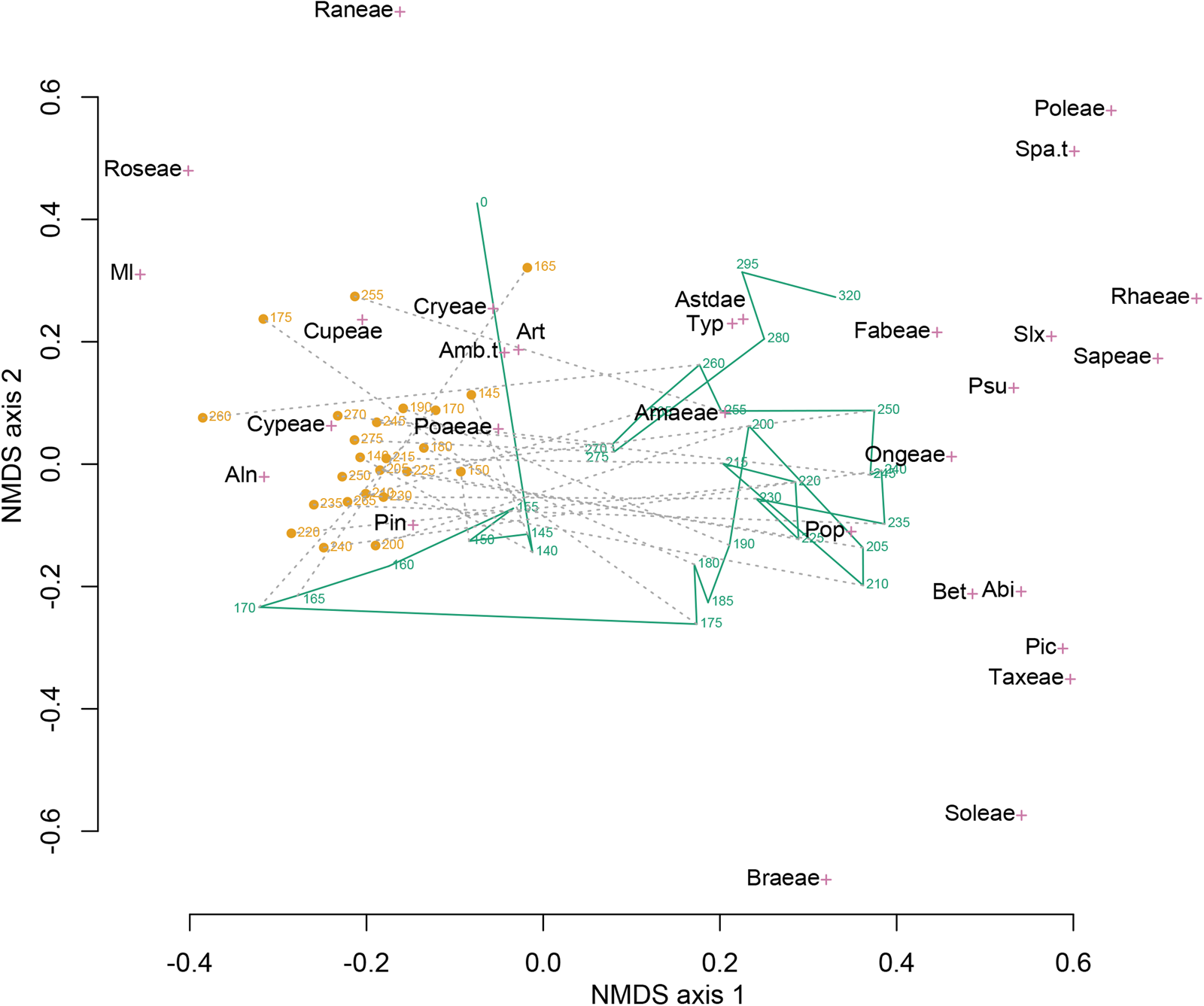
Figure 7. Nonmetric multidimensional scaling (NMDS) of the combined coprolite (orange circles) and sediment (green line) pollen assemblage data set. Sample depths (centimeters below cave floor) are shown for both coprolite and sediment samples. Green line connects sediment pollen samples in stratigraphic order. Gray dashed lines connect coprolite and adjacent sediment samples. The species scores of the 29 pollen taxa are shown by magenta crosses. Abi, Abies; Aln, Alnus; Amaeae, Amaranthaceae; Amb.t, Ambrosia-type; Art, Artemisia; Astdae, Asteroideae; Bet, Betula; Braeae, Brassicaceae; Cryeae, Caryophyllaceae; Cupeae, Cupressaceae; Cypeae, Cyperaceae; Fabeae, Fabaceae; Ml, Pteridophyta (monolete); Ongeae, Onagraceae; Pic, Picea; Pin, Pinus; Poaeae, Poaceae; Poleae, Polemoniaceae; Pop, Populus; Psu, Pseudotsuga; Raneae, Ranunculaceae; Rhaeae, Rhamnaceae; Roseae, Rosaceae; Sapeae, Sapindaceae; Slx, Salix; Soleae, Solanaceae; Spa.t, Sparganium-type; Taxeae, Taxaceae; Typ, Typha. Ninety percent of the variation in differences in pollen assemblages (defined by the chord distance) is explained by the two dimensions of the NMDS ordination.
Examination of pollen-assemblage turnover shows the degree of change of pollen assemblages between adjacent samples for coprolites and sediments and contrasts these changes with differences between coprolites and associated sediments (Fig. 8). We found that the dissimilarity of pollen assemblages between coprolites and associated sediments (chord distance ca. 0.6) was greater than the serial dissimilarity (turnover of pollen assemblages between stratigraphically adjacent samples) within either group (chord distances ca. 0.2–0.4), supporting our first hypothesis. However, we did not find that serial dissimilarity was greater for coprolites than for sediments. Rather, the opposite pattern emerged for most of the P2 zone, thus not supporting the second hypothesis.

Figure 8. Dissimilarity between and within pollen assemblages of coprolites and associated sediment. Dissimilarity is measured by the chord distance. Dissimilarity between coprolites and adjacent sediment (black line) is greater than the turnover (serial dissimilarity) within coprolites or sediments.
Pollen taxonomic richness, estimated by rarefaction to a 175-grain count, was greater in the sediment samples (mean = 11.3) than in the coprolite samples (mean = 10.2). While richness was greater in the sediment than adjacent coprolites for 20 of the 24 analyzed coprolites, a paired t-test showed only marginal significance (t = −1.8, P = 0.08; Fig. 9), thus not fully supporting the third hypothesis.

Figure 9. Pollen taxonomic richness in 24 coprolite samples and 24 adjacent sediment samples estimated by rarefaction on a 175-grain pollen count.
DISCUSSION
Pollen assemblages at Paisley Caves are influenced by the proximal sagebrush steppe, the wetlands of the Chewaucan Basin and lake edge, and the conifers of the forested uplands west of the caves. Adjacent to Paisley Caves, Summer Lake changed in size and salinity throughout the Holocene. Thus, the pollen record should also have been influenced by the changing riparian, lakeshore, and wetland vegetation through time. Surrounding these wetlands, a mix of steppe vegetation, common to the lower elevations of the NGB, graded into juniper woodlands and forest, with sharp community changes occurring within a few hundred meters of elevation, particularly in wetter areas or on north-facing aspects (Wigand and Rhode, Reference Wigand, Rhode, Herschler, Madsen and Currey2002; Grayson, Reference Grayson2011).
The sedimentary pollen analyzed in this study represents more than 7000 yr of deposits that may reflect local climate, hydrology, and Summer Lake's transgressive and regressive shorelines. Our pollen record from cave sediments is similar to the adjacent record developed by Beck et al. (Reference Beck, Bryant and Jenkins2018), with the exception of much higher Abies and Salix pollen percentages in our profile. In contrast, our mammalian coprolite pollen record differs substantially from the adjacent Neotoma coprolite pollen record developed by Beck et al. (Reference Beck, Bryant and Jenkins2020). In the following sections, we discuss the causes of these differences and examine the environmental drivers of the changes in the sediment pollen record in the context of prior studies in the NGB.
P1: Late Pleistocene BA to Holocene
Hudson et al. (Reference Hudson, Hatchett, Quade, Boyle, Bassett, Ali and De los Santos2019, Reference Hudson, Emery-Wetherell, Lubinski, Butler, Grimstead and Jenkins2021) characterize conditions in the Chewaucan Basin during the terminal B-A (ca. 13,000 cal yr BP) as warming with high effective moisture and a deeper lake than immediately prior, with the shoreline only 17 m below and within 100 m horizontally of the base of 5-Mile Point Butte. This time period is poorly represented in the unit 2/6 record with a modeled hiatus (Fig. 6A). As no hiatus exists in other portions of the cave, this hiatus may be due to a localized impact, such as high foot traffic. Our single pollen sample from this time contains a good representation of the riparian and lakeshore taxa of Salix and Typhaceae. In contrast, the high abundance of Artemisia and Ambrosia-type pollen in this zone suggests arid steppe conditions. As is the case today near riparian settings, riparian and arid steppe taxa are closely juxtaposed; our results are consistent with geologic evidence for freshwater being much closer to the caves than it is today. Our findings correspond well with results from other pluvial lake basins near the Chewaucan Basin, including pollen and highwater stand timings from Warner Valley to the east (Wriston and Smith, Reference Wriston and Smith2017) and pollen, macrobotanical analysis, and highwater stand timings from Fort Rock Basin to the north (Friedel, Reference Friedel1993; Egger et al., Reference Egger, Ibarra, Weldon, Langridge, Marion, Hall, Starratt and Rosen2021; McDonough et al., Reference McDonough, Kennedy, Rosencrance, Holcomb, Jenkins and Puseman2022).
The YD is well represented archaeologically through a rich cultural assemblage (Jenkins et al., Reference Jenkins, Davis, Stafford, Campos, Connolly, Cummings, Hofreiter, Graf, Ketron and Waters2013, Reference Jenkins, Davis, Stafford, Connolly, Jones, Rondeau, Cummings, Kornfeld and Huckell2016), but based upon the sediment chronology, there was little sediment material from this time in our sampled Unit 6. This contrasts with Unit 4, where Beck et al. (Reference Beck, Bryant and Jenkins2018) inferred a continuous record through the YD. It is possible that cave habitation and hearths eroded and consumed this layer in Unit 6. The YD is generally described as cool and dry in western North America (Mitchell, Reference Mitchell1976; Allison, Reference Allison1982; Licciardi, Reference Licciardi2001; Vacco et al., Reference Vacco, Clark, Mix, Cheng and Edwards2005; Carlson, Reference Carlson and Elias2013; Jenkins et al., Reference Jenkins, Davis, Stafford, Connolly, Jones, Rondeau, Cummings, Kornfeld and Huckell2016). The YD is characterized in the Summer Lake basin as a period of cooler conditions and increased aridity, ultimately resulting in Summer Lake receding (Cohen et al., Reference Cohen, Palacios-Fest, Negrini, Wigand and Erbes2000; Hudson et al., Reference Hudson, Hatchett, Quade, Boyle, Bassett, Ali and De los Santos2019, Reference Hudson, Emery-Wetherell, Lubinski, Butler, Grimstead and Jenkins2021). After the YD, there was warming and increased effective moisture in conjunction with increasing insolation during Northern Hemisphere summers (Kutzbach et al., Reference Kutzbach, Gallimore, Harrison, Behling, Selin and Laarif1998). While the YD shorelines are poorly constrained at Summer Lake, it appears likely that Summer Lake levels rose at the start of the Holocene (Hudson et al., Reference Hudson, Emery-Wetherell, Lubinski, Butler, Grimstead and Jenkins2021), as has been suggested for nearby Warner Lake (Wriston and Smith, Reference Wriston and Smith2017).
Although truncated by a hiatus, the remainder of zone P1, from 12,100 to 11,100 cal yr BP appears consistent with the YD having been in a period of high aridity. Artemisia and Amaranthaceae pollen increases, and Pinus subg. Pinus decreases. Comparing the relative amounts of the two Asteraceae subgroups, Ambrosia spp. (ragweed) can at times be indicative of highly arid conditions (Thompson, Reference Thompson1996; Dennison-Budak, Reference Dennison-Budak2010), while the Asteroideae-types can be indicative of wetter or cooler conditions (Heusser et al., Reference Heusser, Denton, Hauser, Andersen and Lowell1995; Thompson, Reference Thompson1996; Mudie et al., Reference Mudie, Marret, Aksu, Hiscott and Gillespie2007). Post-YD Ambrosia-type asters are in high abundance until ca. 11,100 cal yr BP, indicative of continuing aridity and increasing temperatures.
Pinus subg. Pinus (representing P. ponderosa and P. contorta) remained fairly low (ca. 20–30%) through P1. Pinus species are highly prolific pollen producers, contributing significantly to the regional pollen signal (Minckley et al., Reference Minckley, Bartlein, Whitlock, Shuman, Williams and Davis2008). While Pinus percentages were higher than the surface sample (Fig. 6A), they were like that of other surface pollen assemblages from Paisley Caves (Beck et al., Reference Beck, Bryant and Jenkins2018) and much lower than Pinus percentages at sites closer to current Pinus population (Beck et al., Reference Beck, Bryant and Jenkins2018, Reference Beck, Bryant and Jenkins2020), supporting the conclusion of Beck et al. (Reference Beck, Bryant and Jenkins2020) that pines were not substantially closer than present to Paisley Caves during this period.
Highly notable is the presence of pollen from Pinus subg. Strobus (<2%) in the P1 pollen assemblage. In the NGB, this pollen type represents Pinus albicaulis (whitebark pine) and Pinus monticola (western white pine). Both species are indicative of higher moisture and lower summer temperatures than those occurring at the basin floor today, as P. albicaulis is found at elevations at or above 2100 m, and P. monticola grows between 1700 and 2000 m. The presence of Pinus subg. Strobus in P1 indicates lower aridity and cooler temperatures at lower elevations during the terminal Pleistocene relative to later periods.
Also notable is the absence of Cupressaceae (J. occidentalis) pollen in P1 samples, indicating either low abundance of Cupressaceae in the basin during P1 or poor pollen preservation within 2/6 sediments. That Cupressaceae was present in the Summer Lake area at this time has been established, as J. occidentalis seeds were recovered from unit 2/6 from both pre- and post-YD deposits (Kennedy, Reference Kennedy2018), and a trace of Cupressaceae pollen during P1 was reported by Beck et al. (Reference Beck, Bryant and Jenkins2018) in a different area of Cave 2. The seeds were recovered primarily from hearth deposits and showed signs of charring (Jenkins et al., Reference Jenkins, Davis, Stafford, Campos, Connolly, Cummings, Hofreiter, Graf, Ketron and Waters2013; Kennedy, Reference Kennedy2018). The presence of Juniperus macrobotanicals within P1 and P2 deposits was likely due to human seed transport to the caves from distances farther than those traveled by rodents and is consistent with what is known about human foraging habits at the time (Grayson, Reference Grayson1993; Longland and Ostoja, Reference Longland and Ostoja2013; Kennedy, Reference Kennedy2018).
P2a: Early Holocene to the eruption of Mount Mazama
P2a covers the period from 11,100 to 7633 cal yr BP. Summer Lake levels were moderately high during the Early Holocene (Hudson et al., Reference Hudson, Hatchett, Quade, Boyle, Bassett, Ali and De los Santos2019, Reference Hudson, Emery-Wetherell, Lubinski, Butler, Grimstead and Jenkins2021), but after 9000 cal yr BP, lake levels receded rapidly. Pollen-based climate reconstruction from other regional sites show that temperature and aridity peaked at ca. 9000 cal yr BP (Mehringer, Reference Mehringer1987; Minckley et al., Reference Minckley, Whitlock and Bartlein2007). However, the Paisley pollen record for P2a shows increased and sustained high Abies pollen (ca. 20%, from 11,000 to 8000 cal yr BP) and periods of elevated Picea and Cyperaceae pollen (>3%), while more arid-adapted taxa (Amaranthaceae and Artemisia) remain steady at ca. 20%.
Abies grandis × concolor (white fir) is currently present on Winter Rim between 1700 and 2000 m. A decrease in temperature and fire episodes would facilitate the expansion of Abies below 1700 m. Abies grandis × concolor is a shade-tolerant species when young and can remain in the understory for many years until a disturbance opens the tree canopy, after which rapid growth can ensue (Lanner, Reference Lanner1984; Howard and Aleksoff, Reference Howard and Aleksoff2000; Arno, Reference Arno2007). Reduced fire frequency would also favor Abies relative to Pinus.
An alternative explanation for the increase in Abies, a pollen grain that is poorly dispersed due to its thick exine (Bagnall, Reference Bagnell1975), is increased westerly flow during the pollen-producing season. Increased westerly flow, due to a deepening low pressure over the NGB, may have more effectively transported Abies pollen the >20 km from its nearest populations located at higher elevations. Changing strength in westerlies has been invoked to explain an increasing occurrence of Tsuga heterophylla (coastal western hemlock) pollen in interior British Columbia between 9000 and 8200 cal yr BP (Spooner et al., Reference Spooner, Barnes, Baltzer, Raeside, Osborn and Mazzucchi2003).
Picea peaks at 9000 cal yr BP during the P2a period. Beck et al. (Reference Beck, Bryant and Jenkins2018) reported very low Abies and Picea pollen percentages from the unit 2/4, and Picea was also reported from higher-elevation sites such as Deadhorse Lake (2200 m elevation) on Gearhart Mountain (2440 m elevation) 30 km south of Paisley (Minckley et al., Reference Minckley, Whitlock and Bartlein2007). It is probable that the Picea pollen at Paisley Caves originated from Gearhart Mountain.
Typhaceae species are associated with marshy, perennially wet areas. Typhaceae counts decreased throughout P2 and remained low after the Mazama eruption. Waning Typhaceae concentrations in the sediments is a clear indicator of Summer Lake recession moving marshy areas further away from the caves. Typha latifolia and Typha angustifolia are both currently present in the Summer Lake basin, but T. latifolia occurs at a far higher abundance. The genus Sparganium has recently been added to the Typhaceae family, with Sparganium euricarpum present in Summer Lake Marsh. While Sparganium pollen is distinct from Typha, we merged it into Typhaceae, as it was only present in the lowermost two samples. Both genera occupy similar wetland habitats, although Sparganium requires deeper water than Typha sp. (Dennis and Halse, Reference Dennis and Halse2008).
P2b: Mazama tephra to mid-Holocene
P2b (7633–5800 cal yr BP) includes sediments from the Mazama tephra unit. The presence of sedimentary pollen and the occurrence of coprolites within the Mazama tephra unit suggest downward percolation of pollen and/or multiple tephra deposition events. In all sediments other than the Mazama unit, the cave sediment is dense and cemented by Neotoma fecal pellets. However, the Mazama tephra is coarse (>1 mm grain size) and loosely consolidated, with no cementation. This would suggest the pollen stratigraphy within the ca. 26-cm-deep tephra units is mixed. However, we also found an abrupt increase of Pinus within the tephra layer, perhaps attributable to Mazama deposition occurring in at least two phases (Buckland et al., Reference Buckland, Cashman, Engwell and Rust2020). In a study of pollen concentration of the Mazama tephra, Mehringer et al. (Reference Mehringer, Arno and Petersen1977) interpreted an increase in Pinus pollen from 10 to 60% as an initial, rapidly deposited tephra layer followed by a second event during the Pinus pollen season. The pattern of pollen in the Paisley Cave Mazama unit is consistent with multiple ash depositions in different seasons (Mehringer, Reference Mehringer1987; Egan et al., Reference Egan, Staff and Blackford2015). However, the coprolite assemblages do not show a similar increase in Pinus as would be expected if the tephra affected the regional vegetation.
The remainder of P2b shows an increase in Cupressaceae, likely indicating an increase in juniper woodland in the middle Holocene, as well as an increase in Abies. Some herbaceous plant types, such as Brassicaceae and Fabaceae, thrived in response to the tephra deposition. Such plants have adaptations to disturbance, including, in the case of Fabaceae, the ability to fix nitrogen from the atmosphere.
Coprolite pollen assemblages
The amount of pollen present within a coprolite reflects seasonality and the natural pollen rain; various dispersal forms, including anemophily (wind dispersed), entomophily (insect dispersed), and zoophily (animal dispersed); the types of plants contributing to ambient pollen; and the amount of pollen output by different plant species (Shillito et al., Reference Shillito, Blong, Green and van Asperen2020). Intake into an organism's mucus system occurs either through passive or intentional ingestion. Passive ingestion occurs through respiration, drinking water with pollen present, eating plant materials with pollen present on the plant surfaces (Wood et al., Reference Wood, Wilmshurst, Wagstaff, Worthy, Rawlence and Cooper2012; Shillito et al., Reference Shillito, Blong, Green and van Asperen2020), or through the predation and consumption of the digestive organs of plant-consuming prey (Carrión et al., Reference Carrión, Riquelme, Navarro and Munuera2001). Pollen has also been intentionally ingested as a food source by Native American people throughout North America, with examples including Typha and Populus pollen used as food seasoning and thickeners, as well as used in cultural customs and rites (Williams-Dean and Bryant, Reference Williams-Dean and Bryant1975; Euler, Reference Euler, D'Azevedo and Sturtevant1986).
Our hypotheses regarding the pollen assemblages of coprolite versus sediment samples were largely supported. First, the dissimilarity between sediment and coprolite pollen assemblages (chord distance between coprolite and associated sediments) was much greater than the serial dissimilarity (chord distance between stratigraphically adjacent samples) within sediments or coprolites (Figs. 7 and 8). This pattern is expected because the sediment pollen assemblage represents a larger area over a longer time, thus capturing regional pollen more consistently. The coprolite assemblage represents a brief temporal window, while the sediment assemblage integrates a decade or more of pollen deposition. Second, the serial turnover among coprolites was not greater than that among sediments. We hypothesized that the sampling of pollen by a foraging human or another large mammal would result in a stochastic pattern from feces “spiked” with variable amounts of pollen in the gut that were inhaled and ingested, while cave sediment pollen represents a much greater spatial and temporal smoothing. However, the turnover in coprolite assemblages was often less than that in sediment samples. Such a pattern might result from a selection of certain pollen types from the environment based on foraging or hunting behaviors. Third, pollen taxonomic diversity was slightly lower in the coprolites than in the sediment samples. This is consistent with sediment samples representing many years of pollen accumulation from a broad regional source, while the coprolite pollen samples only a portion of the landscape and over a brief period of time.
Compared with sediment pollen assemblages, the coprolite pollen has higher abundances of lighter pollen types (Pinus, Cupressaceae, and in P1 and P2b, Artemisia) and wetland pollen types (Cyperaceae, and in P2b, Typhaceae) and lower abundances of heavy pollen types, including Abies, Pseudotsuga, and Amaranthaceae. The higher occurrence of lighter pollen types (e.g., Pinus relative to Abies) in the coprolites than in the sediments is consistent with pollen being inhaled, then moved into the gut by mucus transport. Pollen that remains airborne for longer periods would be more likely to be inhaled. Seasonality may also play a role in the coprolite pollen assemblages. For example, the high abundance of Artemisia in some coprolites may be due to seasonal use of the caves timed with the late-summer flowering of Artemisia. As the production of Pinus and the other regional conifers all occur in the late spring months (Burns and Honkala, Reference Burns and Honkala1990; Osmond et al., Reference Osmond, Hidy and Pitelka1990), we can surmise that there were two seasonal occupational periods of the caves. Further, all of the coprolites examined for this study contained pollen, suggesting no winter occupation of Cave 2.
The higher abundances of wetland taxa, such as Cyperaceae, in coprolites than in sediments is best explained by people and other animals traveling to marsh areas and ingesting pollen in water. The fact that this difference between coprolites and sediments was observed for all time periods suggests that the phenomenon occurred regardless of the distance of the wetlands from the caves. Typha pollen has similar abundance (~0.5–2%) in sediment and coprolites, with the exception of one coprolite with 10% Typha pollen. This particularly high abundance of Typha may be attributable to intentional consumption of Typha pollen, as was practiced by the Native people of the region (Euler, Reference Euler, D'Azevedo and Sturtevant1986).
Cupressaceae (Juniperus) pollen percentages are higher in coprolites than in sediments throughout zones P2a and P2b. This could indicate intentional human or other large mammal interaction with Juniperus woodlands some distance from the caves. This is consistent with human activity at the time, as Juniperus was an important dietary and medicinal resource (Euler, Reference Euler, D'Azevedo and Sturtevant1986; Kennedy, Reference Kennedy2018). This is also consistent with the seasonal timing of Pinus pollination in late spring, as J. occidentalis also begin producing cones in late spring (Miller and Rose, Reference Miller and Rose1995; Adams, Reference Adams2019). An increase in Cupressaceae through the Early Holocene has not been described before in the NGB (Miller and Wigand, Reference Miller and Wigand1994). The increase may represent either an expansion of Juniperus woodlands, the increased use of juniper woodlands by humans or other large mammals, or both.
The Amaranthaceae pollen present in Cave 2 coprolites is likely derived from an alkaline-tolerant Chenopodium. During P1 and P2a, this taxon has low abundance in the coprolites, while in P2b, there is an increased amount relative to the sediments. This change may indicate a change from avoidance of saltbush-dominated playa areas to increased travel through such areas as playas increased in extent through the Early Holocene. The organism that ingested the pollen would have done so in early to midsummer when Atriplex pollen is produced (Hitchcock and Cronquist, Reference Hitchcock and Cronquist2018).
The concentration of pollen in the coprolites varied, with the majority being relatively low pollen concentration, indicative of passive pollen ingestion. There is a major spike in pollen in a coprolite at 200 cm (8800 cal yr BP), matching a spike in sediment pollen concentration at the same depth. The coprolite spike was driven by a high Pinus influx, while the sedimentary spike was the result of high Artemisia and Amaranthaceae pollen, perhaps reflecting a brief cold period. Perhaps the coprolite producer was near Pinus stands, as such places may have provided mesic conditions at a time when Summer Lake was all but desiccated (Cohen et al., Reference Cohen, Palacios-Fest, Negrini, Wigand and Erbes2000; Friedel, Reference Friedel1993; Licciardi, Reference Licciardi2001; Hudson et al., Reference Hudson, Emery-Wetherell, Lubinski, Butler, Grimstead and Jenkins2021).
CONCLUSIONS
The pollen record from Paisley Cave 2 in south-central Oregon is consistent with prior studies showing steppe conditions persisting throughout much of the Northern Great Basin during the Pleistocene and into the Holocene (Mehringer, Reference Mehringer, D'Azevedo and Sturtevant1986). However, differences in climate, the presence of large freshwater lakes, and changes in insolation timing and intensity mean that there are no analogous ecological conditions today for the region.
By contrasting the degree of changes between adjacent pollen sample types, this study found that the dissimilarity of pollen assemblages between coprolites and associated sediments was greater than the serial dissimilarity between stratigraphically adjacent samples within either group. However, serial dissimilarity within types was not greater for coprolites than sediments. The coprolites showed localized pollen assemblages related to mammalian survival strategies within a 1–2 day period, resulting in less taxonomic variability over time than sedimentary pollen.
Survival decision making by the coprolite producers is suggested by the high percentage of aquatic/wetland pollen in the coprolites. As large mammals need to drink water frequently, as do potential prey animals, it is reasonable to assume the water sources would be in relatively closer proximity to the caves. Overall, the coprolite pollen shows a strong seasonal signal, with late spring and late summer equally strong, but there are components of early spring and midsummer as well. If the coprolite producers were present at Paisley Cave in late fall or winter, we would expect very low pollen concentration in the coprolites, which was not the case for any of the coprolite samples.
Taphonomy and careful excavations at Paisley Caves have provided the rare opportunity to analyze two pollen taphonomies from the same location. Rarer still was to have both preserved in a long chronological sequence. Pollen from cave sediments can provide a regional environmental reconstruction over time (White, Reference White2007), but it is by contrasting sediment pollen with chronologically related coprolite pollen that additional angles of ecological interactions related to changing climates and ecosystems can be determined. The results of these types of studies can then be applied to questions regarding diet, health, mobility, and other topics relating to past human or other mammalian behaviors.
Acknowledgments
The completion of this article was made possible through the Rippey Graduate Writing Grant received through the Department of Geography at the University of Oregon. We thank Brianna Rollo, R. P. Cromwell, Pat Luther, Matthew Kale, and Olga Saban-Kaup for their contribution to this research. We thank W.W. Oswald and three anonymous reviewers for their comments on the article.
Conflict of Interest Statement
The authors declare no conflict of interest.


