


Many government programmes exist to encourage food stores to provide healthy foods and to regulate the types of foods and beverages sold(1–4). For example, to improve healthy food access, since 2011 the Healthy Food Financing Initiative has provided grants and loans to food outlets (e.g. grocery stores, farmers’ markets) in low-income communities nationwide(1). The Special Supplemental Nutrition Program for Women, Infants, and Children requires stores that accept its vouchers to stock a variety of healthy foods, and the Supplemental Nutrition Assistance Program requires vendors to sell certain types of food groups to low-income families(Reference DeWeese, Todd and Karpyn2). These policies and programmes are based on a belief that the nutritional quality of diets can be enhanced by increasing the number of stores that sell healthy foods, by improving the healthfulness of foods sold in stores and by encouraging people to purchase healthy options. Numerous researchers have investigated factors related to food purchasing decisions, including the types of food stores commonly visited(Reference Hillier, Smith and Whiteman5,Reference Chrisinger, Kallan and Whiteman6) , the distance between residences and stores(Reference Hillier, Smith and Whiteman5) and the differences in foods purchased across store type(Reference Chrisinger, Kallan and Whiteman6,Reference Volpe, Okrent and Leibtag7) . This research should inform policy making about how to improve spatial access to healthy foods. However, most investigators have focused on the ‘food store component’ (particularly, the spatial access to full-service supermarkets, supercentres and convenience stores) of the larger ‘built environment’ context.
Food purchases are also affected by other built environment factors such as transportation infrastructure, the number of fast-food and sit-down restaurants(Reference Cerin, Frank and Sallis8) and other complementary activity locations such as schools, churches and childcare services(Reference Lovasi, Hutson and Guerra9). In addition, several studies have linked food store type to the nutritional quality of foods purchased. For example, individuals tend to purchase fewer sugar-sweetened beverages and packaged foods in supermarkets than in convenience stores(Reference Stern, Robinson and Ng10,Reference Gustafson11) . Thus, access to transportation and related factors, including street connectivity, the number of parking spaces and access to public transit, may affect which type of store (e.g. full-service supermarkets v. convenience stores) is relatively more convenient(Reference D’Angelo, Suratkar and Song12), and convenience may affect the nutritional quality of foods purchased(Reference Stern, Robinson and Ng10–Reference D’Angelo, Suratkar and Song12).
Among studies focusing on only the food store component, Kyureghian et al. (Reference Kyureghian, Nayga and Bhattacharya13) and Handbury et al. (unpublished results) explicitly assessed the potential access to food stores by looking at large geographic area (∼ 20 km from home). These investigators concluded that, at best, food store density explained only a small fraction of the variation in the nutritional quality of foods purchased. Although people purchased outside their closest supermarket(Reference LeDoux and Vojnovic14,Reference Shannon15) , people were still more likely to use stores closer to home(Reference Hillier, Smith and Whiteman5,Reference Gustafson11,Reference Hillier, Smith and Cannuscio16) even when the regional food market environment matters. In the present paper, we examine both availability of neighbourhood food stores and potential access to food stores in the region. We define ‘neighbourhood’ as a small area that provides for daily needs and convenience to shop for certain types of foods (but not necessarily by foot). We define ‘region’ as an expansive area in which people may combine food purchasing with other needs that must be met by long-distance travel, such as work and entertainment, the area of which may be larger than census-defined places (e.g. city, town and village).
Although prior research identified the effects of transportation and land-use factors (such as walkability and street connectivity), that research focused primarily on characteristics around home(Reference Cerin, Frank and Sallis8,Reference Rose and Richards17) without accounting for regional land-use patterns and accessibility. Regional-scale analysis is important because household shopping activity is far more dispersed rather than concentrated in the immediate neighbourhood around home(Reference Chen and Kwan18). Shopping activity is often combined with other home support activities such as meeting children after school(Reference DiSantis, Hillier and Holaday19,Reference Shannon20) . Much of this research is through qualitative methods and/or limited to few metropolitan areas. The present study is among the first to use a national sample that accounts for all these factors using quantitative metrics. We studied the association between food shopping behaviours and density of neighbourhood supermarkets and convenience stores, the broader built environment context of the neighbourhood (diversity and density of non-food locations, street connectivity) and regional accessibility.
We used data from the Nielsen Homescan Consumer Panel Dataset for 2010(21) on self-reported household expenditures for fruits and vegetables for 22 448 households in 378 metropolitan statistical areas (MSA) in the continental USA. The large national-level data set enabled us to examine geographic and market factors related to food purchasing decisions and to generalize and extrapolate our findings to other areas(Reference Laska, Graham and Moe22). Our work enhances the understanding of factors that influence where and how people purchase foods and, thus, policies to encourage healthy food purchasing should be implemented with the same considerations(Reference Chrisinger, Kallan and Whiteman6). We addressed the following research questions:
1. How do the numbers of neighbourhood supermarkets and convenience stores relate to the purchase of fruits and vegetables?
2. How do other built environment characteristics such as regional destination accessibility, neighbourhood destination diversity, availability of neighbourhood destinations and neighbourhood street connectivity relate to the purchase of fruits and vegetables?
3. How is the relationship between the number of food stores and the purchase of fruits and vegetables affected by including other built environment factors in the analysis?
Methods
Study sample
Nielsen’s National Homescan Consumer Panel Dataset(23) is an ongoing, nationally representative survey of 40 000–60 000 US households; the survey includes food and beverage purchase data(21). We used food purchase data from The Nielsen Company (US), LLC and marketing databases provided by the Kilts Center for Marketing Data Center at The University of Chicago Booth School of Business. Nielsen households (referred to as ‘households’ hereafter) reported food purchases in the following types of retail stores: warehouse clubs, mass merchandisers and supercentres, chain grocery stores, non-chain grocery stores, convenience stores, drug stores, dollar stores, ethnic and specialty stores, and others(Reference Stern, Robinson and Ng10).
We selected 27 422 magnet households from the total of 60 658 households available for 2010 (analysed in 2018). Magnet households are households that reported non-standard Universal Product Code (UPC) products, which included random-weight items such as fruits, vegetables, meats and in-store baked goods(Reference Einav, Leibtag and Nevo24,Reference Zhen, Taylor and Muth25) , in addition to the standard UPC (or branded UPC) products. We focused on magnet households to obtain more information about how people purchase fruits and vegetables because many non-standard fruit and vegetable UPC products are of random weight. The household-level characteristics of magnet households did not differ greatly from the characteristics of non-magnet households (see Supplemental Fig. S1 in online Supplemental Sample).
We excluded 4559 households outside the MSA because individuals in outlying rural areas may commute considerable distances to shop for food; large commuting distances make less reasonable the use of a uniform buffer size (e.g. 5 km) to represent a neighbourhood compared with MSA. We excluded 131 households that lacked covariate information and 284 households that had extremely low or high values of expenditures for both fruits and vegetables (below the 2nd percentile or above the 98th percentile of the expenditures). Our final sample was 22 448 households (see online Supplemental Sample for more details regarding the sample construction).
Measures
We aggregated the purchases of fruits and vegetables in each shopping trip over the entire year of 2010 to partially address potential random purchasing behaviours (i.e. impulsive purchases) in a short observational period (e.g. weekly or monthly) for each household in the sample(Reference DiSantis, Hillier and Holaday19). In total, the households made 418 963 and 700 195 trips to purchase fruits and vegetables and, in turn, recorded 1 198 224 and 1 501 437 expenditures in 2010. Household had an average of 18·7 and 31·2 trips and 53·4 and 66·9 records for fruit and vegetable purchases in 2010. We used expenditure values instead of weight values because magnet households reported expenditures only for non-standard UPC products. We calculated the self-reported expenditures on fruits and vegetables (separately) as the sum of standard UPC products and non-standard UPC products. The correlation between total expenditures at MSA level and the food quantity for UPC products was 0·99 and 0·98 for fruits and vegetables. While Nielsen did not report quantity for non-UPC products, this high correlation suggested that expenditures were a reasonable substitute for quantity in our analyses and our conclusions were not affected by regional variation in food prices.
To address the difficulty of recording expenditures on non-standard UPC products, Nielsen tracks non-standard UPC created by each retailer who assigns them to random-weight products to identify and update food items(Reference Zhen, Taylor and Muth25). Thus, magnet households can either scan the non-standard UPC from a reference card accompanying the Nielsen-provided scanner or choose from a list of products in the mobile application to record product type and total price. Although self-reported random-weight products are particularly susceptible to measurement error, the degree of error in Homescan is comparable to the error in other commonly used economic data sets(Reference Einav, Leibtag and Nevo24). See online Supplemental Measures and Supplemental Table S1 for the details of developing expenditures for fruits and vegetables.
Because Nielsen disclosed only the zip code tabulation area (ZCTA) in which the households resided, we used the centroid of ZCTA as a proxy for the exact residential location of the households. We used food resource data from the 2010 ReferenceUSA data set (University of North Carolina at Chapel Hill)(26). We opted to use ReferenceUSA instead of other food resource data (e.g. Dun & Bradstreet) because of higher accuracy and validity in identifying the type and location of retail food outlets(Reference Fleischhacker, Evenson and Sharkey27,Reference Fleischhacker, Rodriguez and Evenson28) . To reflect the potential food sources near home, we characterized neighbourhood food availability as the number of supermarkets and convenience stores in a 5 km buffer (referred to as ‘neighbourhood’ hereafter) around the centroid of a household’s residential ZCTA. We classified the supermarkets and convenience stores according to the six-digit primary Standard Industrial Classification (SIC) code. Some private data companies such as Infogroup have appended a two- to four-digit extension to the original SIC to update and expand the system for more precise definition of business classification. See Supplemental Table S2 in online Supplemental Measures for the classification of food stores based on the six-digit Infogroup primary SIC code. We cleaned the longitudinal and latitudinal information of the retail food outlet data to maximize their accuracy (e.g. fix incorrect decimal points). We used ArcGIS version 10.5 to calculate the counts of supermarkets and convenience stores in the 5 km buffer.
To measure the regional potential household accessibility to fruits and vegetables, we used regional destination accessibility(Reference Ramsey and Bell29) from the Smart Location Database (SLD)(30). The US Environmental Protection Agency developed SLD to include different indicators for built environment and location efficiency for US Census block groups. The regional destination accessibility measure in SLD was obtained by calculating the number of employees in a 45 min automobile travel time (network travel time decay weighted). This measure captures both the size of opportunities and time travelled, and the measure is routinely used in transportation analyses(Reference Veldhuisen, Timmermans and Kapoen31). To generate the value of the regional destination accessibility for households, we spatially linked the centroid of a household’s residential ZCTA to the SLD block group in which the centroid fell. See online Supplemental Measures for the details of developing regional destination accessibility.
We constructed neighbourhood destination diversity to reflect how the attractiveness of other potential daily or weekly routine destinations may affect food purchase. A diverse neighbourhood may affect fruit and vegetable expenditures by redirecting food purchasing time to other activities, such as eating out(Reference Bernardin, Koppelman and Boyce32). To generate an entropy index of neighbourhood destination diversity in the 5 km buffer, we used the American Time Use Survey 2010, from which we identified three types of destinations visited before or after grocery shopping: (i) other store/mall; (ii) locations for socializing; and (iii) restaurants. See online Supplemental Measures for details on identifying these destinations. We defined other stores/malls as department stores, retail shops and wholesale clubs. Locations where people socialized were churches, health-care services and childcare services. Restaurants were fast-food and sit-down establishments. The entropy equation has been used widely in different land-use entropy formulations(Reference Ramsey and Bell29). The formula we used to calculate neighbourhood destination diversity is as follows:
 $${\rm{Neighbourhood \ destintation \ diversity}} = {{{ - 1}}\over{{\ln (3)}}}\sum\limits_{i = 1}^3 {{p_i}} \cdot \ln \left( {{p_i}} \right),$$
where p i is the proportion of the destinations in category i (i = 1, 2, 3). Entropy ranges from 0 (homogeneity, all destinations in one category) to 1 (heterogeneity, an even mixture of type of destinations). Because the entropy value could not reflect the total size of neighbourhood destinations, we also incorporated the total number of these three types of neighbourhood destinations. We obtained destinations/locations data from the 2010 ReferenceUSA data set and classified destinations/locations according to their six-digit Infogroup primary SIC codes (Supplemental Table S2 in online Supplemental Measures). We used ArcGIS version 10.5 to calculate the count of each type of destination/location in the 5 km buffer.
In addition, we used the SLD measure of neighbourhood street connectivity to reflect the directness of travelling to destinations; the degree of directness may increase the convenience of purchasing fruits and vegetables by decreasing transportation costs. The SLD estimated neighbourhood street connectivity as the total number of street intersections divided by total land area for each census block group. We generated this street connectivity variable by averaging the connectivity values of block groups with centroids in the 5 km buffer (see online Supplemental Measures for the details).
The household-level covariates we used included education level of female head of household (high school or below, college or higher, no female head)(Reference Volpe, Okrent and Leibtag7,Reference Kyureghian, Nayga and Bhattacharya13) , annual household income (<$US 20 000, $US 20 000–59 999, ≥$US 60 000)(Reference Volpe, Okrent and Leibtag7,Reference Kyureghian, Nayga and Bhattacharya13,Reference Weatherspoon, Oehmke and Dembélé33–Reference De Roos, Binacchi and Whybrow35) , race (White, Black, Asian, other)(Reference Kyureghian, Nayga and Bhattacharya13,Reference Weatherspoon, Oehmke and Dembélé33,Reference Volpe and Okrent34) , household size (1, 2, 3, ≥4)(Reference Kyureghian, Nayga and Bhattacharya13,Reference Weatherspoon, Oehmke and Dembélé33) , marital status of household head(s) (married, widowed, divorced/separated, single)(Reference Kyureghian, Nayga and Bhattacharya13), presence of children (yes/no)(Reference De Roos, Binacchi and Whybrow35,Reference Lee, Hickman and Washington36) , number of employees in the household (0, 1, ≥2, household head excluded), and expenditures for vegetables (in the fruit model) and fruits (in the vegetable model). We retrieved all household-level covariates from the Nielsen Homescan Consumer Panel Dataset for 2010 (see online Supplemental Measures for the details). Neighbourhood-level variables, assessed via either the residential census block group or census tract, included the percentage of zero-car households from the SLD and the percentage of households below the poverty line from the 2008–2010 American Community Survey. To obtain the values of percentage of zero-car households and percentage of households below the poverty line, we spatially linked the centroid of a household’s residential ZCTA to the SLD census block group or American Community Survey census tract in which the centroid fell. The area covariate was urbanicity in which the centroid of a household’s residential ZCTA fell, which was classified by the US Census Bureau as urbanized area, urban cluster or non-urban area.
Statistical analyses
We used separate three-level linear mixed-effect regression models for fruits and vegetables. The 22 448 households were nested in 8837 ZCTA in 378 MSA. The median value was 2 (interquartile range (IQR) = 2) for the number of households that resided in the same ZCTA. The number of households in the same ZCTA ranged from one to fifteen. There were 3557 (40·3 %), 1941 (22·0 %), 1286 (14·6 %) and 2053 (23·1 %) ZCTA that had one, two, three and more than three households in the same ZCTA, respectively. We included random intercepts for each ZCTA to enable the responses to vary with the ZCTA in which the households were nested(Reference Feng, Glass and Curriero37) and, similarly, we included random intercepts for each MSA to enable responses to vary with the MSA. The random intercepts may partially account for the regional characteristics such as price variations across MSA. The distribution of household expenditures for fruits and vegetables was right-skewed (median = 99·0 (IQR = 133·4) for fruits; median = 104·2 (IQR = 129·6) for vegetables), so we used the logarithmic transformations of expenditures in the final regression models. The exposure variables were number of neighbourhood supermarkets and convenience stores, regional destination accessibility, neighbourhood destination diversity, availability of neighbourhood destinations, neighbourhood street connectivity, and the other household-, neighbourhood- and area-level covariates. We did not use the Nielsen sampling weight because the initial sample marginal distributions that were used to create the weights were not representative of the sample we retained for our analysis(Reference Kyureghian, Nayga and Bhattacharya13). We performed statistical analyses with R × 64 version 3.5.1 and Rstudio version 1.1456, using the lme4(Reference Bates, Mächler and Bolker38) package to run the linear mixed-effect regression models.
Sensitivity analyses
The centroid of ZCTA may be problematic as a proxy for the real home address, particularly for suburban households in large ZCTA. ZCTA sizes ranged from 0·02 to 5037·5 km2 with a median value of 49·1 km2 (IQR = 108·1 km2). We had 3068 ZCTA (34·7 %) with a land area below 27·1 km2 (the average size of ZCTA in Los Angeles–Long Beach–Anaheim, CA). We had 1006 ZCTA (11·4 %) with a land area equal to or greater than 27·1 and below 41·5 km2 (41·5 km2 was the average in Chicago–Naperville–Elgin, IL–IN–WI). We had 2932 ZCTA (33·2 %) with a land area equal to or greater than 41·5 and below 153·5 km2 (153·5 km2 was the average in Tulsa, OK). Lastly, we had 1831 ZCTA (20·7 %) with a land area equal to or greater than 153·5 km2. To examine the severity of using centroid of ZCTA as a proxy for the real home address, we randomly selected a point from a household’s residential ZCTA to approximate the ‘unknown’ address of all households in the same ZCTA. We used ‘create random point’ tool in ArcGIS version 10.5 and (re)measured the built environmental factors based on these ‘random points’. We compared the results with built environment measures based on ZCTA centroids (see Tables 2 and 3). In addition, we ran the models on the reduced sample (n 17 420 for fruits and n 17 394 for vegetables), excluding households located in 1831 largest ZCTA (with a land area equal to or greater than 153·5 km2). This is because using centroids or randomly selected points as housing residence to measure built environment factors in the 5 km buffer may not be accurate and such problem was particularly severe for large ZCTA.
In addition to the 5 km buffer, we used a 3 km buffer to test the sensitivity of the neighbourhood definition on the results because a recent study indicated that 3 km reflects the distance people travel to neighbourhood convenience stores(Reference Rummo, Meyer and Boone-Heinonen39). In addition, we ran also the models on the reduced sample (between 3rd and 97th percentile of the expenditures) to test the effect of outlier definition (purchasers of few or many fruits or vegetables).
Results
Descriptive statistics
The households in our sample were predominantly White and highly educated; 58·3 % of households had an annual income greater than $US 60 000 (Table 1); the median household income for all the USA was $US 51 144. Approximately 59 % of the households did not have a supermarket in their neighbourhoods. Their log-transformed expenditures for fruits and vegetables (mean = 4·4 for fruits and 4·5 for vegetables) were statistically, but not substantially, different (P = 0·007) from their peers who had one neighbourhood supermarket (mean = 4·5 for fruits and 4·5 for vegetables) or more than one supermarket (mean = 4·5 for fruits and 4·5 for vegetables; data not shown). The median value of the number of neighbourhood convenience stores was 6, with 25th percentile and 75th percentile values of 2 and 16.
Table 1 Sample characteristics of the study households (n 22 448) in the continental USA, 2010
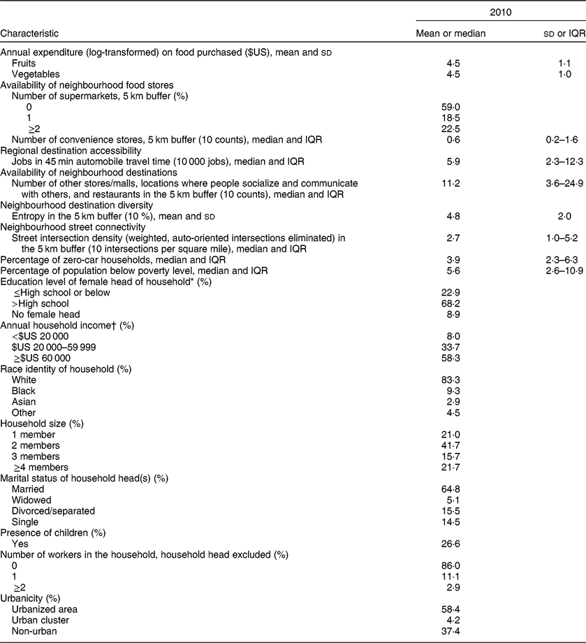
n, number of observations; IQR, interquartile range.
Median and IQR (25th–75th percentile) are presented for continuous variables not normally distributed. Categorical variables are expressed as percentage (%).
Food purchase data and household-level sociodemographic data were derived from the Nielsen Homescan Consumer Dataset in 2010. Copyright © 2018, The Nielsen Company.
* For households with two heads of household, Nielsen designates the characteristics of the head of household as whoever makes most of the purchasing decisions.
† The value represented ranges of total household income for the full year that is 2 years prior to the panel year.
In our sample, on average, households in Beckley, WV had the lowest log-transformed expenditure for fruits (mean = 3·5), whereas Farmington, NM had the highest (mean = 5·6; data not shown). Similarly, Hanford–Corcoran, CA, a metropolitan area in the agricultural San Jaoquin valley, on average, had the highest log-transformed expenditure for vegetables (mean = 5·5), whereas Cape Girardeau–Jackson in MI and IL had the lowest (mean = 3·6). Although there were essentially no differences in the vegetable expenditures among urban and non-urban households, there were marginal differences (P < 0·001) in the fruit expenditures, with households in urban clusters having the lowest average expenditure (mean = 4·4) compared with urbanized areas (mean = 4·5) and non-urban (mean = 4·5).
Regression analyses
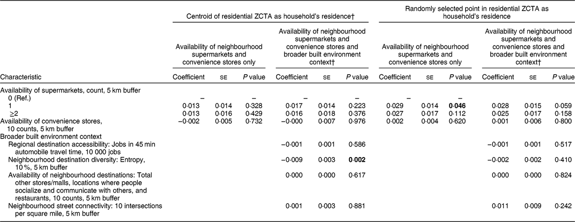
Analyses including only the availability of neighbourhood supermarkets and convenience stores suggested that households in a neighbourhood with at least two supermarkets purchased significantly more (by 4·1 percentage points) fruits than households without a neighbourhood supermarket (Table 2). Controlling for regional destination accessibility, neighbourhood destination diversity, availability of neighbourhood destinations and neighbourhood street connectivity, the differences in expenditures on fruits between households with different numbers of neighbourhood supermarkets were not significant. Households purchased significantly more (2·4 percentage points more) fruits if they lived in neighbourhoods with fewer (10 fewer) convenience stores (Table 2). Households purchased significantly more (0·3 percentage point more) fruits if they lived in neighbourhoods with greater (10 000 jobs more) regional destination accessibility. Households purchased significantly more (1·3 percentage points more) fruits if they lived in neighbourhoods with higher (10 intersections per square mile more) street connectivity. Controlling for the broader built environment context, we did not find a significant difference in expenditures on vegetables among households with different numbers of neighbourhood supermarkets or convenience stores. Controlling for the broader built environment context, we found that households purchased significantly fewer (0·9 percentage point fewer) vegetables if they lived in neighbourhoods with greater (10 percentage points of entropy value greater) destination diversity (Table 3).
Table 2 Cross-sectional associations between annual expenditures (log-transformed) for fruits purchased by Nielsen households (between 2nd and 98th percentile of the fruit expenditures, n 21 710*), availability of neighbourhood (5 km buffer) supermarkets and convenience stores, broader built environment context characteristics, and household-, neighbourhood- and area-level covariates; continental USA, 2010

n, number of observations; ZCTA, zip code tabulation area; Ref., reference category.
Food purchase data and household-level sociodemographic data were derived from the Nielsen Homescan Consumer Dataset in 2010. Copyright © 2018, The Nielsen Company.
P values in bold indicate statistically significant associations (P < 0·05).
* We excluded households who reported extremely low or high values for purchases of fruits and vegetables (both simultaneously), defined here as less than the 2nd percentile or greater than the 98th percentile.
† Regressions controlled for percentage of zero-car households in residential census block group, percentage of population below poverty level in residential census tract, household income, race identity of household, household size, marital status, if there is at least one child in the family, number of employed household members (household head excluded), expenditure (logarithmic-transformed) on vegetables and urbanicity (R × 64 version 3.5.1 and Rstudio version 1.1456).
Table 3 Cross-sectional associations between annual expenditures (log-transformed) for vegetables purchased by Nielsen households (between 2nd and 98th percentile of the vegetable expenditures, n 21 686*), availability of neighbourhood (5 km buffer) supermarkets and convenience stores, broader built environment context characteristics, and household-, neighbourhood- and area-level covariates; continental USA, 2010
n, number of observations; ZCTA, zip code tabulation area; Ref., reference category.
Food purchase data and household-level sociodemographic data were derived from the Nielsen Homescan Consumer Dataset in 2010. Copyright © 2018, The Nielsen Company.
P values in bold indicate statistically significant associations (P < 0·05).
* We excluded who households reported extremely low or high values for purchases of fruits and vegetables (both simultaneously), defined here as less than the 2nd percentile or greater than the 98th percentile.
† Regressions controlled for percentage of zero-car households in residential census block group, percentage of population below poverty level in residential census tract, household income, race identity of household, household size, marital status, if there is at least one child in the family, number of employed household members (household head excluded), expenditure (logarithmic-transformed) on fruits and urbanicity (R × 64 version 3.5.1 and Rstudio version 1.1456).
By controlling for the broader built environment context and also shifting the housing residence from the centroid of household residential ZCTA to a randomly selected point in the same ZCTA, we found that the availability of neighbourhood supermarkets was not associated with the expenditures on fruits or vegetables (Tables 2 and 3). Similarly, after shifting the housing residence, we found that households purchased significantly more (2·4 percentage points) fruits if they lived in neighbourhoods with 10 fewer convenience stores (Table 2). Conversely, after shifting the housing residence, we found that street connectivity (Table 2) and neighbourhood destination diversity (Table 3) were not positively and inversely associated with the expenditures for fruits and vegetables.
Analyses using the reduced sample excluding households from large ZCTA, using the 3 km buffer to proxy neighbourhood and using the outlier-reduced sample (between 3rd and 97th percentile of the expenditures) generated similar results compared with the primary analyses (see Supplemental Tables S3–S8 in online Supplemental Data Analyses and Results).
Discussion
The results point to the evidence of cross-sectional associations between availability of neighbourhood convenience stores, regional destination accessibility, neighbourhood destination diversity, neighbourhood street connectivity and self-reported food purchases. Both the number of convenience stores and the broader built environment context of food stores were important to consider when evaluating the relationship between food stores and healthy food purchasing.
Our findings add to those of some studies that have concluded that the number of neighbourhood supermarkets is not (or only marginally) associated with food purchase(Reference Kyureghian, Nayga and Bhattacharya13,Reference Rahkovsky and Snyder40) . The healthy food purchases of households in neighbourhoods with many supermarkets were only marginally higher than the healthy purchases in neighbourhoods with few supermarkets. However, this marginal effect disappeared when we considered the broader built environment characteristics. In sum, the data indicated that close proximity to supermarkets likely did not motivate food purchasing after taking into account other shopping trip contexts(Reference Minaker, Olstad and Thompson41) such as street network and other food and non-food destinations. Although close to three-fifths of the sample lived in neighbourhoods with no supermarkets, households probably used stores outside the neighbourhood to compensate for inadequate or unsatisfactory shopping environments. One nationally representative study showed that 60 % of households still chose supermarkets as the primary type of food store visited(Reference Hillier, Smith and Whiteman5). Therefore, for advancing food environment research and interventions, it is important to understand why people choose supermarkets outside their neighbourhoods.
The fact that neighbourhood supermarkets were not associated with food purchase likely holds because our sample was skewed towards households with higher than national median income and was predominantly White. These households have fewer barriers to access non-neighbourhood food stores compared with low-income households. However, studies show that low-income households travelled longer/further for food shopping if driving or car-sharing was affordable and available(Reference Rahkovsky and Snyder40,Reference Kerr, Frank and Sallis42) . Therefore, policy interventions should proceed cautiously if they focus exclusively on increasing the availability of supermarkets in a neighbourhood and focus more comprehensively on accessibility.
Households in neighbourhoods with plentiful convenience stores reported purchasing fewer fruits than households in neighbourhoods with relatively fewer convenience stores. While our sample contained only 8 % of households in the lowest income category, the median number of neighbourhood convenience stores was similar for households with different income levels (7, 7 and 6 for groups with annual income of < $US 20 000, $US 20 000–59 999 and ≥ $US 60 000). Therefore, it was unlikely that the inverse association between convenience stores and fruit expenditures was the result of convenience stores targeting poor households or poor households self-selecting to live in neighbourhoods with many convenience stores. Our results agree with a previous study that had balanced representation of age, race, gender and education and which indicated that neighbourhood convenience stores were inversely associated with self-reported diet quality(Reference Rummo, Meyer and Boone-Heinonen39). Everyone, not only individuals with poor access to supermarkets, should be considered in future studies of the effect of many neighbourhood convenience stores on food purchases. Future work should determine whether convenience stores forestall demand for healthy options by offering unhealthy choices. Does living in a neighbourhood with a relatively high availability of convenience stores encourage people to purchase more unhealthy foods (e.g. energy-dense snacks and sweetened beverages), thus decreasing purchases of more plentiful healthy options (e.g. fruits) in distant outlets? Some studies have supported this hypothesis by finding that participants tended to purchase foods with poor nutritional quality in small stores such as a corner store, gas mart, pharmacy and dollar store(Reference Caspi, Lenk and Pelletier43,Reference Kiszko, Cantor and Abrams44) , although the evidence was limited to individual cities or subgroups.
Although including other built environment context factors contributed to understanding the relationship between food stores and food purchase, we found that the magnitude was small for associations between other built environment context and food purchase. When the neighbourhood street connectivity increased one unit (i.e. the number of road intersections increased by 10), the expenditures for fruits increased by 1·3 %. Higher density of intersections reflects a more pedestrian-friendly neighbourhood with more types of destinations. Possibly, residents of these neighbourhoods had potential destinations other than supermarkets and convenience stores. Thus, in our study, it is likely that we did not capture competing stores that sell fruits and vegetables.
With a 10 % increase in the diversity of neighbourhood destinations, expenditures for vegetables decreased by 0·9 %. This association means that people in a low-diversity neighbourhood (e.g. entropy = 0·36) purchased approximately 2·4 % ({[(0·62 – 0·36) × 100]/10} × 0·9 = 2·4) more vegetables than people in a high-diversity neighbourhood (e.g. entropy = 0·62). Possibly, people in neighbourhoods with greater destination diversity tended to more frequently patronize restaurants and coffee shops, thus they purchased less vegetables. We did not find that households purchased more fruits or vegetables if they lived in a neighbourhood with a greater number of other destinations, such as retail shops, churches and restaurants. The total number of destinations differed from neighbourhood destination diversity. The large number of neighbourhood destinations (e.g. restaurants, schools) we observed may have been a cluster of similar resources (e.g. restaurants), but the association with food purchase may have been different if the households lived in a neighbourhood with diverse and dissimilar destinations, for example two retail shops, one restaurant and a church, as compared with a neighbourhood having five restaurants.
A one unit increase of regional destination accessibility (10 000 jobs in 45 min automobile travel time) led to a 0·4 % increase in expenditures for fruits. Our results agree with other findings that food opportunities were linked to other places during weekly or daily routine travels beyond the home neighbourhood(Reference DiSantis, Hillier and Holaday19,Reference Kerr, Frank and Sallis42,Reference Clifton45) . The average numbers of food and non-food opportunities in a 45 min automobile travel time were 55 000 and 408 000 for households in Tulsa, OK and those in Los Angeles–Long Beach–Anaheim, CA. Ceteris paribus, households in high-accessibility regions (e.g. Los Angeles) spent 10·6 % ([(408 000 – 55 000)/10 000] × 0·3 = 10·6) more on fruits than those in low-accessibility regions (e.g. Tulsa). Future work should be conducted to identify the non-food purchase opportunities that are related to food purchase opportunities and to refine our measurement of regional destination accessibility, which may increase its explanatory power on food purchasing behaviours.
More research on the regional variations of purchases in different MSA is needed because the types of food purchased by households are different. For example, the median value of expenditures for fruits and vegetables in Los Angeles–Long Beach–Anaheim, CA (n 558) was $US 150·6 and $US 142·6, compared with $US 102·5 and $US 131·8 for Tulsa, OK (n 83; data not shown). Using the Kruskal–Wallis H test (Stata 14.0), we found that the difference was significant (P < 0·001) in the median value of food expenditures across the two MSA. Eighty-six per cent of households in Los Angeles had at least one supermarket in the 5 km buffer, compared with 30 % in Tulsa. Households in Los Angeles had, on average, 18 convenience stores in the 5 km buffer, compared with 10 in Tulsa. These findings suggest that regional differences, along with local land-use characteristics, may matter for household food choices.
Limitations
We selected only households that reported magnet data, which limited the generalizability of our results to all US households. Our analytic sample was composed of a greater number of middle-income households with a greater average educational attainment than the US national population(Reference Piernas, Ng and Popkin46,Reference Ford, Ng and Popkin47) . We used the centroid of the ZCTA as a proxy for a household’s exact residential location, which meant that households living in the same ZCTA shared the same built environment characteristics. By using either centroids or randomly selected points, we might have missed small-area differences in the food and built environment, particularly for the 20 % of households located in large ZCTA. Our measure of regional destination accessibility may have included destinations unrelated to food purchase. Commercial sources of data for food outlets are error prone; we carefully cleaned and processed the data to increase their quality, yet errors likely remained. We could not examine the alignment of expenditures with the quantity for non-standard UPC products purchased because the data of quantity were unavailable. But since the alignment of expenditures with the quantity for standard UPC products was high across regions, we assumed that the alignment for non-standard UPC product across regions was similarly high and in turn we assumed that consumption could be measured by expenditures rather than quantity. The measure of expenditures for fruits and vegetables might be inaccurate for people who purchase most of these products in non-conventional stores such as farmers’ markets. Because non-conventional outlets typically do not provide itemized receipts, households that procured food at non-conventional stores likely incurred a greater reporting burden(Reference Zhen, Taylor and Muth25).
Conclusions
The availability of neighbourhood supermarkets was not associated with expenditures for fruits or vegetables, but the availability of neighbourhood convenience stores was associated with fruit expenditures when we included broader built environment factors in our analysis. The broader built environment contributed to understanding how people used neighbourhood food stores, but the association was almost nil when we considered broader built environment context factors with food purchase. Interventions that increase the number of neighbourhood supermarkets should proceed cautiously. Households in an area with fewer available convenience stores, less neighbourhood destination diversity, greater regional destination accessibility and greater neighbourhood street connectivity may purchase more fruits or vegetables, but an explanation for this behaviour requires more thorough study.
Acknowledgements
Acknowledgements: Dr Penny Gordon-Larsen and Dr Daniel Rodriguez provided extensive comments on earlier drafts. Dr Hélène Delisle and Dr Kaleab Baye provided editorial advice. Usual disclaimers about remaining errors apply. Financial support: This research received no specific grant from any funding agency in the public, commercial or not-for-profit sectors. The present paper reports researchers’ own analyses calculated (or derived) based in part on data from The Nielsen Company (US), LLC and marketing databases provided through the Nielsen Datasets at the Kilts Center for Marketing Data Center at The University of Chicago Booth School of Business. The conclusions drawn from the Nielsen data are those of the researchers and do not reflect the views of Nielsen. Nielsen is not responsible for, had no role in, and was not involved in analysing and preparing the results reported herein. Conflict of interest: None. Authorship: K.P. had full access to the data and takes responsibility for the integrity of the data and the accuracy of the data analysis. K.P. and N.K. acquired the data. Both authors contributed to the study concept and design. K.P. performed the statistical analysis. K.P. and N.K. analysed and interpreted the data. K.P. drafted the article. N.K. critically revised the article for important intellectual content. Both authors have revised the manuscript critically and approved the final version. Ethics of human subject participation: This manuscript does not contain any individual person’s data in any form.
Supplementary material
To view supplementary material for this article, please visit https://doi.org/10.1017/S1368980019000910


