


1. Introduction
The appearance of surface ripples beneath gusts of wind is an everyday experience on the water, belying a surprisingly intricate chain of events unfolding beneath the surface. There, an accelerating wind-drift layer breeds two instabilities in sequence: first, the surface instability that generates ripples, followed by a subsurface instability whose growth, finite amplitude saturation and destabilization to three-dimensional perturbations ultimately gives way to persistent turbulence in the centimetres-thick wind-drift layer.
This ubiquitous transition-to-turbulence scenario was observed in a series of laboratory experiments reported by Melville, Shear & Veron (Reference Melville, Shear and Veron1998), Veron & Melville (Reference Veron and Melville1999) and Veron & Melville (Reference Veron and Melville2001), who subjected an initially quiescent wave tank to a turbulent airflow rapidly accelerated from rest to a constant airspeed. One of Veron & Melville (Reference Veron and Melville2001) key results is that both the generation of surface ripples and the transition to turbulence are suppressed by surfactant layered on the water surface. The surfactant experiment proves that ripples are intrinsic to the second slow instability implicated in the turbulent transition of the wind-drift layer under typical conditions. This disproves Handler, Smith & Leighton (Reference Handler, Smith and Leighton2001) hypothesis, repeated by Thorpe (Reference Thorpe2004), that the transition to turbulence is convective.
Motivated by Veron & Melville (Reference Veron and Melville2001) experimental results, we propose a wave-averaged model based on the ‘Craik–Leibovich’ (CL) Navier–Stokes equation (Craik & Leibovich Reference Craik and Leibovich1976) for the evolution of wind-drift layers after the appearance of capillary surface ripples. A key feature of the CL equation is that the surface wave field is prescribed rather than predicted prognostically. We focus on a comparison with a new laboratory experiment similar to those reported by Veron & Melville (Reference Veron and Melville2001) and described in § 2. We describe the formulation and predictions of our wave-averaged model, which uses the simplest viable description of the surface ripples and initial state of the wind-drift layer, in § 3. Our results combine a linear instability analysis of the wind-drift layer just after ripple inception with numerical simulations of nonlinear development of the second slow instability from ripple inception to fully developed wind-drift turbulence.
We have two goals: first, we seek a more detailed understanding of the wind-drifted transition to turbulence. Second, we would like to validate the wave-averaged CL equation, which is central to parameterization of ocean surface boundary layer turbulence (see for example D'Asaro et al. Reference D'Asaro, Thomson, Shcherbina, Harcourt, Cronin, Hemer and Fox-Kemper2014; Harcourt Reference Harcourt2015; Reichl & Li Reference Reichl and Li2019). Toward this second goal, we make some progress and find that our CL-based model qualitatively replicates the laboratory measurements – most strikingly during the transition to turbulence depicted in figure 5. Yet we also find our results are sensitive to the parameters of the prescribed ripples which, owing to uncertainty about the evolving, two-dimensional state of the ripples surrounding the transition to turbulence, prevents unambiguous conclusions about CL validity. In § 4, we discuss how this sensitivity suggests that CL is ‘incomplete’ because it does not also predict the response of the wave field to the currents and turbulence beneath.
2. Laboratory experiments of winds rising over calm water
This paper uses an experiment similar to those reported by Melville et al. (Reference Melville, Shear and Veron1998) and Veron & Melville (Reference Veron and Melville2001). The experiments were conducted in the 42 m long, 1 m wide, 1.25 m high wind-wave-current tank at the Air-Sea Interaction Laboratory of the University of Delaware, and used a computer-controlled recirculating wind tunnel to accelerate a turbulent airflow to 10  $\mathrm {m \ s}^{-1}$ over 65 s. The water depth was maintained at 0.71 m and observations were collected at a fetch of 12 m. An artificial wave-absorbing beach dissipated wave energy and eliminated wave reflections at the downwind end of the tank. A schematic of the experimental set-up is shown in figure 1.

Figure 1. Schematic of the wind-wave-current tank at the Air-Sea Interaction Laboratory of the University of Delaware at a fetch of 12 m, showing (a) the along-wind section imaged by LIF and (b) the cross-wind LIF set-up.
2.1. Laser-induced fluorescence observations
The evolution of initially surface-concentrated dye was observed with a laser-induced fluorescence (LIF) system. Images were acquired with a CCD camera (Jai TM4200CL,  $2048 \times 2048$ pixels) equipped with an 85 mm Canon EF lens focused at the air–water interface. Illumination was provided by a thin 3 mm thick laser light sheet generated by a pulsed dual-head Nd-Yag laser (New Wave Research, 120 mJ pulse $^{-1}$, 3–5 ns pulse duration). The laser light sheet illuminated a thin layer of fluorescent dye carefully applied to the water surface prior to each experiment. Observations were conducted with the vertical light sheet in both along-wind and transverse directions. The LIF camera collected images at a 7.2 Hz frame rate and with a field of view of $11.6 \times 11.6$ cm in the along-wind configuration, and $13.9 \times 13.9$ cm in the transverse direction.
2.2. Surface wave observations
The evolution of the surface wave profiles was collected using a separate CCD camera (Jai TM4200CL,  $2048 \times 2048$ pixels) equipped with a 60 mm Nikor lens focused at the air–water interface. This camera made use of the LIF illumination system and was synchronized with the LIF camera. As with the LIF images, surface profiles images were collected in both along-wind and transverse directions with fields of view of $20.1 \times 20.4$ cm and $24.5 \times 25$ cm, respectively. Surface wave elevation profiles were extracted from the images using an edge detection algorithm based on local variations of image intensity gradients and which used kernel convolution to identify the location of the surface in the LIF images (see Buckley & Veron (Reference Buckley and Veron2017) for details).
In addition, the waves were measured using optical wave gauges made of 200 mW continuous wave (CW) green lasers (2 mm beam diameter) and CCD cameras (Jai CV-M2,  $1600 \times 120$ pixels). A single wave gauge was positioned 2 cm upstream of the LIF field of view; the camera was equipped with a 180 mm Nikon lens, which resulted in a 19.4 $\mathrm {\mu }$m per pixel resolution. A double wave gauge with two adjacent lasers, separated by 1.4 cm, was placed 3 cm downstream of the LIF field of view. There, the camera was equipped with a 60 mm Nikon lens which resulted in a 66.4 $\mathrm {\mu }$m per pixel resolution. At both locations, single-point elevation measurements were obtained at 93.6 Hz.
2.3. Thermal marking velocimetry
In addition to LIF, we employed thermal marking velocimetry (TMV), as developed by Veron & Melville (Reference Veron and Melville2001) and Veron, Melville & Lenain (Reference Veron, Melville and Lenain2008), to measure the surface velocity by tracking laser-generated Lagrangian heat markers in the thermal imagery of water surfaces. In the present experiment, infrared images of the surface were captured by a 14-bit,  $640 \times 512$ quantum well photodetector (8.0–9.2 $\mathrm {\mu }$m) forward-looking infrared (FLIR) SC6000 camera operated at a 43.2 Hz frame rate, with an integration time of 10 ms, and a stated root-mean-square (r.m.s.) noise level below 35 mK. After image correction to account for the slightly off-vertical viewing angle of the imager, the resulting image sizes were $24.6 \times 24.6$ cm.
The infrared imager is sensitive enough to detect minute, turbulent temperature variations in the surface thermal skin layer (Jessup, Zappa & Yeh Reference Jessup, Zappa and Yeh1997; Veron & Melville Reference Veron and Melville2001; Zappa, Asher & Jessup Reference Zappa, Asher and Jessup2001; Sutherland & Melville Reference Sutherland and Melville2013). It thus easily detects active weakly heated markers, generated by a 60 W air-cooled  $\mathrm {CO}_2$ laser (Synrad Firestar T60) equipped with an industrial marking head (Synrad FH Index) and two servo-controlled scanning mirrors programmed to lay down a pattern of 16 spots with 0.8 cm diameter and at a frequency of 1.8 Hz.
The spatially averaged surface velocity was estimated by tracking the geometric centroid of these Lagrangian heat markers for approximately 1 s. Both Gaussian interpolation (which has sub-pixel resolution due to the Gaussian pattern of the laser beam) and a standard cross-correlation technique yielded similar estimates for the surface velocity.
2.4. Summary of experimental results
Figure 2 summarizes the experimental results. Figure 2(a) shows a time series of the characteristic along-wind wave steepness (Melville et al. Reference Melville, Shear and Veron1998),
 \begin{equation} \tilde \epsilon(t) \equiv \sqrt{2 \overline{\eta_x^2}} , \end{equation}
where  $\eta (x, t)$ is the surface displacement measured by the surface imaging camera, $\eta _x(x, t)$ is the $x$-derivative of $\eta$ and the overline $\overline {({\cdot })}$ denotes an $x$ average over the along-wind field of view of the surface imaging camera. Figure 2(b) shows the measured average along-wind surface velocity using TMV. The thick grey line in figure 2(b) plots $A t$, where $A = 1 \ \mathrm {cm \ s}^{-2}$, showing that the surface current increases linearly, at least initially. (The time axis for laboratory measurements is adjusted to meet this line, which constitutes a definition of ‘ $t = 0$’.) Following Veron & Melville (Reference Veron and Melville2001), figure 2(a,b) divides the development of the waves and currents into four stages:
(i) Viscous acceleration, $t=0$–$16$ s. In the first stage, viscous stress between the accelerating wind and water accelerates a shallow, laminar viscous wind-drift layer.
(ii) Wave-catalysed ‘Langmuir’ shear instability,
$t=16$–$18$ s. At $t \approx 16$ s, detectable capillary ripples appear. A wave-catalysed shear instability – which obey the same dynamics as ‘Langmuir circulation’, which often refers to much larger-scale motions in the ocean surface boundary layer (Craik & Leibovich Reference Craik and Leibovich1976) – immediately starts to develop and grow in the wind-drift layer.(iii) Self-sharpening,
$t=18$–$20$ s. When the shear instability reaches finite amplitude, nonlinear amplification due to perturbation self-advection sharpens the instability features into narrow jets and downwelling plumes.(iv) Langmuir turbulence,
$t > 20$ s. The self-sharpened circulations develop significant three-dimensional characteristics and transition to fully developed Langmuir turbulence.


Figure 2. Summary of laboratory measurements: (a) an estimate of the characteristic along-wind steepness of the surface wave field defined in (2.1) from the surface wave profile measurements; (b) the average along-wind surface velocity measured with the TMV technique.
3. A wave-averaged model for the transition to turbulence in wind-drift layers
The main purpose of this paper is to build a model for the four-stage evolution of the wind-drift layer in the water, focusing on the dynamics after the inception of surface capillary ripples.
3.1. Viscous acceleration
As the wind starts to accelerate, viscous stress across the air–water interface drives a laminar wind-drift current in the water. The thick grey line in figure 2 indicates that the average velocity at the water surface nearly obeys
 \begin{equation} U(z=0, t) \equiv U_0(t) = A t, \end{equation}
where  $A \approx 1 \ \mathrm {cm \ s}^{-2}$ and U is the horizontally averaged velocity in the along-wind direction. Veron & Melville (Reference Veron and Melville2001) point out that the viscous stress consistent with linear surface current acceleration is
 \begin{equation} \boldsymbol{\tau}(t) = \alpha \sqrt{t} \hat{\boldsymbol x}, \end{equation}
where  $\boldsymbol {\tau }$ is the downwards kinematic stress across the air–water interface, $\hat {\boldsymbol x}$ is the along-wind direction ( $\,\hat {\boldsymbol y}$ and $\hat {\boldsymbol z}$ are the cross-wind and vertical directions) and $\alpha \approx 0.12\ \mathrm{cm}^2 \ {\rm s}^{-5/2}$ produces $A = \alpha \sqrt {4 / {\rm \pi}\nu } \approx 1\ \mathrm{cm\ s}^{-2}$ given the kinematic viscosity of water, $\nu = 0.011 \ \mathrm {cm}^2 \ {\rm s}^{-1}$. The laminar, viscous wind-drift shear layer in the water forced by (3.2) takes the form (Veron & Melville Reference Veron and Melville2001)
 \begin{align} U(z, t) = U_0(t) \left [ ( 1 + \delta^2 ) \mathrm{erfc} \left ( - \frac{\sqrt{2}}{2} \delta \right ) + \delta \sqrt{\frac{2}{\rm \pi}} \exp \left ( - \frac{1}{2} \delta^2 \right ) \right ] , \quad \text{where } \delta \equiv \frac{z}{\sqrt{2 \nu t}} . \end{align}
Viscous acceleration continues until gravity–capillary ripples appear at the air–water interface when  $t \approx \tilde t \equiv 16$ s and thus $U_0(t) \approx \tilde U_0 \equiv 16\ \mathrm{cm\ s}^{-1}$.
3.2. Instability of the wind-drift layer catalysed by incipient capillary ripples
As soon as ripples appear on the water surface, a second, slower, non-propagating instability begins to grow within the wind-drift layer in the water. Remarkably, this second instability is catalysed by and therefore requires the presence of capillary ripples; for example, Veron & Melville (Reference Veron and Melville2001) show that instability and turbulence are suppressed if ripple generation is inhibited by the presence of surfactant that increases the surface tension.
To describe the development of the wind-drift layer modified by the appearance of capillary ripples, we use the wave-averaged CL Navier–Stokes equation. In the CL equation, the surface wave field is prescribed, which means that wave generation cannot be described. The formal validity of the CL equation requires that the ripples are not too steep. Figure 2(a) plots an estimate of the characteristic wave steepness  $\tilde \epsilon (t)$ defined by (2.1), showing that, by the time ripples reach detectable amplitudes, they have small slopes with $\tilde \epsilon = 0.1$. We thus expect that the CL momentum equation can at least describe the initial development of the instability that follows ripple inception.
The wave-averaged CL equation (Craik & Leibovich Reference Craik and Leibovich1976) formulated in terms of the Lagrangian-mean momentum  $\boldsymbol {u}^{L}$ of the wind-drift layer is
 \begin{equation} \boldsymbol{u}^{L}_t + ( \boldsymbol{u}^{L} \boldsymbol{\cdot} \boldsymbol{\nabla} ) \boldsymbol{u}^{L} - ( \boldsymbol{\nabla} \times \boldsymbol{u}^{S} ) \times \boldsymbol{u}^{L} + \boldsymbol{\nabla} p^{E} = \nu \triangle \boldsymbol{u}^{L} - \nu \triangle \boldsymbol{u}^{S} + \boldsymbol{u}^{S}_t , \end{equation}
where  $\boldsymbol {u}^{S}$ is the Stokes drift of the field of capillary ripples and $p^{E}$ is the Eulerian-mean pressure. The asymptotic derivation of the CL equation (3.4) requires $\epsilon \ll 1$. We require $\boldsymbol {u}^{L}$ to be divergence free (Vanneste & Young Reference Vanneste and Young2022)
 \begin{equation} \boldsymbol{\nabla} \boldsymbol{\cdot} \boldsymbol{u}^{L} = 0 . \end{equation}
The Stokes drift associated with monochromatic capillary ripples propagating in the along-wind direction  $\hat {\boldsymbol x}$ is
 \begin{equation} \boldsymbol{u}^{S}(z, t) = \mathrm{e}^{2 k z} \epsilon^2 c(k) \hat{\boldsymbol x} , \quad \text{where } c(k) = \sqrt{\frac{g}{k} + \gamma k}, \end{equation}
is the phase speed of gravity–capillary waves in deep water with wavenumber  $k$, gravitational acceleration $g = 9.81 \ \mathrm {m \ s}^{-2}$ and surface tension $\gamma = 7.2 \times 10^{-5} \ \mathrm {m}^3 \ {\rm s}^{-2}$. In (3.6), $\epsilon \equiv a k$ is the steepness of the capillary ripples, which is equivalent to $\tilde \epsilon$ in (2.1) for monochromatic waves. In all cases considered here, the Stokes drift (3.6) is minuscule compared with the mean current $\boldsymbol {u}^{L} \sim U$.
We next investigate the stability of the wind-drift layer after ripples are generated. For this, we expand the total velocity around the steady shear flow  $\tilde U(z)$, such that
 \begin{equation} \boldsymbol{u}^{L}(\kern0.7pt y, z, t) = \tilde U(z) \hat{\boldsymbol x} + \boldsymbol{u}(\kern0.7pt y, z, t) , \end{equation}
where  $\tilde U(z) \equiv U(z, \tilde t)$ represents the wind-drift profile ‘frozen’ at $\tilde t = 16$ s, and $\boldsymbol {u} = (u, v, w)$ is the perturbation velocity. Inserting (3.7) into (3.4) and (3.5), introducing a streamfunction $\psi$ with the convention $(v, w) = (-\psi _z, \psi _y)$ and neglecting terms that depend only on the mean flow $U$ or $u^S$ yields the two-dimensional system
 $$\begin{gather} u_t + J(\psi, u) + \varOmega \psi_y = \nu \triangle u , \end{gather}$$
 $$\begin{gather}\triangle \psi_t + J(\psi, \triangle \psi) + u^{S}_z u_y = \nu \triangle^2 \psi , \end{gather}$$
where  $\triangle \psi = w_y - v_z$ is the $x$-component of the perturbation vorticity, $J(a, b) = a_y b_z - a_z b_y$ is the Jacobian operator and $\varOmega = \tilde U_z - u^{S}_z$ is the Eulerian-mean shear – or, as we prefer, the mean total cross-wind vorticity $\boldsymbol {\nabla } \times ( \tilde U \hat {\boldsymbol x} - \boldsymbol {u}^{S} ) = \varOmega \hat {\boldsymbol y}$. Equations (3.8) and (3.9) model the two-dimensional evolution of the wind-drift layer starting just after ripple generation up to the transition to three-dimensional turbulence.
We use the power method (see for example Constantinou Reference Constantinou2015) to extract the fastest growing linear modes of (3.8) and (3.9) by iteratively integrating the wave-averaged equations (3.4) and (3.5) given the decomposition in (3.7) numerically from  $t=\tilde t$ to $t = \tilde t + {\rm \Delta} t$ to obtain $\boldsymbol {u}$. The numerical integrations use Oceananigans (see Ramadhan et al. Reference Ramadhan, Wagner, Hill, Campin, Churavy, Besard, Souza, Edelman, Ferrari and Marshall2020 and Wagner et al. Reference Wagner, Chini, Ramadhan, Gallet and Ferrari2021) with a second-order staggered volume method in a two-dimensional domain. We use two $y$-periodic, vertically bounded domains with dimensions $10 \times 5~\mathrm{cm}$ and $40 \times 5 \ \mathrm {cm}$ to test the dependence of the results on the domain width. Because (3.4) and (3.5) are averaged over surface waves, the domain contains water only and has a flat, rigid top and bottom boundary; surface waves enter the dynamics solely through the prescribed Stokes drift $\boldsymbol {u}^{S}$. Impenetrable, free-slip boundary conditions are applied at the rigid top and bottom boundaries. We use $768 \times 512$ finite volume cells in both domains, with 0.13 mm and 0.52 mm regular spacing in the horizontal and variable spacing in $z$ with minimum vertical spacing $\min ( {\rm \Delta} z ) \approx 0.26 \ \mathrm {mm}$
The initial condition for the  $k$th iteration, $\boldsymbol {u}^k(\kern0.7pt y, z, \tilde t)$, is derived by downscaling the previous iteration evaluated at $\tilde t + {\rm \Delta} t$
 \begin{equation} \boldsymbol{u}^k |_{t = \tilde t} = \left[ \boldsymbol{u}^{k-1} \sqrt{\frac{\tilde E}{E^{k-1}}}\, \right]_{t = \tilde t + {\rm \Delta} t} , \quad \text{where } E^k \equiv \left\langle \frac{1}{2} | \boldsymbol{u}^k |^2 \right\rangle , \end{equation}
and  $\tilde E$ is the prescribed initial kinetic energy at $t = \tilde t$, and $\langle {\cdot } \rangle$ denotes a volume average. The growth rate is estimated for iterate $k$ by assuming that $\boldsymbol {u}^k \propto \mathrm {e}^{s t}$, which implies that $| \boldsymbol {u}^k |^2 \propto \mathrm {e}^{2 s t}$ and
 \begin{equation} s = \frac{1}{2 {\rm \Delta} t} \log \left( \frac{E^k |_{t=\tilde t + {\rm \Delta} t}}{E^k |_{t = \tilde t}} \right). \end{equation}
To apply the power method, we choose the integration window  ${\rm \Delta} t = 0.05~\mathrm{s}$ with an initial perturbation kinetic energy $\tilde E = 10^{-10}\ \mathrm {m}^2\ {\rm s}^{-2}$. We iterate until the growth rate estimate converges by requiring that $(s^k - s^{k-1}) / s^k < 2 \times 10^{-6}$.
Figure 3 shows the structure of the most unstable mode for  $\epsilon = 0.1$ in a $10 \times 5 \ \mathrm {cm}$ domain in $y, z$. Figure 4 shows the results of a parameter sweep from $\epsilon = 0.04$ to $\epsilon = 0.3$, illustrating that the wind-drift layer is susceptible to Langmuir instability for even miniscule ripple amplitudes. Figure 4(a) shows additionally that the growth rate $s$ is linear in wave steepness $\epsilon$, except at the very smallest wave amplitudes, which due to very slow growth rates are probably affected by viscous stress. Note that, in the absence of waves, or alternatively for $\epsilon = 0$, we recover Veron & Melville (Reference Veron and Melville2001) experimental result that instability does not occur at $\tilde t = 16$ s (or any other time within the duration of the experiment). Figures 4(b) and 4(c) show that larger wave steepnesses are associated with smaller instability wavelengths.

Figure 3. Numerically computed structure of the most unstable mode of the wind-drift layer at  $\tilde t = 16$ s ( just after the inception of surface ripples) for surface ripples modelled as gravity–capillary waves with steepness $\epsilon = ak = 0.1$ and wavenumber $k = 2{\rm \pi}/3\ \mathrm{cm}$ in a $10 \times 5$ cm domain in $(\kern0.7pt y, z)$. (a) Structure of the cross-wind perturbation $v'(\kern0.7pt y, z)$ for wave steepness $\epsilon = 0.1$ in a $10 \times 5$ cm domain in $(\kern0.7pt y, z)$, (b) root-mean-square ( $y$-averaged) perturbation profiles.

Figure 4. (a) Growth rate, (b) growth time scale (inverse of the growth rate) and (c) wavelength of the most unstable mode of a wave-catalysed instability of the wind-drift layer ‘frozen’ at  $\tilde t = 16$ s calculated using the power method (see for example Constantinou Reference Constantinou2015) in two domains 10 and 40 cm wide.
We emphasize that the kinetic energy source for growing perturbations is the mean shear  $\tilde U(z)$ and there is no energy exchange between perturbations and the surface wave field within the context of the wave-averaged equations (3.4) and (3.5). To see this, consider that (3.4) and (3.5) conserve total kinetic energy $\int \tfrac {1}{2} | \boldsymbol {u}^{L} |^2 \, \mathrm {d} V$ when $\nu =0$ and $\partial _t \boldsymbol {u}^{S} = 0$ (the effect of viscous stress is negligible during the instability growth for all but the smallest wave amplitudes). This is why we characterize the shear instability as ‘wave catalysed’; while the presence of waves is necessary for instability, and while the instability growth rate is strongly affected by wave amplitude, the kinetic energy of the growing perturbation is derived solely from the mean shear.
3.3. Self-sharpening circulations with jets and plumes
When the wave-catalysed shear instability reaches finite amplitude, it begins to self-sharpen, producing narrow along-wind jets and downwelling plumes. The sharpening – but still two-dimensional – plumes then transport a measurable amount of mean momentum downwards before becoming unstable to three-dimensional perturbations and thereby transitioning to fully developed turbulence. This nonlinear sharpening and depletion of the average near-surface momentum occurs between 17.5 and 20 s, as evidenced by the red shaded region in figure 2(b).
To simulate the second wave-catalysed instability through finite amplitude and toward transition to turbulence, we propose a simplified model based on the wave-averaged equations (3.4) and (3.5) with two main components representing (i) the capillary ripples and (ii) the initial condition at  $\tilde t = 16$ s. We model the evolving capillary ripples as steady, monochromatic surface waves with wavenumber $k = 2{\rm \pi} / 3 \ \mathrm {cm}^{-1}$. We model the condition of the wave tank at $t = 16$ s with
 \begin{equation} \boldsymbol{u}^{L} |_{t=\tilde t} = \tilde U(z) \hat{\boldsymbol x} + \mathbb{U}' \boldsymbol{\varXi}(x, y, z) , \end{equation}
where  $\mathbb {U}'$ is an initial noise amplitude and $\boldsymbol {\varXi }$ is a divergence-free vector whose components are normally distributed random numbers with zero mean and unit variance.
Through experimentation, we find that the instability and transition to turbulence are only weakly sensitive to the wavenumber  $k$. The tuning parameters of our model are therefore (i) the amplitude of the initial perturbation $\mathbb {U}'$, and (ii) the wave steepness $\epsilon$.
We also simulate the evolution of dye concentration  $\theta$ via
 \begin{equation} \theta_t + \boldsymbol{u}^{L} \boldsymbol{\cdot} \boldsymbol{\nabla} \theta = \kappa \triangle \theta , \end{equation}
with molecular diffusivity  $\kappa = 10^{-7} \mathrm {m}^2 \ {\rm s}^{-1}$, the smallest we can reasonably afford computationally. (The correspondence between $\theta$ and rhodamine is imperfect because the molecular diffusivity of rhodamine is $\kappa = 10^{-9} \ \mathrm {m}^2\ {\rm s}^{-1}$.) We initialize $\theta$ with a $\delta$-function at the surface.
We integrate the wave-averaged evolution of the wind-drift layer by solving (3.4) and (3.5) and (3.13) given (3.6) using Oceananigans in a three-dimensional, horizontally periodic, vertically bounded  $10 \times 10 \times 5$ cm domain in $(x, y, z)$ with 0.13 mm regular spacing in $x, y$ and variable spacing in $z$ with $\min ({\rm \Delta} z) \approx 0.26 \ \mathrm {mm}$, corresponding to $768 \times 768 \times 512$ finite volume cells. As discussed above, (3.4) and (3.5) are averaged over surface waves and surface waves enter the dynamics through $\boldsymbol {u}^{S}$. Because the along-wind $x$-direction is periodic, our simulations neglect large-scale along-wind variation in the ripple field and wind-drift layer. We impose the stress (3.2) on $\boldsymbol {u}^{L}$ at the surface and use free-slip conditions at the bottom.
The results of a numerical solution using the wave steepness  $\epsilon = 0.11$ and the initial perturbation amplitude $\mathbb {U} = 5\ \mathrm{cm \ s}^{-1}$ are compared with laboratory measurements in figure 5. (Note that with $\mathbb {U} = 5 \ \mathrm {cm \ s}^{-1}$, the random component of the initial condition hardly counts as a ‘perturbation’. We discuss the significance of this shortly.) Figure 5(a) compares the average surface velocity diagnosed from the simulation with the laboratory measurements presented in figure 2(b). Figure 5(b) plots the maximum absolute vertical velocity, $\max |w^L|$. Figure 5(c–l) compares the simulated dye concentration on
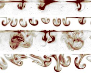
  $(\kern0.7pt y, z)$ slices with LIF measurements of rhodamine from the laboratory experiment, showing how the simulations qualitatively capture the observed formation, evolution and eventual disintegration of coherent structures during the transition to turbulence. Visualizations are shown at $t=18.1$, 19.3, 20.0, 20.7 and 21.7 s. At $t = 18.1$ s (figure 5c,d), the sharpened plumes have only just started advect appreciable amounts of dye. At $t = 19.3$ s (figure 5e,f), the plumes are beginning to roll up into two-dimensional mushroom-like structures. (Note the small, unexplained discrepancy between simulated and measured average surface velocities around $18.1 \ \mathrm {s} < t < 19.3$ s.) At $t = 20.0$ s and $t = 20.7$ s (figure 5g–j) three-dimensionalization and transition to turbulence are underway. At $t = 21.7$ s both the simulated and measured dye concentrations appear to be mixed by three-dimensional turbulence.

Figure 5. (a) Maximum horizontal velocity  $u$. The grey dots are from the laboratory experiments while the blue line shows the numerical experiments. (b) Vertical velocity. (c–l) Evolution of the wind-drift layer after the emergence of capillary ripples.
Figure 6 illustrates the sensitivity of the wave-averaged model to the amplitude of the specified surface ripples and to the amplitude of the random initial perturbation. Figures 6(a) and 6(b) plot the surface-averaged along-wind velocity  $u$ and maximum vertical velocity $w$ for three wave amplitudes $\epsilon = 0.10, 0.11, 0.12$ and for two initial perturbation amplitudes $\mathbb {U}'=2$ and $5 \ \mathrm {cm \ s}^{-1}$. The dependence of the maximum vertical velocity is the most evocative; doubling the initial perturbation shortens the self-sharpening phase (in which the maximum vertical velocity in figure 6(b) flattens before increasing sharply during the transition to turbulence) by a factor of five. Of the four cases plotted in figure 6, only $\epsilon = 0.11$ and $\mathbb {U}' = 5\ \mathrm{cm \ s}^{-1}$ yield the satisfying agreement depicted in figure 5.

Figure 6. Sensitivity of (a) surface-averaged along-wind velocity  $u$ and (b) maximum vertical velocity to the specification of the surface wave field and initial perturbations.
3.4. Langmuir turbulence
Following three-dimensionalization, momentum and dye are rapidly mixed to depth. Figure 7 visualizes (a) the  $x$-momentum and (b) dye concentration at $t=23.4$ s, showing how the flow is organized into narrow along-wind streaks and broader downwelling regions – classic characteristics of Langmuir turbulence (Sullivan & McWilliams Reference Sullivan and McWilliams2010).

Figure 7. (a) Simulated  $x$-momentum and (b) dye concentration at $t = 23.4$ s, showing the streaks and jets that characterize Langmuir turbulence.
In figure 8, we compare the rate which dye is mixed with depth in the simulations vs measured by LIF in the laboratory. Figure 8(a) shows the simulated horizontally averaged tracer concentration in the depth–time  $(z, t)$ plane, while figure 8(b) shows a corresponding laboratory measurements extracted from LIF measurements in the $(\kern0.7pt y, z)$-plane. In figure 8(a,b), a light blue line shows the height $z_{99}(t)$ defined as the level above which 99 % of the simulated tracer concentration resides
 \begin{equation} \int_{z_{99}(t)}^0 \theta \, \mathrm{d} z = 0.99 \int_{{-}H}^0 \theta \, \mathrm{d} z . \end{equation}
Using  $z_{99}(t)$ to compare the tracer mixing rates exhibited in figure 8(a,b), we conclude that the simulations provided a qualitatively accurate prediction of dye mixing rates. If anything, the simulation overpredicts the dye mixing rate – but the data probably do not warrant more than broad qualitative conclusions.

Figure 8. Visualization of mixing rates during measured and simulated wave-catalysed instability via depth–time  $(z, t)$ diagrams horizontally averaged in (a) simulations and (b) LIF measurements. The blue lines denotes the depth above which 99 % of the simulated dye resides; (b) suggests that the simulations overpredict dye mixing rates.
4. Discussion
This paper describes a wave-averaged model for the evolution of wind-drift layers following the inception of capillary ripples. The wave-averaged model predicts that, following ripple inception, the wind-drift layer is immediately susceptible to the growth of a second, slower ‘wave-catalysed’ instability. Wave-averaged simulations show that the evolution of the wave-catalysed instability from initial growth through transition to turbulence is sensitive not only to the amplitude of the surface ripples, but also to the amplitude of the substantial perturbations required both to seed the growth of the second instability and to destabilize initially two-dimensional jets and plumes during the transition to turbulence.
We model the seeding and destabilizing perturbations as random velocity fluctuations imposed at the time of ripple inception. However, in wind-drift layers in the laboratory or natural world, perturbations may be continuously introduced both by turbulent pressure fluctuations in the air and, perhaps more importantly, by inhomogeneities in the ripple field (see figures 3 and 15 in Veron & Melville Reference Veron and Melville2001). We hypothesize that the substantial amplitude of the initial perturbations required in our simulations compensates for this missing physics.
One of the original goals of this work was to probe the potential weaknesses of the wave-averaged CL equation, which is widely used for process studies and parameterization of ocean surface boundary layer turbulence (Sullivan & McWilliams Reference Sullivan and McWilliams2010). For this, we use a comparison between numerical simulations of the CL equations and the controlled, well-characterized laboratory experiments described by Veron & Melville (Reference Veron and Melville2001). Of particular concern are two potentially restrictive assumptions required to derive the CL equation: (i) the surface wave field must be nearly linear; and (ii) characteristic time scales associated with the flow beneath the waves are much longer than the time scale of the waves. The wind-drift layer transition to turbulence is particularly useful for validation; while the two assumptions are comfortably justified at first, they are eventually violated as both the flow and surface ripple field become more nonlinear.
We find that CL-based model is successful – in a sense. For example, figure 5 shows that, for an appropriate initial perturbation and a wave field amplitude, the timing, characteristic scales, finite-amplitude development and breakdown into three-dimensional turbulence are well simulated. Yet, despite this qualitative success, firm conclusions about CL validity prove elusive due to the strong sensitivity of our results to ripple amplitude – which is evolving and two-dimensional in the laboratory experiments rather than uniform and steady, as in our model. In particular, figure 6 shows that changes of 10 % in the amplitude of the constant surface waves prescribed in our CL-based model are sufficient to degrade the accuracy of the simulated instability. This sensitivity, together with Veron & Melville (Reference Veron and Melville2001) observations that the measured ripple field is refracted and organized by turbulence in the wind-drift layer, suggests that two-way wave–turbulence coupling is important and should be described in a ‘predictive’ theory for turbulent boundary layers affected by surface waves. Further progress requires not just theoretical advances to couple wave evolution with the CL equations, but also experiments that obtain more precise two-dimensional measurements of the evolution of the capillary ripples.
Acknowledgements
We acknowledge stimulating discussions with B. Young and N. Constantinou and helpful comments from three referees and the editor.
Funding
G.L.W.'s work is supported by the generosity of Eric and Wendy Schmidt by recommendation of the Schmidt Futures program and by the National Science Foundation grant AGS-1835576. N.P. was partially supported by NSF OCE-2219752 and also thanks Professors J. Wurtele and R. Littlejohn for hosting him in the Department of Physics at UC Berkeley, where part of this work was completed. L.L. was partially supported by NSF grant OCE-2219752 and ONR grant N00014-19-1-2635. F.V. was partially supported by NSF grant OCE-2023626.
Declaration of interests
The authors report no conflict of interest.


