


Introduction
This paper presents, from the image processing viewpoint, the results of an interdisciplinary project involving biology, chemistry, and computer science, with the goal to investigate the aptness of potential anti-cancer drugs, e.g., perifosine, for the therapy of colorectal carcinoma. In the project, concurrent mass spectrometry and fluorescence microscopy imaging of three-dimensional (3D) in vitro cell culture models called spheroids were used to explore the penetration and the cytotoxicity of the therapeutics. Techniques combining the power and advantages of different imaging systems, e.g., light, electrons, X-ray, NMR, mass spectroscopy, etc., have become important tools for biomedical research and are sometimes referred to collectively as correlative microscopy (Fonta & Humbel, Reference Fonta and Humbel2015). The present contribution deals with image processing aspects of the project only and does not attempt to draw any biological conclusions. It describes a detailed workflow, including the algorithms for the imaging of multicellular tumor spheroids (MCTS) by means of fluorescence microscopy, imaging of anti-cancer drug distribution using mass spectrometry, fusion of the data resulting from the two imaging modalities, and their use to assess drug penetration into the tumor model (spheroid) and the distribution of proliferating, apoptotic, or necrotic cells. An example showing how the colocalized mass spectrometry and confocal microscopy data can be exploited to detect a possible causality between the drug penetration and the decrease in the number of proliferating cells will also be presented.
Since the 1950s, two-dimensional (2D) cell cultures have been utilized to evaluate the efficacy of anti-cancer therapeutics. 2D cell structures are typically grown in monolayer culture or in suspension Aclan et al. (Reference Acland, Mittal, Lokman, Klingler-Hoffmann, Oehler and Hoffmann2018). Not surprisingly, these simple biological models do not truly represent the in vivo environment. For example, growing of 2D cell cultures in plastic Petri dishes results in abnormal metabolism and protein expression. Crucial tumor tissue properties and the microenvironment are much better mimicked by a living 3D cell or tissue culture systems, such as cellular spheroids. MCTS are in vitro models composed of cancer cells which have been allowed to grow as 3D aggregates, typically less than 1 mm in diameter. Gas and nutrient diffusion, gene expression, protein abundance, cell-to-cell interactions, and cell-to-extra cellular matrix connections in MCTS resemble those of primary tumors and are thus more appropriate to evaluate anti-cancer drug candidates (Chatzinikolaidou, Reference Chatzinikolaidou2016).
Morphology, growth, cellular organization, or gene expression in the spheroids have been investigated with the aid of a number of different techniques, including fluorescence microscopy, flow cytometry, proteomic, genomic, metabolomic, and transcriptomic techniques, as well as the application of mathematical modeling.
In anti-cancer drug research, spheroids are used to evaluate the penetration of chemotherapeutics and their metabolism in cancer cells. Drug penetration into spheroids has been visualized by various methods such as autoradiography, fluorescence imaging, positron emission tomography, magnetic resonance imaging, and single-probe mass spectrometry (LaBonia et al., Reference LaBonia, Ludwig, Mousseau and Hummon2018). A drawback of these methods is that they rely on the use of imaging probes which may alter the distribution of the drug of interest within the spheroids. One possibility to overcome this issue is the use of matrix-assisted laser desorption/ionization mass spectrometry imaging (MALDI MSI) that does not require the addition of probes or labels into the biological system to identify the distribution of a large number of analytes like proteins, lipids, metabolites and also the drugs under investigation. The resulting mass spectrometry data has the advantage over other, qualitative, methods like laser scanning confocal fluorescence microscopy (LSCM) that it reflects the relative quantities of the compounds that have been identified.
MALDI exploits a laser light-absorbing matrix to generate ions from large molecules with minimal fragmentation. The matrix consists of crystallized molecules of a substance such as 2,5-dihydroxybenzoic acid (DHB). For sample preparation, the spheroids are placed into a gelatin solution and frozen at −80°C. Afterwards, the gelatin blocks are cut into slices several micrometers thick and placed on slides which are then covered with the matrix. The distribution of the drug under consideration corresponds to a MALDI MS image, which is a 2D map of ion intensity in the drug-specific mass window.
To evaluate the efficacy of potential anti-cancer drugs, it is necessary to precisely register the drug distribution determined by the MALDI MSI with the distribution of the respective proliferating, quiescent, apoptotic, and necrotic cells as observed, e.g., by optical microscopy. For example, to find in the spheroid the dependence between the mass spectra and the different types of cell layers that were stained with hematoxylin and eosin (H&E) and visualized on a slide scanner. Acland et al. (Reference Acland, Mittal, Lokman, Klingler-Hoffmann, Oehler and Hoffmann2018) identified hundreds of m/z peptide values that were unique to the spheroid structure. Among these, they detected 15 m/z values whose intensity correlated with discriminative regions (proliferative, quiescent, and necrotic) of the structure. The authors predicted that these m/z values represent the abundance of proteins specific to the particular proliferative, quiescent, or necrotic regions.
Since MALDI MS images and optical images are, in general, of different scale, orientation and offset, and differ in the size of the background, they need to be coregistered before concurrent data evaluation is possible. Abdelmoula et al. (Reference Abdelmoula, Škrášková, Balluff, Carreira, Tolner, Lelieveldt, van der Maaten, Morreau, van den Maagdenberg, Heeren, Liam, McDonnell and Dijkstra2014) described coregistration of MALDI MS images having a raster step size of 100 µm with optical images of tissue stained with Cresyl violet and scanned on a digital slide scanner. They used sizeable objects, such as a whole mouse brain about 15 mm across to validate their approach, with both the optical image and the MALDI MS image covering the full histological slice. The registration algorithm was fully automatic. They first reduced the dimensionality of the MALDI MSI data cube by means of a nonlinear technique called t-distributed stochastic neighbor embedding (tSNE). The tSNE representation of MSI data revealed clearly distinguishable anatomical regions that were treated as landmarks for guiding the coregistration process with histology. Since the high-resolution histological images were acquired from the same tissue sections as the MALDI MSI data after washing away the matrix, the affine image transformation was sufficient to bring the moving tSNE image into register with the fixed preprocessed histological image. In their registration algorithm, Abdelmoula et al. (Reference Abdelmoula, Škrášková, Balluff, Carreira, Tolner, Lelieveldt, van der Maaten, Morreau, van den Maagdenberg, Heeren, Liam, McDonnell and Dijkstra2014) used a gradient descent optimizer to maximize the mutual information between the moving and the fixed images.
To achieve higher resolution, the spheroid cell distribution can be observed by fluorescence microscopy which not only makes it possible to directly visualize the morphological features of the tissue but, taking advantage of biomarkers, also to pinpoint the proliferating, quiescent, apoptotic, and necrotic cell regions. To study 3D spheroids, frequently less than 1 mm in diameter [an order of magnitude smaller than the mouse brain in the study by Abdelmoula et al. (Reference Abdelmoula, Škrášková, Balluff, Carreira, Tolner, Lelieveldt, van der Maaten, Morreau, van den Maagdenberg, Heeren, Liam, McDonnell and Dijkstra2014)], automatic coregistration of anatomical regions between the MS and fluorescence microscopy images is no longer feasible due to much coarser MSI resolution. To give an idea of the discrepancy in the scales encountered in our project, a MALDI MS image of the perifosine distribution in a spheroid of about 1 mm in diameter was scanned at a 50 µm raster (Fig. 1a), whereas the laser scanning confocal image of the same spheroid stained with the Ki-67 marker was acquired with a pixel size of 1.5 × 1.5 µm2 (Fig. 1b). It is seen that a single MALDI MSI pixel covers an area corresponding to approximately 30 × 30 LSCM pixels. Even if there are prominent features in the high-resolution LSCM image, they are not recognizable in the very low-resolution MALDI MS image. They have been smoothed out and hidden by the MALDI MSI acquisition process, which averages details smaller than the pixel size. Besides, even in the high-resolution LSCM image, the regular round shape of the spheroids provides very few unique landmarks for an automated registration algorithm to snap to.
Fig. 1. The MALDI MSI resolution is much lower than that of LSCM. (a) MALDI MS image of a 1 mm spheroid and (b) LSCM of the same spheroid stained with the Ki-67 marker.
At present, the only option available for coregistration of MALDI MS and LSCM images of this size and shape seems to be the application of fiducial markers discernible in either modality. Chughtai et al. (Reference Chughtai, Jiang, Greenwood, Klinkert, Amstalden van Hove, Heeren and Glunde2012) described coregistration of MALDI MS and fluorescence images of breast cancer cells genetically modified to express a red fluorescent protein (tdTomato), which were injected and grown in athymic nude mice and, following tumor removal, embedded in gelatin. Three cresyl violet fiducial markers were injected inside the block next to the tumor. The block was sectioned into serial 2-mm thick fresh tumor sections. The object size was about 2 mm, i.e., comparable to the size of our spheroids. The fresh sections were imaged by bright-field and fluorescence microscopy employing a Nikon inverted microscope and a Nikon Coolpix digital camera. Bright-field imaging captured the position of the fiducial markers present inside the gelatin block as well as the shape of the tumor tissue. Fluorescence from tdTomato expression in these tumor sections was detected by fluorescence microscopy. The MALDI MS images were acquired at a spatial resolution of 150 × 150 µm. Optical images of the gelatin block sections and the ion images were coregistered based on the position of the fiducial markers using the Biomap software. As Chughtai et al. (Reference Chughtai, Jiang, Greenwood, Klinkert, Amstalden van Hove, Heeren and Glunde2012) note, the selection of suitable fiducial markers that can be visualized by both optical microscopy and MSI is not trivial. Good markers must fulfill a number of requirements, such as intense color for microscopic bright-field imaging applications, or absorption/emission at selected wavelengths for fluorescence imaging, and good ionization for MSI. The fiducial markers should not diffuse during washing and matrix application procedures prior to MSI or during histological staining and ought to allow coregistration of images acquired by different techniques.
The above reports only examine colocalization of an anti-cancer drug with the cell regions qualitatively by visual inspection of the coregistered MALDI MS and microscopy images. References to quantitative assessment of the relationship between drug penetration and cell proliferation, apoptosis, or necrosis are scarce. Theiner et al. (Reference Theiner, Van Malderen, Van Acker, Legin, Keppler, Vanhaecke and Koellensperger2017) presented a laser ablation inductively-coupled plasma mass spectrometry setup (LA-ICP MS) for high spatial resolution elemental imaging of multicellular human colon carcinoma tumor spheroids. In colon cancer spheroids upon treatment with the clinically used anti-cancer drug oxaliplatin, their approach achieved a lateral image resolution down to ~2.5 µm for phosphorus (P) and platinum (Pt). Phosphorus was introduced as a scalar to compensate for differences in cell density and tissue thickness. For mass spectrometry imaging, tumor spheroids were cut into 12 µm thick sections which were deposited onto microscope slides. The LA-ICPMS spheroid images were reportedly segmented into the necrotic core, the inner layer of quiescent cells, and the outer layer of proliferating cells, but no automated segmentation algorithm was mentioned. Drug penetration into the MCTS was represented visually by a plot of the average radial profile of the Pt/P signal ratio relative to the core–rim distance (the penetration depth). The highest Pt/P ratio was obtained for the central region of the spheroid, followed by the outer rim of the spheroid, whereas the lowest ratio was observed in the middle layer.
Materials and Methods
Spheroid Cultivation
Cultivation of the spheroids is described in Supplementary Material.
Specimen Preparation and Placement of Fiducial Markers for the MALDI MSI and LSCM Image Acquisition
Preparation of the MCTS samples for MALDI MSI and fluorescence microscopy is detailed in Supplementary Material. The protocol yielded several spheroid sections 12 µm thick which were thaw-mounted onto indium tin oxide conductive slides.
To make multimodal MALDI MSI and LSCM image registration possible, fiducial markers were placed around each spheroid section. We found three dots arranged in a rectangular triangle to be optimal, as they uniquely defined the alignment of MALDI MS and LSCM images which are always mutually stretched, rotated, and shifted.
For the creation of the fiducial markers, we developed a novel approach which is simple, inexpensive, does not require special chemical compounds or equipment, and yields excellent contrast in both MALDI MS and LSCM images. Unlike Chughtai et al. (Reference Chughtai, Jiang, Greenwood, Klinkert, Amstalden van Hove, Heeren and Glunde2012), we do not use fluorescent dyes for the fiducials. Instead, we take advantage of the Leica LSCM transmission bright-field scanning mode in which optical markers are perfectly visible. The fiducial markers are prepared manually by a capillary with the outer diameter of 360 µm wetted by a solution of white marker colorant (Centropen White Permanent 2686, Czech Republic).
MALDI MSI Data Acquisition and Export
The samples were analyzed by a MALDI TOF mass spectrometer (Autoflex Speed; Bruker, Billerica, MA, USA) in the positive reflector mode. The spectrometer was externally calibrated by an in-house mixture of selected low molecular drugs, phospholipids, and peptides. The m/z range was set to 340–1,000 to detect primarily perifosine (m/z 462.4 ± 0.2), the fiducial markers (the entire m/z range), and the phospholipids (m/z 500–1,000). A matrix deflection cutoff of up to m/z 320 was used. MALDI MS imaging with a laser diameter of 50–60 µm, pixel size of 50 µm, and 200 shots accumulated per pixel was controlled by the FlexImaging 5.0 software (https://www.bruker.com/products/mass-spectrometry-and-separations/ms-software/fleximaging/overview.html). For each sample, four regions of interest, one for the spheroid itself and three enclosing the fiducials were imaged.
MALDI MSI data were exported by the FlexImaging 5.0 software into the .imzML format (https://ms-imaging.org/wp/imzml/) without any processing. The .imzML file was handled by the DataCube Explorer software (https://amolf.nl/download/datacubeexplorer) and images of m/z distributions for perifosine and for the fiducial markers were exported in the .png format.
LSCM Data Acquisition and Export
Fluorescence images of the samples were acquired by an LSCM microscope (TCS SP8, Leica Microsystems, Germany) in three scanning sequences. The primary antibodies (Ki-67, cleaved caspase 8, or LOX) bound to fluorescently labeled secondary antibody Alexa 546 were excited by a 552 nm laser, and fluorescence was detected in the 560–600 nm wavelength range. In the second scan, the TO-PRO staining of all cell nuclei was excited by a 638 nm laser with an emission wavelength of 650–750 nm. Finally, to obtain an LSCM image of the fiducial markers, the sample was illuminated by a 638 nm laser and detected in the transmission bright-field scanning mode. The images were captured by a camera with a 12-bit brightness depth and an image size of 1,024 × 1,024 pixels at 10× objective magnification. The numerical aperture of the objective was 0.3. To cover the whole spheroid including the fiducial area, it was necessary to sequentially scan a mosaic of 3 × 4 or 4 × 4 tiles and to automatically stitch the individual 1.55 × 1.55 mm tiles utilizing the LAS X software (https://www.leica-microsystems.com/products/microscope-software/p/leica-las-x-ls/). To obtain fluorescence signal from all optical layers, Z-stacks of sequential confocal images with a physical length of 35–40 µm in the vertical direction, and an axial step of 4 µm were scanned.
Raw fluorescence 3D stacks of all LSCM channels were exported by the LAS X software in the TIFF format. To obtain images suitable for the segmentation of the spheroid boundary, maximum fluorescence intensity projection images were calculated from the TO-PRO channel Z-stacks by the Fiji software (https://fiji.sc/). For calculation of abundance of fluorescent markers, average images over the whole stack were calculated, because, contrary to the maximum projection, they take into account the signal in the entire depth of the stack.
Overview of the Image Data Involved in the Project
Figure 2 shows a sequence of images of a perifosine-treated spheroid section ordered as they were acquired by different modalities. Prior to covering the sample with the DHB matrix, a bright-field optical photograph (Fig. 2a) was taken on a stereo microscope. The bright-field optical photo is only informative and was not used in the data processing. Subsequent MALDI MSI analysis provided, typically for several hundreds of laser spots visualized as pixels, mass spectra ordered in a so-called datacube, which can be conceived of as a huge three-dimensional array with two dimensions covering the sample with MALDI pixels, and the third dimension corresponding to mass abundance values for thousands of different m/z ranges. Two m/z ranges are visualized in Figure 2b (m/z of perifosine) and Figure 2c (m/z of the fiducial markers). The bottom row of Figure 2 shows LSCM images of the spheroid from three different acquisition modes: (d) fluorescent IHC marked with the SNAIL/SLUG antibody, (e) fluorescent IHC with TO-PRO staining, and (f) Leica transmission bright-field scanning mode.
Fig. 2. Unprocessed spheroid images from different acquisition modalities. (a) Stereo microscope bright-field image, (b) mass spectrometry slice for perifosine, m/z = 462.4–462.8, (c) mass spectrometry slice for the fiducial markers, m/z = 553.2–553.6, (d) LSCM image of the spheroid, fluorescent IHC with the SNAIL/SLUG marker, (e) LSCM image of the spheroid, fluorescent IHC using the TO-PRO staining, and (f) LSCM transmission bright-field scanning image of the spheroid.
Extraction of Quantitative Data From the MALDI MS and LSCM Images
Quantitative data were extracted from the MALDI MS and LSCM image pairs of a particular spheroid slice in several image processing steps:
1. segmentation of the outer spheroid boundary,
2. coregistration of the MALDI MS and LSCM image pairs,
3. generation of equidistant layers referred to as “peels” starting at the spheroid boundary,
4. smoothing of the MALDI MSI anti-cancer drug signal,
5. evaluation of the average concentration of the anti-cancer drug from the MALDI MS images and of the average abundance of marker-specific substances in immunohistochemically stained tissue from the LSCM images in individual peels with the exclusion of the inner cavities, and
6. besides the mean abundance, other quantitative data such as the minima/maxima, relative standard deviation (SD), or correlation coefficients within the peels could be computed.
These steps will be detailed below.
Segmentation of the Outer Spheroid Boundary
The maximum projection of the TO-PRO channel, with the stained cell nuclei, was smoothed with a Gaussian blur (SD = 3). This reduces the influence of noise and ensures the signal would cover also the cytoplasm surrounding the nuclei. The smoothed image was then thresholded to obtain a binary mask of the spheroid. If a fixed threshold for the whole data set is difficult to find, the unimodal nature of image histograms makes the triangle thresholding algorithm a successful choice (Image/Adjust/Threshold Triangle in the Fiji software, https://fiji.sc/). Any gaps left in the spheroid mask (due to e.g., fissures in the spheroid interior) were then filled using mathematical morphology.
Our LSCM spheroid images used for segmentation always had a well-defined boundary. This allowed us to use simple thresholding for segmentation. For images with uneven illumination, such as bright-field microscopy images, segmentation by thresholding would fail. In such cases, advanced machine learning methods based on deep neural networks are available for image segmentation (Sadanandan et al., Reference Sadanandan, Karlsson and Wählby2017).
Semi-Automatic Coregistration of the MALDI MS and LSCM Image Pairs
In addition to the application of fiducial markers described previously, four modality-specific issues had to be addressed for MALDI MS-LSCM coregistration:
1. The grayscale bit depth is different for the two modalities: while raw MALDI MSI data is encoded as 64-bit floating point numbers, the LSCM grayscale depth may be 8, 12, or 16 bits per channel.
2. The MALDI MSI resolution is an order of magnitude coarser compared to LSCM. The raster width of the MALDI MSI in our assays was 50 µm, whereas the pixel width/height of the LSCM images was 1.5 µm.
3. The aspect ratios of MALDI MS and LSCM images generally do not match: an assay may, e.g., deliver MALDI MS images of 65 × 43 pixels in size, while the corresponding LSCM mosaic to be coregistered comprises 1,765 × 1,328 pixels.
4. In general, the MALDI MS and the LSCM images are shifted and slightly rotated relative to each other, and their background regions are of different size.
To tackle these problems, semi-automatic coregistration consisting of the following steps was developed:
• Grayscale MALDI MS and LSCM images of fiducial markers are converted to binary images thus solving problem #1 above.
• Images of the binary MALDI MS fiducials are upsampled to match the pixel size of the LSCM fiducials (solves problem #2).
• The resampled fiducial images from both modalities are shifted so that their centroids match, which yields preregistered images.
• The centered MALDI MS and LSCM fiducials are padded to obtain equal image sizes (solves problem #3).
• The padded LSCM fiducial image is registered to the MALDI MS fiducial image by applying the MATLAB imregtform function (https://www.mathworks.com/), which also yields affine transform parameters for other LSCM images involved in the peeling analysis (solves problem #4).
Of the registration steps above, only parameters of the binary conversion may need to be optimized interactively, the ensuing items are fully automated (semi-automatic coregistration).
Construction of Equidistant Layers in the Spheroid Images for Semi-Quantitative Assessment of the MALDI MSI and LSCM Data
In the MALDI mass spectrum, the drug concentration is quantified as the count of the detected drug-specific ions. Anti-cancer drugs diffuse into the spheroid through its outer shell. For MALDI MSI, the counts are converted to brightness values, which in the image of perifosine distribution in a spheroid, such as in Figure 1a, assume the shape of a toroid. Starting from the brim of the toroid, the pixel brightness rises steadily and then declines again, having similar values in rings of the same distance from the boundary. This justifies the assumption that the drug concentration inside one ring is more or less constant, and that for statistical evaluation, the whole ring can be represented by a single mean value of the concentration inside the ring. For more general spheroid shapes, the rings are replaced with equidistant layers which we refer to as “peels”.
Similar reasoning applies to LSCM images, with one substantial distinction: while MALDI MSI is a semi-quantitative process in the sense that image brightness in different pixels of the same m/z image can be converted to the corresponding ion counts in the mass spectrum, the LSCM images are not easily quantifiable, although they may be related to some quantifiable biological tissue property, such as the density of cell nuclei or of a protein tagged with a specific antibody.
In Figure 1, it is seen that the MALDI MS perifosine signal decreases toward the center and so does the number of proliferating cells. For reasons such as low oxygen or nutrient levels in deeper layers, this drop in proliferating cells is observed even in spheroids that were not treated with an anti-cancer drug. To find out if a change in the mean cell counts was caused by the drug treatment or occurred naturally, it is necessary to compare the drug-treated spheroid with an untreated (control) one. To do the comparison, we need a common coordinate. We propose to use the distance of the pixels (i.e., of the enclosing “peel”) from the spheroid boundary as the common coordinate. The approach is based on an idea first used by Kozubek et al. (Reference Kozubek, Lukášová, Rýznar, Kozubek, Lišková, Govorun, Krasavin and Horneck1997) and has the advantage that the “distance from the boundary” coordinate is uniquely defined even if the two spheroids being compared, the treated and the untreated one, are of different size or shape. If one spheroid is smaller than the other, then the distance scale simply ends earlier, but data close to the boundary can still be compared.
The peels are generated starting from the segmented spheroid boundary by a distance transform algorithm which allows accommodation of spheroids with general, possibly elongated, or squashed shapes. Once the peels have been constructed, statistical values, such as average concentration or cell abundance in the peels, relative square deviation, and the like can be calculated. MATLAB language implementations of the distance transform are available both in the public domain and in MATLAB's Image Processing Toolbox. We used solely minimum-width peels, i.e., 1 pixel of the LSCM image (1.5 µm). Wider peels can easily be constructed by including pixels within a certain distance range rather than a fixed discrete distance. Use of wider peels leads to low-pass filtering of LSCM and MALDI images and to loss of information; if e.g., the peels are two pixels wide instead of one, the resulting profile has only one-half of the values.
The generated peels span the distance range that the anti-cancer drug has to travel from the spheroid boundary. The approach in Theiner et al. (Reference Theiner, Van Malderen, Van Acker, Legin, Keppler, Vanhaecke and Koellensperger2017) is reminiscent of ours in that the authors explored the drug penetration by computing the average radial profile of the Pt/P signal ratio relative to the penetration depth. Their average radial profile computation was reportedly based on the apparent symmetry of the spheroid morphology, but they did not explain how they computed the penetration depth for particular pixels. In contrast, in our approach, every pixel is uniquely assigned the distance by the automatically computed distance map which allows for general, not only symmetrical, spheroid shapes.
In Figure 3, an illustrative fluorescent calcein-stained spheroid image (not used later in this study) is used to show that the peels can be created even for spheroids with an arbitrarily shaped unsmooth boundary.
Fig. 3. Generation of the “peels” from LSCM images. (a) LSCM image of a calcein-stained spheroid slice, with a gap separating it from the surrounding gelatin, (b) binary mask delineating the spheroid boundary, as constructed by the semi-automatic image segmentation, and (c) spheroid peels created by the numerical distance transform from the boundary inwards. For the sake of visual clarity, the thickness of the peels in (c) is exaggerated. In reality, peels only one pixel wide were used.
MALDI MSI Signal Smoothing
Given that multicellular spheroids are more or less homogeneous cell clusters, no abrupt changes in the perifosine concentration should occur after the drug treatment. Contrary to this expectation, the MALDI MS image of the perifosine slice (Fig. 4), which lies in the m/z range 462.4 ± 0.2, exhibits large brightness changes between neighboring pixels, although the ring-like structure corresponding to the penetration depth of the drug is still clearly visible, and high concentration areas are discernible from those having low concentration (Fig. 4a).
Fig. 4. Edge-preserving smoothing of the MALDI MS image depicting the distribution of perifosine, m/z 462.4 ± 0.2. (a) Raw MALDI MSI and (b) perifosine distribution smoothed by the TV minimization.
The MALDI MSI software usually offers several methods of calculating the ion counts in the respective m/z range, the most common ones being the ion count at the maximum peak within a given m/z window (462.4 ± 0.2 for perifosine), the sum of ion counts within the m/z window, and the mean value within the window. In addition, the MALDI MSI pixels, which correspond to individual laser spots, can be normalized by a number of methods [normalization to the root-mean-square, to the total ion count (TIC), or to a reference peak]. The aim is to improve the agreement of brightness between pixels corresponding to a similar concentration of the analyte. In an attempt to minimize the brightness variation in MALDI MS images, we sought a combination of the ion counting method (max, sum, and mean) with a normalization method (none, TIC, and reference peak). The results were rather disappointing.
An excellent measure of the oscillatory behavior in images is the total variation (TV), which can be defined as
 $${\rm TV}\lpar u \rpar = \sum\limits_{\,p = 1}^N {\vert {\nabla_hu\lpar p \rpar } \vert + \vert {\nabla_vu\lpar p \rpar } \vert } \, = \sum\limits_{\,p\in u} {{\left \Vert {D_pu} \right \Vert} _1}$$
where p is the pixel of the image u; N is the number of pixels; and  $\nabla _hu\lpar p \rpar ,\nabla _vu\lpar p \rpar$ is the forward difference between neighbor pixels in the horizontal and vertical direction, respectively. D p are 2 × N matrices such that the first and second component of the vector D pu contains the horizontal and vertical forward difference at the pixel p, respectively. First rows of the N matrices D p, p = 1, …, N can be collected in an N × N horizontal difference matrix D (1), and, analogically, from the second rows an N × N vertical difference matrix D (2) is built. The resulting 2N × N matrix $D = \big[ {{ {D^{\lpar 1 \rpar }} \atop {D^{\lpar 2 \rpar }} }} \big]$ can be viewed as the discrete gradient operator.
The TV evaluates oscillations in an image by computing the absolute values of pixel brightness differences both in the horizontal and vertical direction and summing them up. For brightness values between some minimum and some maximum, the TV of an image is low when the brightness rises steadily without ups and downs between the minimum and maximum, while large oscillations incur large TV values. Contrary to low-pass filtering such as Gaussian smoothing which blurs even true edges present in the specimen, the TV-based image enhancement preserves them.
To remove jumps in the pixel brightness, which insinuate unrealistic concentration variations, and, at the same time, to keep the smoothed image as close to the original MALDI MSI slice as possible, we propose to use a TV minimization algorithm which results from a simplification of the algorithm in Michálek (Reference Michálek2015). The algorithm in its general form minimizes the functional:
 $$F\lpar u \rpar = {\rm TV}\lpar u \rpar + \displaystyle{\mu \over 2}\left \Vert {u-Rb} \right \Vert _2^2 $$
where b is the true image; R is the projection matrix; u is the TV-minimizing image; and μ is a coefficient controlling the balance between TV and similarity.
For the purpose of image smoothing, b is the measured MALDI MS image (Fig. 4a), R is the identity matrix, u is the TV-smoothed MALDI MS image where jumps between neighboring pixels have been reduced (Fig. 4b), and μ is a weighting parameter controlling the balance between the smoothness of the TV-enhanced image and its similarity to the originally measured MALDI MSI m/z slice.
We introduce an auxiliary variable w and use an iterative update scheme that makes w eventually approach the components of Du, the concatenated vector of pixel brightness differences in the horizontal and vertical direction of the image u:
 $$w\approx Du$$
The derivation of the minimization algorithm can be found in Michálek (Reference Michálek2015). Minimization of the functional (2) is achieved by alternately minimizing with respect to u and w the scaled Lagrangian:
 $$L_A\lpar {w,u} \rpar = \left \Vert w \right \Vert _1 + \displaystyle{\beta \over 2}\left \Vert {Du-w-c} \right \Vert _2^2 + \displaystyle{\mu \over 2}\left \Vert {u-b} \right \Vert _2^2 $$
where c is the vector of scaled Lagrange coefficients.
Iterating (3) until convergence is equivalent to constrained optimization:
 $$\left \Vert w \right \Vert _1 + \displaystyle{\mu \over 2}\left \Vert {u-b} \right \Vert _2^2 \,\,\,\,\,\,{\rm s}{\rm. t}{\rm.} \,\,w = Du$$
The constraint drives the auxiliary variable w toward the discrete gradient components Du, which eventually results in the smoothed image u minimizing the TV defined by equation (1).
Excluding Gaps in the Spheroid Slice by Weighted Averaging
Rather than being ideally homogeneous, a spheroid slice may be damaged by fissures, gaps, or cracks as in Figure 5a which was taken by an optical microscope camera prior to MALDI MS imaging. The cavities may have originated during the spheroid cultivation or sample preparation for the IHC protocol. If mean values of either the MALDI MSI or the LSCM signals in some peel were calculated according to the formula:
 $$\eqalign{& \bar{s}\lpar {{\rm peel}} \rpar = \displaystyle{1 \over {\vert {{\rm peel}} \vert }} \sum\limits_{{\rm pixel}\in {\rm peel}} {s\lpar {{\rm pixel}} \rpar } } $$
where  $\bar{s}$ is the mean signal value; |peel| is the number of pixels within the peel; and $\sum\nolimits_{{\rm pixel}\in {\rm peel}} {s\lpar {{\rm pixel}} \rpar }$ is the sum of signal values across pixels of the peel, then the mean signal value $\bar{s}$, such as that of the caspase antibody in Figure 5c, would be distorted in two ways:
1. The number of pixels would involve also pixels of the gaps outside the tissue, i.e., would be too high.
2. The sum of signal values would also include spurious nonzero signal at the gaps not containing cells and thus irrelevant for the assessment of the cytotoxicity of the drug.
Fig. 5. Cavities in the spheroid section. (a) Bright-field image, (b) LSCM image of TO-PRO-stained cell nuclei; the black areas are cavities devoid of cells, and (c) LSCM image of the same spheroid stained with for cleaved caspase 8, a marker of apoptotic cells.
To address this problem, we propose a solution which exploits the TO-PRO marker of cell nuclei (white spots) in Figure 5b, where gaps in the spheroid slice appear dark. The marker of the cell nuclei can thus be used as a weight for the contribution of caspase (or another antibody) to the average value in the peel. We define the weights at individual pixels as
 $$\eqalign{& w\lpar {{\rm pixel}} \rpar = \displaystyle{{t\lpar {{\rm pixel}} \rpar } \over {\sum\limits_{{\rm pixel}\in {\rm peel}} {t\lpar {{\rm pixel}} \rpar }}} \cr &} $$
where w(pixel) is the weight at the pixel and t(pixel) is the TO-PRO signal at the pixel.
The weighted average over the peel is
 $$\bar{s}_w\lpar {{\rm peel}} \rpar = \sum\limits_{{\rm pixel}\in {\rm peel}} {w\lpar {{\rm pixel}} \rpar \cdot s\lpar {{\rm pixel}} \rpar } $$ ${\rm where} \,\, \bar{s}_w\,$ is the weighted mean signal value.
The weights defined by equation (6) emphasize the antibody (e.g., caspase) signal s in the vicinity of cell nuclei. The weighted average defined by equations (6) and (7) has several desirable properties:
1. If the signal whose mean value is sought is a constant K, then its weighted average has the same value K regardless of the cell marker signal t. This is a required property which must be satisfied by any type of signal averaging.
2. If s(pixel) is an isolated noise peak, it contributes little to the average even if the weights are nonzero in its neighborhood (i.e., there is spheroid tissue around it), in other words, the noise in the antibody signal s is automatically suppressed.
3. If the weights w are low in some region (i.e., there are no cells around), then even a high signal s over that region contributes little to the average, i.e., spurious signal in the gap is automatically suppressed.
4. If the weight w(pixel) forms an isolated peak (i.e., there are no cells around it), and there is a high spurious signal s(pixel) in the same pixel as well as in its neighborhood, s contributes little to the average, i.e., isolated noise peaks of the cell marker t are automatically suppressed.
5. The sum of the weights equals unity, i.e., weighted averaging does not increase or decrease the overall signal level.
6. The weighted average is independent of scaling of the TO-PRO signal t because a possible scalar in the numerator of equation (6) is automatically canceled by the same scalar in the denominator. This makes a comparison between distance-dependent mean value profiles from two different measurements easier.
In contrast to other gap-exclusion methods such as signal thresholding with an expert-selected threshold, the method of weighted averaging is fully automatic and does not require any signal preprocessing or operator intervention, thus eliminating subjective bias.
Flowchart of Multimodal MALDI MSI/LSCM Spheroid Peeling Analysis
A detailed image processing flowchart visually showing intermediate results is presented in Figure 6. The flowchart reflects one-to-one our MATLAB code.
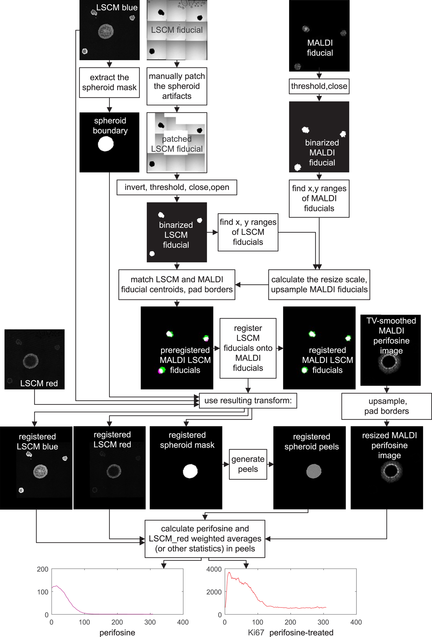
Fig. 6. Flowchart of MALDI MSI/LSCM multimodal spheroid peeling analysis. “LSCM blue” is the TO-PRO marker of cell nuclei, “LSCM red” is fluorescence of Ki-67 labeling proliferating cells, and the other signals belong to fiducial markers and the anti-cancer drug perifosine, as explained in the text. Spurious fiducial signals in the fluorescence images are ignored by the algorithm.
For colocalization, a transformation, which aligns the MALDI MS and LSCM images, has to be found. The transformation involves upsampling of the MALDI MS image to match the pixel size of the LSCM image, padding both the upsampled MALDI MSI and the LSCM signal to make their dimensions equal and applying an affine transformation to the LSCM images to bring the LSCM fiducials in register with their MALDI MSI counterparts.
The fiducial markers in binary form, which are eventually used for coregistration, are intermingled with other signals in both their MALDI MS and LSCM images.
In MALDI MSI, the fiducial markers yielded the strongest signal and at the same time good spheroid suppression in the m/z range of 597.2–597.6. To remove the remnants of the spheroid signal, the MALDI MS fiducial image was binarized by thresholding at 10% of its grayscale maximum. Any remaining isolated white spots were finally erased by a mathematical operation called morphological closing with a disk-shaped structuring element having a radius of 15 pixels (MATLAB functions imclose and strel).
The LSCM image of the fiducials was acquired in the transmission bright-field scan mode. In a mosaic created by software stitching the fiducials appear as black dots on bright background. The mosaic is distorted by a number of artifacts. Some mosaic borders are black as a result of the slight rotation of the respective tile. Also, there are visible air blobs with a dark boundary in some tiles. As these artifacts are irregular, we chose to replace them manually with white patches. The patched grayscale LSCM fiducial image is subsequently inverted, which turns the LSCM fiducials white, thresholded to make it binary, and despeckled by applying first morphological image closing and then opening with the disk-shaped structuring element of a 15 pixel radius again (MATLAB functions imclose, imopen, and strel).
Now that the binary images of white fiducials on a black background have been generated, the MALDI MS image needs to be upsampled. The resize scale is roughly estimated by measuring the distances of the outermost pixels of the fiducial markers in both binarized images in the horizontal and vertical direction, and the MALDI MS image is upsampled by a factor calculated as the ratio of the outer pixel distances in the LSCM and MALDI MS images. This makes the LSCM and the MALDI MS spatial resolution roughly identical, yet the images are still significantly shifted relative to each other. We prealign them with the aid of the three fiducial markers whose centroid coordinates are easily calculated. The two images are then shifted to make the centroids match. The prealignment is completed by padding the two fiducial images to obtain the same height and width, but they are still slightly rotated, and there may also be a minor scale difference. Therefore, the last transformation step consists of applying the MATLAB imregtform function, which finally yields the two registered MALDI MS and LSCM images of the fiducial markers. imregtform is also applied to the mask of the outer spheroid boundary.
At the end of image processing of drug-treated spheroids, peels are generated starting at the boundary of the coregistered LSCM spheroid mask. If colocalization of some particular m/z value such as the perifosine with another antibody distribution is required, the upsampling/padding steps are repeated for the MALDI MS image, and the transform resulting from coregistration is applied to the LSCM image of interest. Having done this, one can analyze the distance-dependent profiles of mean values, SDs, and other statistical values over the peels.
Peeling Analysis of Control Spheroids
To separate the effect of drug treatment on the distribution of proliferating, apoptotic, or necrotic cells from the influence of other factors, such as the supply of nutrients or oxygen, the perifosine-treated spheroids have to be compared with controls in which only cell staining was applied. The control slices are always prepared from a spheroid different from the drug-treated one. For the comparison to be conclusive, except for the missing drug treatment, the spheroids should be prepared equally in terms of staining, they should be equally old, and they should be imaged by LSCM in a quick sequence at the same microscope setting. These are only obvious prerequisites, and more research is needed to make images resulting from this kind of fluorescence imaging comparable, i.e., to quantify the LSCM images in some way.
Peeling analysis of the control spheroids does not include any MALDI MSI data, i.e., no coregistration of their LSCM images is necessary. With this exception, the procedure to establish cell distribution profiles in the peels is identical to that of the perifosine-treated spheroids: mask creation, generation of the peels, and computation of statistical data depending on the peel coordinate.
MATLAB Code for the Image Processing Pipeline
The above step-by-step description of the image processing pipeline is accompanied by our complete MATLAB code available at https://github.com/tandzin/Quantitative-MALDI-LSCM.
Results
In this section, we suggest how distance-dependent mean value profiles resulting from the peeling analysis of the mass spectrometry data and the fluorescence data can be used to detect dependence or causality between drug penetration and changes in cell abundance in the spheroid.
We restrict the presentation in the Results section to the case of LSCM images where both the perifosine-treated spheroid slice and the untreated control slice have been stained with two fluorescent markers:
• the TO-PRO marker which binds to cell nuclei and
• the Ki-67 marker which is associated with cell proliferation
Mean Value Profiles Resulting From Peeling Analysis of MALDI and IHC-Stained LSCM Images
Figure 7 shows an overlay of the high-resolution LSCM image of the Ki-67-stained spheroid coregistered with its low-resolution MALDI MS perifosine image.
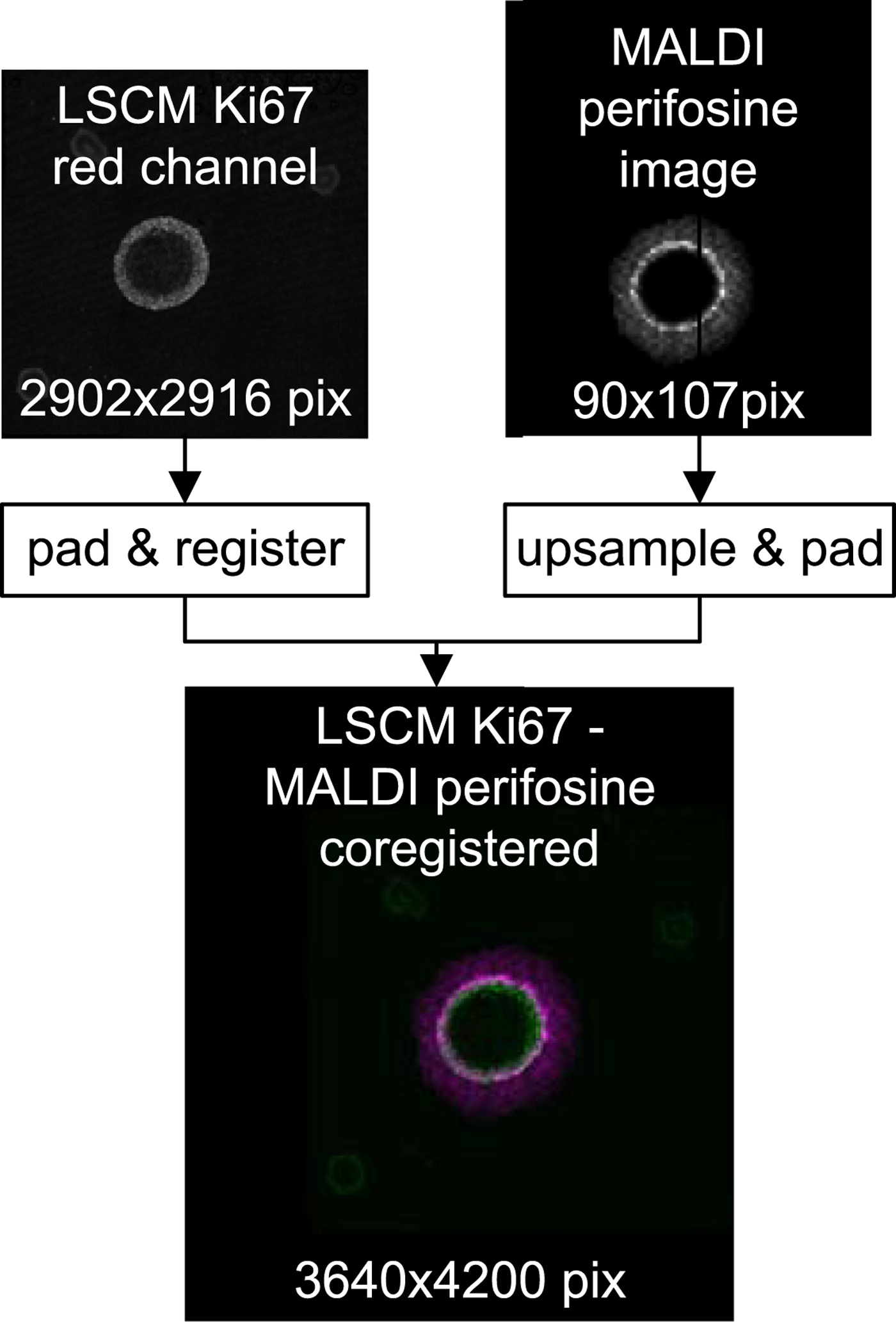
Fig. 7. Top row: raw LSCM and MALDI data before coregistration. Bottom: a false color overlay of coregistered LSCM and upsampled MALDI MSI data which serves as input for subsequent peeling analysis.
The upper two rows of Figure 8 shows on the left the coregistered LSCM and MALDI image of the perifosine-treated spheroid. The associated peel-dependent mean values of Ki-67-stained proliferating cells and the perifosine concentration are on the right.
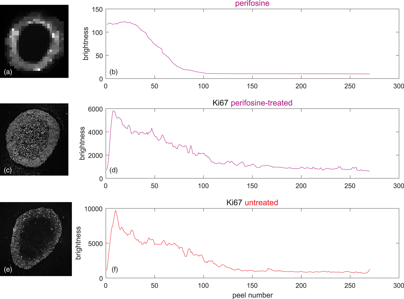
Fig. 8. Peeling analysis of a perifosine-treated and control (untreated) spheroid in equidistant peels, peel thickness = 1 pixel ~ 1.5 µm, averages weighted according to equation (5) by the signal of the TO-PRO marker of cell nuclei. (a) TV-smoothed MALDI MS image of perifosine, m/z range 462.4 ± 0.2, (b) corresponding average perifosine level in the peels, (c) LSCM image of the Ki-67 marker of proliferating cells, (d) average Ki-67 level corresponding to proliferating cells in the peels of the perifosine-treated spheroid, (e) LSCM image of untreated Ki-67-stained control spheroid, and (f) average Ki-67 levels corresponding to proliferating cells in the peels of the untreated spheroid.
Figures 8e and 8f show the LSCM image of a drug-untreated control spheroid and the associated mean values in the peels. It is seen that the level of the proliferating cells is higher than in the perifosine-treated spheroid.
Inferring Causation From Multimodal MALDI MSI and LSCM Fluorescence Data
Figures 8b and 8d show that the perifosine level and the numbers of proliferating cells are strongly correlated—both eventually decrease from the spheroid boundary inwards. However, the correlation does not necessarily imply that the number of proliferating cells is related to perifosine levels, because, in the Ki-67 profile of the untreated control spheroid (Fig. 8f) shortly after the boundary, the number of proliferating cells starts decreasing, too.
To verify if the perifosine treatment has caused any changes in proliferating cells, we propose to calculate the correlation of the perifosine profile with the difference between the treated and the control Ki-67 levels, as shown in Figure 9. If, apart from the drug treatment, the spheroid preparation, staining and the microscope setting were identical for the treated spheroid and the control, one can conclude that the change in cell abundance was caused by the application of the anti-cancer drug alone.
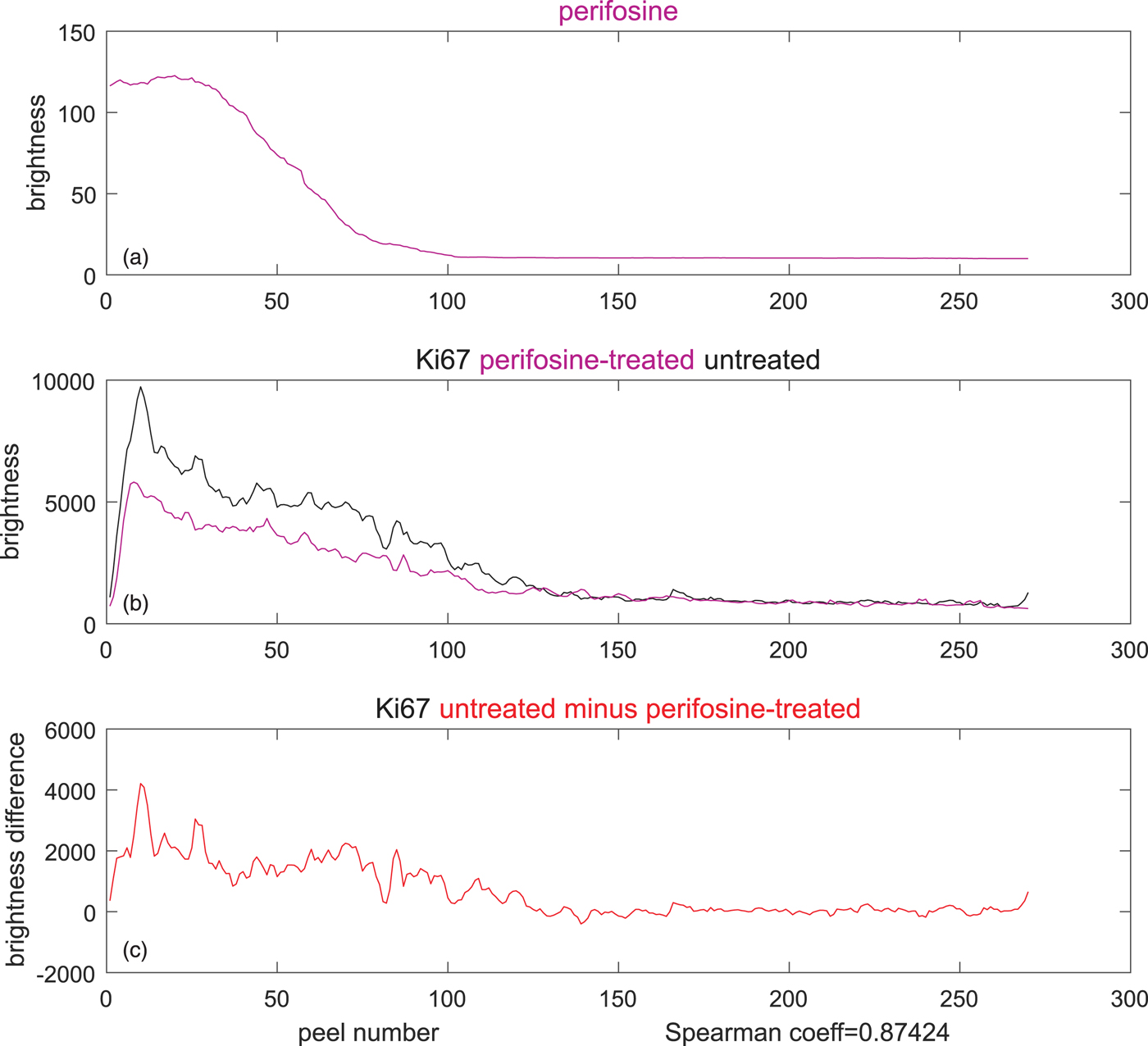
Fig. 9. Inferring causality from the difference of TO-PRO-weighted, Ki67-stained averages in the perifosine-treated (magenta), and control (untreated, black) spheroid. (a) Average perifosine values across the peels, (b) magenta: average Ki-67 in the peels of the perifosine-treated spheroid, black: average Ki-67 in the peels of the untreated spheroid, and (c) reduction of Ki-67 averages between the untreated and treated spheroids. The Spearman's correlation coefficient of 0.87 is very high.
To compute the correlation, we prefer the Spearman's correlation coefficient to the widely used Pearson's coefficient. The reason is that the Pearson's coefficient captures only linear dependencies between two variables, while the Spearman's coefficient evaluates correlation correctly also for monotonic nonlinear dependencies, as we explain in Supplementary Material. Its high value of 0.87 (bottom of Fig. 9) may suggest that the decrease in proliferating cells between the control and the drug-treated cells was caused by the perifosine treatment. However, this is yet to be confirmed by other methods.
Discussion
The present study demonstrates how two imaging modalities, mass spectrometry imaging and laser scanning fluorescence microscopy, can be combined to quantitatively assess the efficacy of new anti-cancer drugs using 3D models of cancerous tissue, the MCTS. Our contribution deals solely with image processing aspects of the project and does not attempt to draw any biological conclusions. These will be elaborated in a planned paper discussing the treatment of multicellular tumor models with anti-cancer drugs from the biological point of view. While the example in the Results section indicates that application of perifosine might reduce the number of proliferating cells, we do not claim that it really does—such a statement would have to be confirmed by additional methods.
The MALDI MS imaging is a semi-quantitative imaging modality where, in theory, the values returned by the mass spectrometer should be convertible to some physical quantity such as the concentration of some particular analyte at a specimen spot being illuminated by the laser. Our experience, however, suggests that factors such as the matrix thickness, fluctuation in the laser power and others affect the reproducibility of the mass measurement. While this makes pixel-by-pixel comparability of two MALDI MS images questionable, the comparison does make sense in our “peeling” approach where average values in the peels rather than individual pixels are compared. Furthermore, the proposed TV-based smoothing of the MALDI MS signal [equation (3)] makes MALDI MS measurements more plausible.
The fluorescence microscopy techniques we used are only qualitative in the sense that the image brightness cannot be readily converted to the abundance of the marker-specific cell type (proliferating, quiescent, apoptotic, or necrotic). If the specimens originate from equally old spheroids grown from the same cancer cell line and have been prepared by adopting exactly the same protocol, then, while still not quantifiable, the LSCM image brightness may at least qualitatively be related to the abundance of the respective cell type and allow comparison of the type “the specimen X has more of …/less of…”.
Under the assumption of comparability of MALDI MSI and LSCM measurements in the above sense, the method of discovering changes in Ki-67-marked cell amounts caused by anti-cancer drug points the way to obtaining quantitative data (such as the Spearman's coefficient) from the purely qualitative LSCM signals and the semi-quantitative MALDI MSI signal.
The example presented in the Results section uses the Ki-67 IHC marker of proliferating cells. For other stains (e.g., the cleaved caspase, the SNAIL/SLUG, or the lysyl oxidase) which bind to cells in another state, the reasoning concerning the increase/decrease in cell abundance as a result of drug treatment may have to be adjusted or reversed. Nevertheless, owing to the possibility to use different fluorescent stains targeted at specific proteins expressed during the cell cycle, our method of colocalization is more universal than other methods reviewed in the Introduction section.
While not elementary, the data processing pipeline presented in Figure 6 is straightforward. It has been tested on more than 60 MALDI MSI/LSCM datasets and has proved to be sufficiently robust. Only two (semi-) manual image processing steps are needed: generation of the spheroid boundary mask and patching of the original LSCM fiducial image. Rarely, the thresholds or the diameter of the structuring element employed to generate the MALDI MSI and LSCM fiducials may need to be tweaked. Except for that, no other user intervention is required, and the rest of the image processing outlined in Figure 6 completes fully automatically in 2 min on a plain Intel Core i5-6500 based desktop PC running at 3.2 GHz.
Future applicability of the presented multimodal MALDI MSI—LSCM data assessment will most importantly depend on improving comparability, or even better, achieving quantifiability of both MALDI MSI and LSCM measurements. Extensive research in this direction is needed.
As a non-negligible by-product of the image processing pipeline, we proposed and routinely used a simple, inexpensive, and efficient preparation of fiducial markers perfectly visible both in MALDI MSI and LSCM transmission bright-field scanning mode. We believe that this is a significant contribution to other research exploiting multimodal MALDI MS—optical imaging.
Supplementary material
To view supplementary material for this article, please visit https://doi.org/10.1017/S1431927619014983.
Acknowledgments
The present study was supported by the Grant Agency of Masaryk University (MUNI/G/0974/2016 and MUNI/A/1359/2019) and the Ministry of Education, Youth and Sports of the Czech Republic (MEYS CR) under the projects LTC17016, CEITEC 2020 (LQ1601), TRANS-MED (LQ1605). We further acknowledge the core facility CELLIM of CEITEC supported by the Czech-BioImaging large RI project (LM2015062 funded by MEYS CR) and ERDF (No. CZ.02.1.01/0.0/0.0/16_013/0001775) for their support with obtaining scientific data presented in this paper.


