


1. Introduction
The intriguing landscape of particles dispersed in turbulent flows has attracted tremendous attention over the past decades due to their extensive existence in nature and industry (Pedley & Kessler Reference Pedley and Kessler1992; Moffet & Prather Reference Moffet and Prather2009; Lundell, Söderberg & Alfredsson Reference Lundell, Söderberg and Alfredsson2011; Mittal, Ni & Seo Reference Mittal, Ni and Seo2020). The presence of particles could introduce an extra scale (the particle size) to the turbulent flows, which may alter the energy cascade of the turbulence and modulate the turbulent flow. For neutrally buoyant particles as considered in the present work, when the suspension is dilute and/or the particles are extremely small (Voth & Soldati Reference Voth and Soldati2017; Mathai, Lohse & Sun Reference Mathai, Lohse and Sun2020; Brandt & Coletti 2022), the particle-laden system could be simplified using the point-particle model by taking the dispersed particles as inertialess particles that could follow faithfully the surrounding flows. Typical situations applying the point-particle model include plankton in the ocean (Stocker Reference Stocker2012; Qiu et al. Reference Qiu, Mousavi, Zhao and Gustavsson2022) and pollen species in the atmosphere (Sabban & van Hout Reference Sabban and van Hout2011). For particles with higher volume fractions or non-negligible inertia, the interactions between particle and fluid can be modelled as two-way coupling using the point-particle method towards the motivation of investigating the particle dynamics and flow modulations (see the literature in the reviews Voth & Soldati Reference Voth and Soldati2017; Brandt & Coletti 2022). However, given its simplicity, the point-particle model could not account precisely for the feedback of particles on the surrounding flows in general situations, such as the particle boundary layer and the wake behind it (Jiang et al. Reference Jiang, Wang, Liu, Sun and Calzavarini2022). To this end, the finite-size particles, typically with diameters larger than the dissipation length scale  $\eta$ of the surrounding turbulent flows (Voth & Soldati Reference Voth and Soldati2017; Mathai et al. Reference Mathai, Lohse and Sun2020; Brandt & Coletti 2022), have been a vigorous field in recent years, in both experiments (Qureshi et al. Reference Qureshi, Bourgoin, Baudet, Cartellier and Gagne2007, Reference Qureshi, Arrieta, Baudet, Cartellier, Gagne and Bourgoin2008; Fiabane et al. Reference Fiabane, Zimmermann, Volk, Pinton and Bourgoin2012; Will et al. Reference Will, Mathai, Huisman, Lohse, Sun and Krug2021; Will & Krug Reference Will and Krug2021a,Reference Will and Krugb; Obligado & Bourgoin Reference Obligado and Bourgoin2022) and numerical simulations (Calzavarini et al. Reference Calzavarini, Volk, Bourgoin, Lévêque, Pinton and Toschi2009; Picano, Breugem & Brandt Reference Picano, Breugem and Brandt2015; Peng, Ayala & Wang Reference Peng, Ayala and Wang2020; Yousefi, Ardekani & Brandt Reference Yousefi, Ardekani and Brandt2020; Assen et al. Reference Assen, Ng, Will, Stevens, Lohse and Verzicco2022; Demou et al. Reference Demou, Ardekani, Mirbod and Brandt2022; Li, Xia & Wang Reference Li, Xia and Wang2022). In particular, by numerically implementing no-slip boundary conditions on their surface, the finite-size particles are capable of modelling the particle dynamics (Jiang, Calzavarini & Sun Reference Jiang, Calzavarini and Sun2020; Jiang et al. Reference Jiang, Wang, Liu, Sun and Calzavarini2022) and the resulting turbulence modulation (Ardekani et al. Reference Ardekani, Costa, Breugem, Picano and Brandt2017; Wang, Sierakowski & Prosperetti Reference Wang, Sierakowski and Prosperetti2017b; Ardekani & Brandt Reference Ardekani and Brandt2019).
One of the subjects of particle-laden turbulence in the non-dilute regime is the turbulence modulation caused by particles. Due to the no-slip boundary conditions at their surface, the finite-size particles could modulate the surrounding flow and the entire field, such as through shedding vortices in the wake region (Risso Reference Risso2018; Mathai et al. Reference Mathai, Lohse and Sun2020) and enhancing the dissipation rate around them (Jiang et al. Reference Jiang, Wang, Liu, Sun and Calzavarini2022). For particle-laden turbulence with neutrally buoyant particles, the system can be characterized by four dimensionless numbers, namely, the flow Reynolds number  $Re$, the size ratio of particle diameter to turbulence dissipation length scale $d_v/\eta$, the aspect ratio of particles $\lambda$, and the volume fraction of particles $\phi$. Among others, the aspect ratio of particles has been found to affect the clustering effects and particle dynamics, thus altering the magnitude of turbulence modulation. For instance, Ardekani & Brandt (Reference Ardekani and Brandt2019) found that the spherical particles could result in an overall drag enhancement, while the non-spherical particles might result in drag enhancement or reduction, depending on their aspect ratios. Similar findings on the turbulence modulation caused by non-spherical particles are also reported in their previous work (Ardekani et al. Reference Ardekani, Costa, Breugem, Picano and Brandt2017). In the view of turbulence, the aspect ratios of particles are found to affect their effects on the turbulence fluctuation intensity, thus altering the stress contributions (Ardekani & Brandt Reference Ardekani and Brandt2019).
In our previous experimental work in turbulent Taylor–Couette (TC) flow (Wang et al. Reference Wang, Yi, Jiang and Sun2022), it has been observed that the suspended spherical particles could result in a larger drag increase than for the non-spherical particles. By proposing a qualitative analysis of the stress balance, the drag increases caused by the suspended particles are explained. On the other hand, it is observed that the clustering effects of particles are affected by the aspect ratio of particles. The spherical particles show clustering near the walls, whereas the non-spherical particles cluster preferentially in the bulk region. Based on the previous numerical studies of finite-size particles (Ardekani et al. Reference Ardekani, Costa, Breugem, Picano and Brandt2017; Ardekani & Brandt Reference Ardekani and Brandt2019), it is conjectured that the preferential clustering of particles could be responsible for their different magnitudes of turbulence modulation. However, limited by the experimental techniques, an in-depth and more quantitative analysis is absent on several aspects, specifically the following. (i) How and to what extent is the basic turbulent flow modulated by the suspended particles with different aspect ratios? (ii) How are the particle statistics affected by their aspect ratios? (iii) What is the difference in the turbulence modulation between the near-wall clustering of spherical particles and the bulk clustering of non-spherical particles?
We should note that although similar phenomena have been reported for channel flows, the difference of shear flow from the channel flow could give rise to new physics and observations. For example, the findings on drag modulation in Wang et al. (Reference Wang, Yi, Jiang and Sun2022) indicate that, regardless of the particle aspect ratio, only drag increments are possible for particle-laden TC flow. However, numerical studies in channel flows have found drag reduction in the cases of oblate particles (e.g. Ardekani & Brandt Reference Ardekani and Brandt2019), leaving open the question of whether this is a physical feature of channel flow or simply a numerical artefact. To resolve this issue, we can perform simulations in shear flows similar to those used in experiments on TC flow. In fact, unlike the pressure-driven channel flow, which has a parabolic velocity profile and yields the maximum velocity and zero velocity gradient at the channel centre, the Couette flow shows a non-zero gradient at the domain centre. The difference in velocity profile could affect the velocity fluctuation and thereby the stress balance (drag) in the fluid phase. Additionally, the particle statistics are affected by the velocity profile of the flow as their dynamics is related to the velocity gradient tensor of the flow (Voth & Soldati Reference Voth and Soldati2017). Therefore, investigating the shear flows laden with particles is of great interest.
To this end, this work aims to conduct fully particle-resolved direct numerical simulations (PR-DNS) to provide a quantitative analysis of our previous experimental results and answer the aforementioned questions. Performing simulations in TC flow is computationally expensive because it requires not only processing cylindrical geometries but non-uniform grid spacing to resolve the boundary layers in the radial direction. Hence we employ a configuration of plane-Couette flow to carry out our investigation, which is of Cartesian coordinates and can be implemented efficiently with a scheme based on the lattice Boltzmann method. Using the immersed boundary method (Peskin Reference Peskin2002), we can resolve the motion of each particle and its surrounding flow field, allowing us to uncover the physics of both particle dynamics and the resulting turbulence modulation. The rest of the paper is organized as follows. Section 2 describes the flow configuration and numerical schemes. In § 3, we discuss the results, including the turbulent arguments and the particle statistics. Section 4 gives final remarks on this work.
2. Numerical methodology
2.1. Configurations of flow and particles
We conduct simulations with spheroidal particles suspended in a turbulent plane-Couette flow. The flow configurations are depicted in figure 1. Two walls are moving in opposite directions with constant velocity  $U$. No-slip boundary conditions are imposed on the walls, while the flow in the streamwise and spanwise directions is periodic. The turbulent flow is governed by the conservation equations of momentum and mass, which read as
 $$\begin{gather} \partial_t \boldsymbol{u} + \boldsymbol{u}\boldsymbol{\cdot}\boldsymbol{\nabla}\boldsymbol{u} ={-}\rho^{{-}1}\,\boldsymbol{\nabla} p +\nu\, \nabla^2\boldsymbol{u}+\boldsymbol{f}_p, \end{gather}$$
 $$\begin{gather}\boldsymbol{\nabla} \boldsymbol{\cdot} \boldsymbol{u} = 0, \end{gather}$$
where  $\boldsymbol {u}$ and $p$ are the velocity vector and hydrodynamic pressure field of the flow, and $\rho$ and $\nu$ are the density and viscosity of the fluid. Since the suspensions are composed of finite-size particles and in the non-dilute regime, the particle can modulate the surrounding turbulence by exerting feedback force $\boldsymbol {f}_p$ on the flow. The turbulence intensity can be quantified by the bulk Reynolds number (hereafter, the Reynolds number)
 \begin{equation} Re = Uh/\nu, \end{equation}
where  $\nu$ is the kinematic viscosity of the fluid, and $h$ is the half-width of the domain in the wall-normal direction. Alternatively, the turbulence intensity can also be related to the shear Reynolds number,
 \begin{equation} Re_\tau = u_\tau h/\nu, \end{equation}
where  $u_\tau = \sqrt {\tau _w/\rho }$ is the friction velocity, with $\tau _w$ being the shear stress at walls. The values of $Re$ and the corresponding $Re_\tau$ are presented in table 1. In this work, the values of $Re$ are set based on those in our previous experimental work. We note that in TC flow (Wang et al. Reference Wang, Yi, Jiang and Sun2022), the Reynolds number is defined as $Re_e = (u_i-u_o)d/\nu$, where $u_i$ ( $u_o$) is the velocity of the inner (outer) wall, and $d$ is the gap width between walls. Hence the values of $Re$ in the present work are one-quarter of the corresponding values of $Re_e$ reported in Wang et al. (Reference Wang, Yi, Jiang and Sun2022) (see table 1).

Figure 1. Sketch of the flow configuration. Two walls are moving at constant velocities in opposite directions. For particle-laden cases, particles with three kinds of aspect ratios are randomly suspended at the beginning and then move freely in the domain box.
Table 1. Simulation parameters:  $Re$ is the bulk Reynolds number defined by the wall velocity $U$ and half-width of the gap $h$, which is therefore one-quarter of the corresponding values of $Re_e$ reported in Wang et al. (Reference Wang, Yi, Jiang and Sun2022), defined by the difference of wall velocity $(u_i-u_o) = 2U$, and the gap width $d=2h$. Here, $Nx \times Ny \times Nz$ is the number of grids in each direction, $d_v/Ly$ and $d_v/\eta$ are the ratios of the equivalent-volume diameter of particles to the width of the domain in the wall-normal direction and to the dissipation length scale, respectively, $\lambda$ and $\phi$ are the aspect ratio and the volume fraction of particles, $Re_\tau$ is the friction Reynolds number defined by (2.4), $Re^{slip}_p$ is the particle Reynolds number based on the global mean slip velocity, $Re_p^{\lambda }=Ud_v^2/h\nu ^2$ is the particle Reynolds number based on local shear, $\varDelta /\delta _\nu$ and $\varDelta /\eta$ are the grid spacing normalized by the viscous length scale $\delta _\nu$ and the dissipation length scale $\eta$, $u_\tau T/h$ indicates the running times in terms of turnover periods for eddies of size $h$ and velocity $u_\tau$, $\delta _{\tau _w}/\bar {\tau }_w$ gives the statistic errors for each case, where $\delta _{\tau _w} = \tau _w|_{y=2h}-\tau _w|_{y=o}$ is the difference of wall stress, and $\bar {\tau }_w = (\tau _w|_{y=2h}+\tau _w|_{y=o})/2$ is the mean wall stress.

Neutrally buoyant spheroids are studied with different parameters, including the equivalent-volume diameter  $d_v$, the aspect ratio $\lambda$, and the volume fraction $\phi$, chosen based on our previous experimental work (Wang et al. Reference Wang, Yi, Jiang and Sun2022). Here, for a spheroidal particle, we have $d_v = (h_pd_p^2)^{1/3}$ and $\lambda = h_p/d_p$, where $d_p$ is the length of the symmetric axis of the particle, and $h_p$ is the length perpendicular to it (see figure 1). The parameters of particles are given in table 1. The particle motion is governed by the Newton–Euler equations as
 $$\begin{gather} m_p\,\frac{\mathrm{d} \boldsymbol{v}}{\mathrm{d}t} = \boldsymbol{F}+ \boldsymbol{F}_c, \end{gather}$$
 $$\begin{gather}\frac{\mathrm{d} \boldsymbol{I}_p\boldsymbol{\varOmega}}{\mathrm{d}t} = \boldsymbol{T}+ \boldsymbol{T}_c, \end{gather}$$
where  $\boldsymbol {v}(t) = \mathrm {d} \boldsymbol {r}/ \mathrm {d} t$ and $\boldsymbol {\varOmega }(t)$ are the particle velocity and angular velocity vectors of a particle at position $\boldsymbol {r}(t)$ with mass $m_p = \rho _p V_p$ (with $\rho _p$ the particle density and $V_p$ the volume), and $\boldsymbol {I}_p$ is the moment of inertia tensor. In the right-hand sides of the above equations, $\boldsymbol {F}$ is the force exerted on particles by the surrounding fluid through hydrodynamics, while $\boldsymbol {F}_c$ is the collision force accounting for the particle–particle and particle–wall collisions; $\boldsymbol {T}$ and $\boldsymbol {T}_c$ are the torques defined in similar ways.
At  $Re=1600$, two values of $\phi$ are chosen to study its effects on turbulence modulation, whereas at $Re=3200$, only the case of small $\phi$ ( $\phi = 2\,\%$) is conducted due to the costly computational expense at the high volume fraction case, which nonetheless could uncover the roles of turbulent intensity. For each $Re$ case, we first run the cases of single-phase flow (i.e. $\phi =0\,\%$) to generate a fully developed plane-Couette turbulence. Then the particle-laden case is conducted by randomly dispersing the particle in the entire domain with an initial velocity equal to zero. Statistical equilibrium is ensured by reaching time-averaged statistical errors in wall stress typically less than $1\,\%$ (see table 1).
2.2. Numerical schemes
In this subsection, we describe briefly the numerical schemes used to simulate the particle suspension. The turbulence is solved numerically using an open-source code with the lattice Boltzmann method, the ch4-project (Calzavarini Reference Calzavarini2019), which has been validated extensively in particle-laden turbulence both for point-like particles (Mathai et al. Reference Mathai, Calzavarini, Brons, Sun and Lohse2016; Calzavarini, Jiang & Sun Reference Calzavarini, Jiang and Sun2020; Jiang et al. Reference Jiang, Wang, Liu, Sun and Calzavarini2021) and finite-size particles (Jiang et al. Reference Jiang, Calzavarini and Sun2020, Reference Jiang, Wang, Liu, Sun and Calzavarini2022). The code was validated by comparing the translational dynamics of spheres at  $Re_\lambda = 32$ with a previous reference study (Homann & Bec Reference Homann and Bec2010). The details and validations of the code can be found in our previous work (Jiang et al. Reference Jiang, Wang, Liu, Sun and Calzavarini2022).
On the fluid-phase side, the domain size is  $Lx \times Ly \times Lz = 4h \times 2h \times 2h$, where $Lx, Ly, Lz$ are the widths of the domain in the streamwise, wall-normal and spanwise directions, respectively. Here, we note that the domain size is chosen based on producing fully developed turbulence, which for the current $Re$ ranges is $Lx/Ly \simeq 2$ (Owolabi & Lin Reference Owolabi and Lin2018). To double check if the domain size is long enough and the artefacts of periodic boundary conditions affect the results, we run an additional case with $Lx \times Ly \times Lz = 8h \times 2h \times 2h$. It is found that the drag coefficient (see the blue square in figure 2a) and the particle statistics (figure 11b) are comparable to the cases reported in table 1. Therefore, the domain size in table 1 is long enough to yield conclusive results. The computational domain is meshed by grids distributed uniformly in each direction, and the numbers of grids, $Nx \times Ny \times Nz$, is given in table 1. Considering the requirement of the numerical resolution, the maximum grid spacing is validated to be $\varDelta \leq 1.1\delta _\nu$ and $\varDelta \leq 0.68\eta$ at $Re = 1600$ (see table 1), where $\delta _\nu = \nu /u_\tau$ is the viscous length scale, and $\eta = (\nu ^3/\epsilon )^{1/4}$ is the dissipation length scale, with $\epsilon$ the global dissipation rate of the flow. In consequence, about five grids are embedded in the linear viscous layer (as can be seen in figure 5). Hence the grid spacing adopted in all runs is sufficient to resolve the turbulence fluctuation and flow structures, in both the boundary layers and the bulk.

Figure 2. Normalized wall stress for particle-laden cases. The experimental data (empty circles) are adapted from the TC experiments (Wang et al. Reference Wang, Yi, Jiang and Sun2022). The blue square in (a) denotes the result of the validation case of extended domain size in the streamwise direction ( $Lx \times Ly \times Lz = 8h \times 2h \times 2h$). The values of $Re$ and $\phi$ are shown in each plot.
On the particle-phase side, the particle–fluid interaction is fully resolved by employing the immersed boundary method (IBM; Peskin Reference Peskin2002). The IBM enforces the no-penetration and no-slip boundary conditions at the fluid–particle interface by means of a localized feedback force  $\boldsymbol {f}_p$, added to (2.1). Such an $\boldsymbol {f}_p$ term is also denoted as two-way coupling. The particle surfaces are captured by uniformly distributed Lagrangian nodes. Adequate grids are required to resolve the flow around particles. The test towards this has been carried out in our previous work (Jiang et al. Reference Jiang, Wang, Liu, Sun and Calzavarini2022). It is found that at least 16 grids per particle diameter are needed to resolve the particle boundary layers. In this work, we surpass this criterion to attain convincing results. Specifically, for the cases $Re=1600$ and $3200$, we use 19 and 26 grids per particle diameter, respectively, to resolve the particle boundary layers and their dynamics. To ensure high accuracy for the implementation of the no-slip fluid boundary condition at the particle surface, we adopt the so-called IBM multi-forcing scheme with 5-step iterations; see Luo et al. (Reference Luo, Wang, Fan and Cen2007) and Wang et al. (Reference Wang, Jiang, Jiang, Sun and Liu2021). The processes of particle–particle and particle–wall collisions are implemented by means of soft-sphere collision forces (Costa et al. Reference Costa, Boersma, Westerweel and Breugem2015; Ardekani et al. Reference Ardekani, Costa, Breugem and Brandt2016) and lubrication corrections (Brenner Reference Brenner1961; Cooley & O'Neill Reference Cooley and O'Neill1969; Costa et al. Reference Costa, Boersma, Westerweel and Breugem2015; Ardekani et al. Reference Ardekani, Costa, Breugem and Brandt2016), where $\boldsymbol {F}_c$ and $\boldsymbol {T}_c$ can be computed. The details of the calculations of the hydrodynamic force and torque can be found in our previous work (Jiang et al. Reference Jiang, Wang, Liu, Sun and Calzavarini2022). In our simulations with the IBM, the boundary of the finite-size particle is represented by Lagrangian nodes, and the particle–fluid interactions are solved by the delta function as suggested by Peskin (Reference Peskin2002). Furthermore, we seed Lagrangian points inside the finite-size particle that are fixed in the particle frame. These Lagrangian points are used to measure the momentum time derivative of fluid inside the finite-size particle to obtain the correct driving force. And we use the trilinear scheme to interpolate the velocities of the Lagrangian points inside the finite-size particle. The Newton–Euler equations that govern the particle dynamics are integrated numerically with a second-order Adams–Bashforth time-stepping scheme.
Since the size ratio  $d_p/\eta$ is fixed, the numbers of particles $Np$ are determined by their volume fractions, yielding $Np=76$ and $229$ for the cases $\phi =2\,\%$ and $6\,\%$, respectively. Therefore, the statistical convergence of the numerical wall stress and the particle statistics is ensured by running the simulation long enough to get sufficient data. The running time for each case is given in table 1. For additional information, the time series of the fluid and particle velocity fluctuations are shown in the Appendix.
3. Results and discussion
3.1. Turbulence modulation: global drag, velocity field and dissipation rate
We start by comparing the global turbulence modulation of numerical results to that of experimental measurements (Wang et al. Reference Wang, Yi, Jiang and Sun2022). The global transport quantity of plane-Couette turbulence is the shear stress at the walls,
 \begin{equation} \tau_{w,\phi} = \rho\nu \left.\frac{\mathrm{d}U_f}{\mathrm{d} y}\right|_{y=0,2h}, \end{equation}
where  ${\mathrm {d}U_f}/{\mathrm {d} y}|_{y=0,2h}$ is the gradient of mean streamwise velocity at the walls. We normalize the wall stress of particle-laden flow by that of single-phase flow, i.e. $\tau _{w,\phi }/\tau _{w,\phi =0}$, and show it in figure 2, where the results from previous experiments in TC flow (Wang et al. Reference Wang, Yi, Jiang and Sun2022) are also depicted for comparison. As we keep the flow parameters the same, the discrepancies between numerics and experiments could be attributed to the different flow configurations. Although both flow configurations are shear-induced flows, TC flow suffers from more complex conditions, such as the cylindrical geometries causing asymmetric velocity profiles in the radial direction, and the strong confinement due to the end-plates which cause secondary flow (Grossmann, Lohse & Sun Reference Grossmann, Lohse and Sun2016). It is therefore not expected to observe exact agreement between the numerical results and experiments. Moreover, as the particle dynamics is affected by aspect ratios (Voth & Soldati Reference Voth and Soldati2017), the spherical and non-spherical particles could respond in different ways as the flow configuration changes, therefore resulting in different responses in drag modulation. This could possibly account for the fact that in drag modulation (figure 2), compared to non-spherical particles, the spherical particles show better agreements in TC flow and plane-Couette simulations. Nevertheless, since we are interested mainly in the effects of particle aspect ratio on the turbulence modulation, the conclusion can be drawn that the spherical particles could cause larger drag modulations than the non-spherical particles, for different $Re$ and $\phi$ with the numerical results in figure 2. Similar findings are also reported in our previous experimental TC flows, where the difference in magnitude of drag modulation between spherical and non-spherical cases is not obvious at the present $\phi$ ( $\varDelta _{c_f/c_{f,\phi =0}}\sim 1\,\%$; see figure 2) but becomes larger at a higher value of $\phi$ ( $\varDelta _{c_f/c_{f,\phi =0}}\sim 5\,\%$ at $\phi =10\,\%$).
For fixed  $Re$ and $\lambda$ (see figures 2a,b), the magnitudes of drag modulation increase with increasing $\phi$, which again agrees with the results in our previous experimental measurements (Wang et al. Reference Wang, Yi, Jiang and Sun2022). To demonstrate this $\phi$ dependence of drag modulation, in figure 3 we present the velocity fields and corresponding fields of dissipation rate at the centre plane in the streamwise direction (i.e. $x=Lx/2$). For clarity, only the case of the spherical particles at $Re=1600$ is shown. Compared to the single-phase case (figure 3a), the presence of particles could introduce strong disturbance in both the bulk and boundary layers; see the emergence of the higher value of dissipation rate coloured in red around the particles in figures 3(b,c). On the other hand, figure 4 shows information similar to that in figure 3 but for different $\lambda$ at $Re=1600$ and
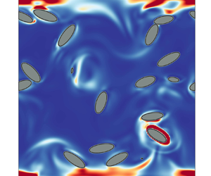
  $\phi =6\,\%$. It can be seen that the particle could modify the surrounding fields and particularly enhance the dissipation rate near their surface, which again could be related to the particle boundary layers (Jiang et al. Reference Jiang, Wang, Liu, Sun and Calzavarini2022) and accounts for the drag increases reported in figure 2. This enhancement of turbulence dissipation of particles has been found in other flows, e.g. homogeneous and/or isotropic turbulence (Cisse, Homann & Bec Reference Cisse, Homann and Bec2013; de Motta et al. Reference de Motta, Estivalezes, Climent and Vincent2016; Jiang et al. Reference Jiang, Wang, Liu, Sun and Calzavarini2022) and decaying isotropic turbulence (Lucci, Ferrante & Elghobashi Reference Lucci, Ferrante and Elghobashi2010). Due to the no-slip condition enforced at the particle surface, a local force arises on the fluid surrounding the particle, which locally increases the velocity gradients close to the particle surface and thus increases the local strain rate as well as the dissipation rate (Lucci et al. Reference Lucci, Ferrante and Elghobashi2010). As the distance to the particle surface increases, this impact of the no-slip condition fades, and so does the dissipation rate. This accounts for the observations in figures 3 and 4, where the bursts of high dissipation rate (coloured in red) occur only near the particles, while the rear fluid remains almost undisturbed (coloured in blue). Indeed, the particles are found to enhance the dissipation rate around them to a distance of about one radius to their surfaces (Cisse et al. Reference Cisse, Homann and Bec2013; de Motta et al. Reference de Motta, Estivalezes, Climent and Vincent2016) for spherical particles, while for non-spherical particles, the volume of disturbed fluid is smaller in every dimension (Jiang et al. Reference Jiang, Wang, Liu, Sun and Calzavarini2022). Additionally, the enhancement of the dissipation rate around particles distributes in a non-uniform manner; namely, the dissipation rate in front of the particle is higher than in the rear of the particles (Cisse et al. Reference Cisse, Homann and Bec2013; de Motta et al. Reference de Motta, Estivalezes, Climent and Vincent2016). Although this cannot be quantified in the present work, it can still be hinted from figures 3(e, f) and 4(d–f), where the dissipation rate around particles is asymmetric. With increasing volume fraction of particles, the dissipation rate becomes pronounced, as could be seen in figures 3 and 4. This is due to the increase of particle surface area that affects the surrounding fluid and thus the two-way coupling force (Lucci et al. Reference Lucci, Ferrante and Elghobashi2010). Moreover, a closer look would find that the spherical particles cause stronger disturbances to the boundary layers, while the non-spherical particles alter mainly the flow in the bulk.

Figure 3. Instantaneous snapshots of (a–c) streamwise velocity indicated by the colour bar, where the overlaid arrow vectors depict flow velocity within the plane, and (d–f) dissipation rate. Data are obtained from the cases of spherical particles (SP,  $\lambda = 1$) at $Re=1600$, for (a,d) $\phi =0\,\%$, (b,e) $\phi =2\,\%$, and (c, f) $\phi =6\,\%$.

Figure 4. Instantaneous snapshots of (a–c) streamwise velocity indicated by the colour bar, where the overlaid arrow vectors depict flow velocity within the plane, and (d–f) dissipation rate. Data are obtained at  $Re=1600$ and $\phi =6\,\%$, for (a,d) $\lambda = 1/3$, (b,e) $\lambda = 1$, and (c, f) $\lambda = 3$.
We depict the profiles in the wall-normal direction of streamwise velocity and dissipation rate in figures 5 and 6, respectively. In figure 5, the velocity profile is shown in the wall units, where  $y^+ = y/\delta _\nu$ is the distance from the lower wall ( $y=0$) in units of the viscous length scale $\delta _\nu$, and $u^+ = (u-u|_{y=0})/u_\tau$ is the velocity difference from the lower wall normalized by the friction velocity $u_\tau$. For comparison, we also depict the viscous sublayer $u^+=y^+$ and the logarithmic law of flat turbulent boundary layer flow, i.e. $u^+= (1/\kappa )\ln y^++B$ with the typical values $\kappa =0.40$ and $B=5.2$ as suggested by Prandtl and von Kármán (Pope Reference Pope2000). One can see that, regardless of the values of $\phi$ and $\lambda$, the profile of $u^+=y^+$ is well retained with sufficient grids inside the viscous sublayer ( $y^+<5$), which is barely affected by the suspended particles due to their finite sizes (see the vertical dotted lines in figure 5). Outside the viscous sublayer, the velocity profiles generally follow the logarithmic law in all cases. The effects of particle aspect ratio become pronounced with increasing $\phi$ (see figure 5b). Compared to single-phase flow, the cases of particle-laden flow result in the velocity profile consisting of an extended logarithmic layer, which is similar to the observation in channel flow (Eshghinejadfard, Zhao & Thévenin Reference Eshghinejadfard, Zhao and Thévenin2018) and yields in the reduced velocity gradient in the near-wall region. This seems to contradict the drag increases reported in figure 2. However, as shown later, for particle-laden flow the dampening in velocity does not imply a global drag reduction since there are extra stress contributions from the particle phase. Moreover, in terms of the effect of particle aspect ratio, it is found that at fixed $Re$ and $\phi$, the spherical particles cause greater velocity reduction than the non-spherical particles in the logarithmic layer (e.g. see figure 5b). Specifically, in figure 5(b), the value of $B$ of spherical particles ( $B\simeq 2.3$) is smaller than that of non-spherical particles ( $B\simeq 3.5$), while the values of $\kappa$ are close to $0.40$ in all particle-laden cases. This is consistent with the drag increase found in figure 2 since the decrease in $B$ indicates a drag enhancement, and the decrease in $\kappa$ does the opposite (Ardekani et al. Reference Ardekani, Costa, Breugem, Picano and Brandt2017).

Figure 5. Velocity profiles depicted in the wall units. The vertical dotted and dashed lines indicate, respectively, the location of the equivalent-volume radius of particles ( $r_v=d_v/2$) and the location of the central plane in the wall-normal direction ( $y=h$).

Figure 6. Profiles of dissipation rate. The insets show the zoom-in view of the dissipation rate in the near-wall region. The error bars are shown to indicate the numerical uncertainty. For clarity, only the most noticeable error bars (next to the walls) in the case of spherical particles are shown.
As for the dissipation rate (figure 6), its magnitudes agree well with the magnitudes of drag increases found in cases of different particle aspect ratios. We note that though the non-spherical particles could alter the bulk flow more strongly than the spherical ones in the bulk region (see figure 4), the dissipation rates in the bulk are minor contributions to the total field, resulting in negligible changes of the profiles of dissipation rate in that region (figure 6). In contrast, spherical particles efficiently increase the dissipation rate more than non-spherical particles near the walls (see insets in figure 6). This is in line with the magnitudes of global drag modulation of particles with different  $\lambda$ because, as for the wall stress, the dissipation rate in the near-wall region is positively associated with the velocity gradient at the walls.
3.2. Turbulence modulation: stress analysis and turbulent energy spectra
In the previous work (Wang et al. Reference Wang, Yi, Jiang and Sun2022), we decompose the total stress (i.e. the shear stress at walls  $\tau _{w,\phi }$) into four terms, namely, the viscous stress of the fluid phase ( $\tau _\nu$), the turbulent stress of the fluid and particle phases ( $\tau _{Tf}$ and $\tau _{Tp}$, respectively), and the particle-induced stress ( $\tau _p$), which can be written as
 \begin{equation} \tau_{w,\phi} = \tau_\nu+\tau_{Tf}+\tau_{Tp} +\tau_{p}, \end{equation}
where  $\tau _{w,\phi }$ is defined by (3.1). For each term on the right-hand side, one can express it explicitly as suggested by Batchelor (Reference Batchelor1970), Zhang & Prosperetti (Reference Zhang and Prosperetti2010), Picano et al. (Reference Picano, Breugem and Brandt2015), Wang, Abbas & Climent (Reference Wang, Abbas and Climent2017a) and Wang et al. (Reference Wang, Yi, Jiang and Sun2022), in the form of turbulence quantities, as
 $$\begin{gather} \tau_{\nu} = \rho\nu (1-\phi)\,\frac{\mathrm{d} U_f}{\mathrm{d} y}, \end{gather}$$
 $$\begin{gather}\tau_{Tf} ={-}\rho(1-\phi)\,\langle u^{\prime}_fv^{\prime}_f \rangle, \end{gather}$$
 $$\begin{gather}\tau_{Tp} ={-}\rho \phi\,\langle u^{\prime}_pv^{\prime}_p \rangle, \end{gather}$$
 $$\begin{gather}\tau_{p} = \phi\,\langle \sigma^p_{xy} \rangle, \end{gather}$$
where  $u^{\prime }$ and $v^{\prime }$ are the velocity fluctuations in the streamwise and wall-normal directions, with the subscripts $f$ and $p$ denoting fluid and particle phase, respectively. Also, $\sigma ^p_{xy}$ is the general stress in the particle phase, projected in the streamwise plane and pointing in the streamwise direction, and $\langle \cdot \rangle$ means ensemble-averaged in time and over the streamwise plane. For the case of single-phase flow, the latter two terms are zero.
By means of numerics, we can look into the contributions of each term on the right-hand side of (3.2) to the total stress. The particle-induced stress  $\tau _p$ is calculated indirectly (i.e. $\tau _p = \tau _w-\tau _\nu -\tau _{Tf}-\tau _{Tp}$) as the explicit expression of $\sigma ^p_{xy}$ remains unknown currently. In figure 7, we plot the profile of stress balance in the wall-normal direction for each case, where we normalize each term of stress by the total stress of that case, i.e. $\tau /\tau _{w,\phi }$. We first demonstrate how the particle aspect ratio $\lambda$ affects the contributions of each stress at given $Re$ and $\phi$ (see each row of figure 7). Taking the case $Re=1600$ and $\phi =2\,\%$ as an example (figures 7a–c), one can see that the particle aspect ratio has slight effects on $\tau _\nu$ and $\tau _{Tf}$. Similarly, the turbulent stress of the particle phase, $\tau _{Tp}$, depends only weakly on $\lambda$ while having a positive dependence on $\phi$ (see figures 7d–f). However, the particle-induced stress, $\tau _p$, is affected by the particle aspect ratios to a noticeable extent, which becomes even more pronounced at high $\phi$ (see figures 7d–f). Since $\tau _p$ is the combined results of hydrodynamic interaction and particle collisions (Picano et al. Reference Picano, Breugem and Brandt2015), its value could be related to both the particle dynamics and the turbulence field. As the numerical errors from $\tau _p$ cannot be excluded now, we take the case of high $\phi$ (figures 7d–f), where the numerical errors are of less significance, as an instance to illustrate the effects of $\lambda$ on $\tau _p$. First, it is noticeable that for all $\lambda$ cases, $\tau _p$ reaches its peak near the walls. Near the walls, the spherical particles cause more pronounced peaks than the non-spherical particles in $\tau _p$, which validates our conjectures in previous work (Wang et al. Reference Wang, Yi, Jiang and Sun2022) and is in line with the findings in other configurations of particle-laden flow (Picano et al. Reference Picano, Breugem and Brandt2015; Ardekani et al. Reference Ardekani, Costa, Breugem, Picano and Brandt2017). As shown by the particle statistics in the later section, for spherical cases the occurrence of near-wall peaking in $\tau _p$ could originate from their near-wall preferential clustering, which could cause the particle collisions to happen in easier and more intense ways.


It is noticeable that for the oblate case ( $\lambda =1/3$, see figure 7d), $\tau _p$ becomes negative in the bulk region. As the results are ensured convergence by running the simulation long enough in time, the fact that it is negative could be attributed to the hydrodynamic interaction caused by the particles. This indicates that $\tau _p$ could be a stress sink under specific conditions. Similar overall drag reductions caused by particles have also been reported in simulation results in channel flow (Ardekani & Brandt Reference Ardekani and Brandt2019). However, we should note that the previous experimental results (Wang et al. Reference Wang, Yi, Jiang and Sun2022) report that only drag enhancement is observed in particle-laden flow under similar parameter regimes, even for the cases of oblate particles. This is in contrast to the current simulation results, where the particle-induced stress is found to be negative (figure 7d), and overall a drag (stress) reduction is observed (figure 8). In this sense, the particle-induced stress being negative in the bulk could be a numerical artefact, though there are differences in TC and plane-Couette flows as we mentioned before. Future study is needed to uncover the role of $\tau _p$. Moreover, the profiles in figure 7 are not exactly symmetric, especially in the particle-induced stress ( $\tau _p$). This could be due to the limitations of statistics as the particle numbers determined by its volume fraction are relatively small, which could cause inhomogeneity in the bounded wall-normal direction (i.e. the $y$-direction). Although extending the simulation time steps might improve the data quality, as we did for the spherical cases (see the values of $u_\tau T /h$ in table 1), the asymmetries are still present in the spherical cases. Nonetheless, the asymmetric amplitude is typically less than 5 % for all simulation cases, thereby the main conclusion on the stress analysis can be convincing. On the other hand, as $Re$ increases (see figures 7g–i), the profiles of stress coming from the particle phase ( $\tau _{Tp}$ and $\tau _p$) become almost flat. In these cases, the total stress is dominated by the viscous stress in the boundary layers and by the fluid-phase turbulence stress in the bulk, which is actually reminiscent of the case of single-phase flow.

Figure 8. Contributions of each individual stress to the total shearing stress. The total shearing stress of the corresponding single-phase cases (i.e.  $\tau _{w,\phi =0}$ at given $Re$) is used for normalization.
The contribution ratio of each stress to the total one can be found in figure 8, where we normalize each stress by the total shear stress at the walls of the single-phase cases, i.e.  $\tau /\tau _{w,\phi =0}$. For small $\phi$ (see figures 8a,c), it can be seen that the total stress is almost dominated by the viscous stress and the turbulent stress, while the presence of particles negligibly affects the stress of the flow. The changes in $Re$ mainly redistribute the contributions from $\tau _\nu$ and $\tau _{Tf}$ to the total stress. With increasing $\phi$ (see figure 8b), the role of particles becomes pronounced, as indicated by the greater contributions of $\tau _{Tp}$ and $\tau _p$. Indeed, one can see that the stress coming from the particle phase could be responsible principally for the drag increases found in the cases of particle-laden flow, even though the turbulent stress of the fluid phase might be dampened a little by the suspended particles at higher $\phi$. Nevertheless, we note that, compared to the fluid phase, the contributions from particle-phase stress ( $\tau _{Tp}$ and $\tau _p$) are noticeable but still minor effects due to the rather small $\phi$ here.
Besides the stress analysis, we also examine the one-dimensional spectra of turbulent velocity fluctuations of the fluid phase for particle-laden cases, as shown in figure 9. For all cases of  $Re$ and $\phi$ shown in figures 9(a–c), one can see that the cases of particle-laden flow coincide with that of single-phase flow at large scales, while deviating above it at small scales. As indicated by the vertical dashed line in each plot, the suspended particles mainly enhance the energy fluctuation at scales smaller than $d_v$. In contrast, the particle aspect ratios affect the spectra only mildly. For comparison purposes, we show the compensated plot of the power spectra with $k^{-5/3}$ (figures 9d–f) and $k^{-3}$ (figures 9g–i). The spectra of both single-phase flow and particle-laden flow follow the well-known scaling $k^{-5/3}$ in an inertial range as proposed by Kolmogorov (Pope Reference Pope2000). It should be noted that the emergence of $k^{-5/3}$ scaling holds over less than one decade, which is due mainly to the moderate turbulence intensity in the present work. At scales smaller than $d_v$, however, the cases of particle-laden flow show good agreement with the scaling $k^{-3}$. Such steeper scaling has been observed robustly in bubbly flow, through experiments (Mercado et al. Reference Mercado, Gomez, Van Gils, Sun and Lohse2010; Riboux, Risso & Legendre Reference Riboux, Risso and Legendre2010; Mendez-Diaz et al. Reference Mendez-Diaz, Serrano-Garcia, Zenit and Hernandez-Cordero2013; Prakash et al. Reference Prakash, Martínez Mercado, van Wijngaarden, Mancilla, Tagawa, Lohse and Sun2016; Alméras et al. Reference Alméras, Mathai, Lohse and Sun2017; Zhang, Zhou & Shao Reference Zhang, Zhou and Shao2020; Dung et al. Reference Dung, Waasdorp, Sun, Lohse and Huisman2022) and numerics (Pandey, Ramadugu & Perlekar Reference Pandey, Ramadugu and Perlekar2020; Innocenti et al. Reference Innocenti, Jaccod, Popinet and Chibbaro2021; Hidman et al. Reference Hidman, Ström, Sasic and Sardina2022; Pandey, Mitra & Perlekar Reference Pandey, Mitra and Perlekar2022), at scales approximately below the bubble diameter and above the dissipation length scale (Hidman et al. Reference Hidman, Ström, Sasic and Sardina2022). The emergence of $k^{-3}$ in bubbly flow could be attributed to the wake behind bubbles (Alméras et al. Reference Alméras, Mathai, Lohse and Sun2017; Risso Reference Risso2018; Wang, Mathai & Sun Reference Wang, Mathai and Sun2019; Pandey et al. Reference Pandey, Ramadugu and Perlekar2020) – also referred to as bubble-induced agitations or pseudo-turbulence – where the velocity fluctuation produced by bubbles is dissipated directly by viscosity (Lance & Bataille Reference Lance and Bataille1991; Risso Reference Risso2018). Indeed, bubbles need to be finite-size (i.e. large enough) to generate wakes and thereby the emergence of $k^{-3}$ scaling, typically with a bubble Reynolds number $10\leq Re_{bub}\leq 1000$ (Risso Reference Risso2018; Pandey et al. Reference Pandey, Ramadugu and Perlekar2020). In contrast, the $k^{-3}$ scaling could not be observed in simulations of point-like particles since the wake is absent (Mazzitelli & Lohse Reference Mazzitelli and Lohse2009).

Figure 9. (a–c) Turbulent energy spectra, and the compensated plots for (d–f)  $k^{-5/3}$, and (g–i) $k^{-3}$. The two dashed lines shown in (a–c) are for the guidance of scaling behaviours. The vertical dashed line in each plot indicates the scale of the equivalent-volume diameter of the particles, $d_v$.
However, this seems not to be the situation here for the particle-laden flow, even though the particles are finite-size. Unlike the cases of rising bubbles where the relatively large slip velocity is the major contribution to the pseudo-turbulence (Risso Reference Risso2018), the particles used in this work could yield only small slip velocity due to their neutral buoyancy. Here, we measure the particle Reynolds number based on the mean slip velocity,  $Re^{slip}_p = (\langle u_x \rangle - \langle v_{x} \rangle ) d_v/\nu$. As shown in table 1, $Re_p^{slip}$ over the whole domain for each case is of the order $O(1)$ to $O(10)$, which is of marginal value to observe the scaling of $k^{-3}$ for the bubbly flow (Risso Reference Risso2018; Pandey et al. Reference Pandey, Ramadugu and Perlekar2020). However, the particle Reynolds number could be sensitive to the position as the flow is inhomogeneous. To check this, we look into the profiles of the averaged streamwise velocity of both phases, which are shown in figure 10. As can be seen in figures 10(a,b), the velocity of the particles differs mainly in the near-wall region from the main flow of the fluid. Correspondingly, we measure the profiles of the particle Reynolds number based on the horizontally averaged slip velocity $Re^{slip}_p(y)$, as shown in figure 10(c). It can be seen that close to the walls, the local particles Reynolds number is high due to the large slip velocity in this region, whereas in the bulk region, $Re^{slip}_p$ is rather small and could be due to their neutral buoyancy. Concerning the difference in the background flow field (homogeneous isotropic turbulence versus Couette turbulence) and the dispersed phase (bubble versus particle), the criterion of $Re^{slip}_p(y)$ to observe the $k^{-3}$ energy spectra and the underlying physics in the current configuration could be different from the literature of bubbly flow. This being said, the emergence of $k^{-3}$ scaling in the particle-laden flow here could be originated from a mechanism different from that of bubbly flow, which is beyond the scope of the current work. More studies are needed to further investigate the origin of the ‘ $-3$’ scaling observed in particle-laden flow.

Figure 10. Profiles of the normalized streamwise velocity of (a) fluid phase  $\langle u_x \rangle$ and (b) particle phase $\langle v_{x} \rangle$. (c) Profile of the particle Reynolds number based on the horizontally averaged slip velocity.
3.3. Particle statistics: distributions and orientations
The particle statistics, as the origins of turbulence modulation, are crucial for understanding the underlying physics. In the section on stress analysis, we find that the spherical particles cause stronger particle-induced stress than the non-spherical ones in the near-wall region. To understand this, we first examine how the particle distributions are affected by the aspect ratio. To give a straightforward comparison to previous experimental results (Wang et al. Reference Wang, Yi, Jiang and Sun2022), we note that here the particle distribution is presented by showing its probability density function (p.d.f.) with respect to its coordinates in wall-normal direction (i.e.  $\text {p.d.f.}(y)\sim y$), instead of evaluating the local volume fraction by computing the percentage of the grids inside the particle boundary (see e.g. Wang et al. Reference Wang, Abbas, Yu, Pedrono and Climent2018). It can be seen that, as shown in figure 11, the aspect ratio of particles determines the particle distribution regardless of $Re$ and $\phi$. The spherical particles (figure 11b) cluster strongly just near the walls, followed by ebbs next to the peaks. On the contrary, the probability of non-spherical particles appearing in the near-wall region is almost zero (figures 11a,c), while some above-average peaks occur in the bulk region, suggesting mild but noticeable bulk-cluster effects. Nevertheless, the particles are generally uniformly distributed in most of the bulk. This could be attributed to the gentle turbulence and the less intensive mixing caused by the flows in this region, which would result in a weaker finite-size effect for the particles in the bulk region and thereby weakened clustering. These clustering effects agree with our experimental findings in Wang et al. (Reference Wang, Yi, Jiang and Sun2022), and similar results of particle preferential clustering have also been reported in other flows (Picano et al. Reference Picano, Breugem and Brandt2015; Ardekani et al. Reference Ardekani, Costa, Breugem, Picano and Brandt2017; Ardekani & Brandt Reference Ardekani and Brandt2019). On the other hand, it is found that in figure 11, $Re$ has minor effects on the particle distributions. This could be due to the relatively strong finite-size effects of particles, which allow the particles to escape from the flow structures. It should be noted that the particle distribution could depend on $Re$ if the turbulence intensity changes, for example, Wang et al. (Reference Wang, Abbas, Yu, Pedrono and Climent2018) found that the particles could be trapped inside the vortex and show different profiles of distributions at smaller $Re$.
$Re$.

Figure 11. Particle distributions in the wall-normal direction: (a)  $\lambda =1/3$, (b) $\lambda =1$, and (c) $\lambda =3$.
In addition to the particle distributions, orientations (figure 12) are analysed. As expected (see figure 12b), the orientation profiles of spherical particles show no preferential alignment to any coordinate axis since the symmetric axis of spherical particles can be in an arbitrary direction. However, the situation is different for non-spherical particles, particularly in the near-wall regions. For oblate cases (figure 12a), the symmetric axes of particles show a stronger alignment to the  $y$-direction (i.e. wall-normal direction) as the particle location approaches the walls; while for prolate cases (figure 12c), the particles align their symmetric axes to the $x$-direction (i.e. streamwise direction) when close to the walls. As in the bulk region, the particles with different aspect ratios still show preferential alignment with the axis as in the near-wall region, i.e. the symmetric axes of oblate (prolate) particles align with the $y$-direction ( $x$-direction), while the angles between the symmetric axes of particles and the coordinate axis are almost independent of the particle position. In particular, we zoom in on the near-wall region and present the particle preferential orientation in figure 13. The results show that the oblate (prolate) particles in the near-wall region tend to orientate their symmetric axis to the wall-normal (streamwise) direction, while in the spanwise direction (figure 13c), particles of all explored cases show insignificant preferential orientations due to the unbounded periodic flow in the $z$-direction.

Figure 12. Profiles of particle orientations in the wall-normal direction. Here,  $\theta _{pi}$ is the angle between the symmetric axis of particles ${p}$ and the coordinate axis ${i}$. The sketch in each plot is shown to illustrate the preferential alignment of particles in the near-wall region.

Figure 13. Probability density functions (p.d.f.s) of the particle orientation in the near-wall region ( $y^+ \leq d_v^+$): (a) $|{\cos \theta _{px}}|$, (b) $|{\cos \theta _{py}}|$, and (c) $|{\cos \theta _{pz}}|$.
4. Conclusion
We report a numerical study on suspensions of neutrally buoyant finite-size particles in turbulent plane-Couette flow by employing a fully particle-resolved method. The shape of particles varies from oblate to prolate by changing their aspect ratio  $\lambda$. The effects of particle aspect ratio on turbulence modulation (in global arguments and local flows) and particle statistics are studied, which agree well with previous findings in experiments (Wang et al. Reference Wang, Yi, Jiang and Sun2022).
The turbulence modulation induced by suspended particles is investigated by changing the aspect ratio  $\lambda$, the volume fraction $\phi$ of the particles, and the bulk Reynolds number $Re$. For given $Re$ and $\phi$, it is found that the spherical particles could cause the maximum drag increase compared to non-spherical ones. We examined the field of fluid velocity and the dissipation rate field, and found that at given $Re$ and $\phi$, the spherical particles impact the boundary layer more strongly than the non-spherical ones. Through stress analysis, we found that the particle-induced stress $\tau _p$ accounts for a great contribution to the total wall stress, particularly in the near-wall region. In addition, the magnitude of $\tau _p$ is larger for the cases of spherical particles than non-spherical ones, which, as shown by the particle statistics, could be attributed to the preferential cluster of spherical particles in the near-wall regions. The contribution of each term to the total stress in the stress balance is discussed by integrating them within the whole domain. As a single-phase flow does, the viscous stress and the turbulent stress of the fluid phase still account for the major contributions to total stress in particle-laden flows. However, for the latter cases, the global drag increases could be attributed to the presence of particles, which give rise to the particle-phase turbulent stress and the particle-induced stress. As $Re$ increases, the stress of the fluid phase, particularly the turbulent stress $\tau _{Tf}$, becomes dominant, which results in minor contributions coming from the particle phase and thereby the smaller modulations in global drag.
The turbulent energy spectra of particle-laden flow are discussed, and the results are found to be interesting. At the larger scale, the spectra of the cases of particle-laden collapse with that of single-phase flow, and both follow the scaling  $k^{-5/3}$, suggesting that the flow at large scales is less affected by the presence of particles; while at scales smaller than the equivalent-volume diameter of the particles ( $d_v$), the spectra of particle-laden flow are found to decrease at slower rates than that of single-phase flow. Through compensated plots, we found that the spectra of particle-laden flow show good agreement with the scaling $k^{-3}$ below $d_v$, which is reminiscent of the observation in bubbly flow. However, by checking the particle Reynolds number $Re_p^{slip}$, it is found that $Re_p^{slip}$ (of the order of $O(1)$ to $O(10)$) is too small for the particles to affect the surrounding flows as the bubble does. Therefore, future studies are required to understand the similarity in the small scale of the turbulent energy spectra found between the particle-laden flow and bubbly flow, for instance, from the view of particle/bubble dynamics.
Additionally, particle statistics in different regions are found to be affected by the aspect ratios of particles. Spherical and non-spherical particles are found to cluster preferentially in the near-wall and bulk regions, respectively, which is in line with findings in previous experimental results (Wang et al. Reference Wang, Yi, Jiang and Sun2022). The different cluster effects, which are associated with the intensity of particle collision rate, could account for the magnitudes of particle-induced stress and the resulting global drag. Spherical particles, as expected, show no preferential alignment to any direction due to their perfect symmetry, whereas oblate and prolate particles are found to align preferentially with the wall-normal and streamwise directions due to their anisotropy.
In collaboration with our previous experimental findings, this numerical study provides deeper insights into the information about both fluid and particle phases, allowing one to understand how the turbulence is modulated by the suspended particles. Limited by computation consumption, the present work focuses mainly on the role of particle aspect ratio, while the particle volume fractions are kept at relatively small values. It is expected in future work to observe greater turbulence modulation in the dense regime of particle suspensions.
Acknowledgements
We thank E. Calzavarini for help with the numerical simulations and insightful discussions, and thank J. Su, D. Wang, L. Yi and N. Zhu for helpful discussions.
Funding
This work was supported by the National Natural Science Foundation of China under grant no. 11988102, and the New Cornerstone Science Foundation through the XPLORER prize.
Declaration of interests
The authors report no conflict of interest.
Appendix. Fluctuation of fluid and particle velocity
Since the fluid and particle velocity fluctuations contribute to the stress decomposition in (3.2), it is obligatory to check how they converged in time. The results are shown in figures 14 and 15. Only the cases at  $Re=1600$ and $\phi =2\,\%$ are shown here. For all cases with/without particles, the fluid velocity fluctuates within reasonable ranges. As expected, the maximum fluctuation occurs in the streamwise direction since the flow is driven by the horizontally moving walls. The fluctuations in the wall-normal and spanwise directions are rather small. The fluctuations of particle velocity (figure 15) are similar to those of the fluid phase but with stronger amplitudes. Additionally, some burst events in the particle velocity fluctuation occur, which may be due to stronger particle collisions. To conclude, these figures show that the velocity fluctuations of both phases converged in time.

Figure 14. Fluid velocity fluctuation versus time at  $Re = 1600$: (a) single-phase case, (b) $\lambda =1/3$, (c) $\lambda =1$, and (d) $\lambda =3$. For particle-laden cases, $\phi =2\,\%$. The horizontal axis is the numerical time steps $N_t$, and the vertical axis is the normalized fluid velocity fluctuations.

Figure 15. Particle velocity fluctuation versus time at  $Re = 1600$ and $\phi =2\,\%$: (a) $\lambda =1/3$, (b) $\lambda =1$, and (c) $\lambda =3$. The horizontal axis is the numerical time steps $N_t$, and the vertical axis is the normalized particle velocity fluctuations.


