


1. Introduction
Electrohydrodynamics (EHD) is an interdisciplinary subject involving the interaction between electrical field forces and hydrodynamics (Castellanos Reference Castellanos1998). Electrohydrody- namics studies the elaborate motions of charged particles or molecules in a fluid subjected to interactions with electric fields and has been applied often in industrial applications. Example applications include electrostatic spraying by charged droplets to enhance droplet attachment (Kourmatzis et al. Reference Kourmatzis, Ergene, Shrimpton, Kyritsis, Mashayek and Huo2012; Kourmatzis & Shrimpton Reference Kourmatzis and Shrimpton2014), using electrostatic precipitators to remove fine harmful particles (McLean Reference McLean1988; Adamiak Reference Adamiak2013), electrokinetic desalination using microporous ion-selective membranes (Dukhin Reference Dukhin1991; Kim et al. Reference Kim, Wang, Lee, Jang and Han2007; Mani & Wang Reference Mani and Wang2020; Tang et al. Reference Tang, Gong, Jiang, Li and Han2020) and EHD ion-drag pumps that transfer momentum to a liquid from ions emitted by high voltage at electrodes (Seyed-Yagoobi, Bryan & Castaneda Reference Seyed-Yagoobi, Bryan and Castaneda1995; Seyed-Yagoobi Reference Seyed-Yagoobi2005; Cacucciolo et al. Reference Cacucciolo, Shintake, Kuwajima, Maeda, Floreano and Shea2019). Dielectric fluids are always used to study EHD phenomena because of their very low conductivities (Castellanos Reference Castellanos1998; Yoshikawa et al. Reference Yoshikawa, Kang, Mutabazi, Zaussinger, Haun and Egbers2020). A unique feature of electric field-driven flow in EHD convection is that electrical energy is directly converted to fluid kinetic energy (Druzgalski, Andersen & Mani Reference Druzgalski, Andersen and Mani2013), and understanding these interactions is essential to using energy effectively.
Electroconvection (EC) induced by charge injection may appear when a high applied voltage (approximately a  $10^2 \sim 10^4$ V order of magnitude for millimetre-level electrode plate heights) is imposed on metal–liquid interfaces (Hopfinger & Gosse Reference Hopfinger and Gosse1971). Specific ion exchange membranes can considerably strengthen charge injection strength (Castellanos Reference Castellanos1991). Over the past few decades, significant research has been conducted on unipolar charge injection EC. Hopfinger & Gosse (Reference Hopfinger and Gosse1971) conducted an experimental study on self-generated turbulence in unipolar charge injection. The flow structure, turbulence kinetic energy transport and EHD turbulence characteristic scales were analysed. They found that the EC turbulence is most likely far from isotropic, and the turbulence electric energy could be negligible compared with the turbulent kinetic energy (TKE). Lacroix, Atten & Hopfinger (Reference Lacroix, Atten and Hopfinger1975) derived related charge transport scaling laws using experiments and theoretical analyses, i.e. $Ne\sim T^{1/2}$ and $Ne \sim M^{1/2}$ in EC turbulence (where $Ne$ is the electric Nusselt number, $T$ is the electric Rayleigh number and $M$ is the dimensionless charge mobility; we refer the reader to § 2 for their definitions). The linear instability threshold of EC is related to $T$ and the injection strength $C$ defined in § 2 (Atten & Moreau Reference Atten and Moreau1972; Atten & Lacroix Reference Atten and Lacroix1979). Taking planar strong charge injection EHD flow as an example, the threshold is only a function of $T$ if the charge diffusion effect is ignored (Atten & Lacroix Reference Atten and Lacroix1978, Reference Atten and Lacroix1979; Zhang et al. Reference Zhang, Martinelli, Wu, Schmid and Quadrio2015). Nevertheless, the critical instability value is affected by the injection strength. A finite amplitude model (Atten & Lacroix Reference Atten and Lacroix1979) was proposed to study the nonlinear behaviour of the charge unipolar injection EC model, and this model has inspired many EC studies. Pérez et al. (Reference Pérez, Vázquez, Wu and Traoré2014) investigated the linear stability threshold of a dielectric liquid subjected to unipolar injection in two-dimensional (2-D) rectangular enclosures with rigid boundaries. They discovered that the stability parameter (describing the path of symmetry-breaking bifurcation) was a function of the aspect ratio.
In recent decades, extensive simulations of EHD have been implemented and have elaborated more EC mechanisms. Traoré & Pérez (Reference Traoré and Pérez2012) analysed a 2-D strong unipolar injection EC model, validating their numerical results with linear stability criteria and discussing the influence of multiple control parameters, such as charge plume motion and frequency spectral analysis. Wu et al. (Reference Wu, Traoré, Vázquez and Pérez2013), Wang & Sheu (Reference Wang and Sheu2016) studied the onset and second instability for different boundary conditions. The roll patterns and transition paths for the flow structure were explored. Wang et al. (Reference Wang, Guan, Huang and Wu2021) investigated EC chaos using nonlinear analysis techniques, presenting the bifurcation evolutions between periodic, chaotic and quasi-periodic flow. Besides the above literature, there are other extensive studies of laminar and chaotic unipolar charge injection EC. However, numerical studies of turbulent EC are seldom performed because of flow mechanism complexity and significant computational costs. Kourmatzis & Shrimpton (Reference Kourmatzis and Shrimpton2012) analysed three-dimensional (3-D) turbulent EC between two parallel plates. To the best of the authors’ knowledge, this is the only 3-D simulation of EC subjected to charge injection dielectric liquid in turbulent regimes. They provided a quantitative discussion of EC flow structures and statistical analyses, including autocorrelations and bivariate distributions. The energy budget, dissipation spectrum and second-order moments in EC turbulence were also discussed. By comparing the autocorrelations, they found that 2-D EC is more correlated than 3-D EC turbulence at the same parameter values. That is, 3-D EC turbulence is more chaotic and has a larger length scale, while 2-D EC has more similar rolls. Wang et al. (Reference Wang, Guan, Huang and Wu2021) discovered a  $k^{-3}$ energy spectrum decay law (where $k$ is wavenumber) at $T=800$, indicating that the flow approaches a 2-D turbulence regime. Although these works indeed involve the turbulent regime, the electric Rayleigh numbers in these studies are not large enough for the flow to remain in weak turbulence. Traoré & Pérez (Reference Traoré and Pérez2012) also studied 2-D EC turbulence at different $M$ over a wide range of $T$. Their results qualitatively agreed with the experimental observations, showing that the electric Nusselt number first increases and then eventually reaches saturation. Because there are multiple control parameters in EHD flow, some EHD chaotic flows could not be recognized as EHD turbulence even though the electric Rayleigh number was high. This is because the electric Reynolds number influenced by electric mobility may be low (Traoré & Pérez Reference Traoré and Pérez2012; Huang et al. Reference Huang, Wang, Guan, Du, Deepak Selvakumar and Wu2021), or the EHD flow is forced by external shear, causing stochastic flow relaminarization (Kourmatzis & Shrimpton Reference Kourmatzis and Shrimpton2015).
Electrohydrodynamics turbulence is worthy of investigation as a self-generating turbulent phenomenon. Many previous studies have focused on laminar flow and chaotic unipolar charge injection in EC, and it is meaningful to investigate the evolution of flow structures and charge transfer in turbulent regimes further. In addition, energy transfer paths and detailed averaging profiles have not been widely evaluated and remain to be studied. Therefore, this work attempts to study the evolution from chaotic to turbulent EC via direct numerical simulations (DNS) of 2-D EC turbulence. Three considerations prompt the implementation of the work in a 2-D numerical domain: (i) most previous work was carried out in 2-D cases, so the current work is an extension from the laminar and chaotic EC to turbulent EC, which could reveal some flow structures and charge transfer features; (ii) 2-D simulations can achieve better resolution than 3-D cases, especially at high electric Rayleigh numbers; (iii) because there have been only a few studies of EC turbulence reported in the literature, it is reasonable to implement initial studies of turbulent EC in two dimensions.
It is important to mention that EC and thermal convection have several similarities, i.e. the buoyance and electric force are both body forces, the heat or mass transfer is strongly dependent on plumes motion, and the large-scale circulations (LSCs) in both flow all dominant in convection and mass (heat) transport (Lacroix et al. Reference Lacroix, Atten and Hopfinger1975; Atten, McCluskey & Perez Reference Atten, McCluskey and Perez1988; Castaing et al. Reference Castaing, Gunaratne, Heslot, Kadanoff, Libchaber, Thomae, Wu, Zaleski and Zanetti1989; Atten & Malraison Reference Atten and Malraison1990; Funfschilling & Ahlers Reference Funfschilling and Ahlers2004; Brown & Ahlers Reference Brown and Ahlers2007; Kourmatzis & Shrimpton Reference Kourmatzis and Shrimpton2012; Traoré & Pérez Reference Traoré and Pérez2012; Ni, Huang & Xia Reference Ni, Huang and Xia2015; Luo et al. Reference Luo, Gao, He, Yi and Wu2022). Nevertheless, EC and thermal convection are two intrinsically different flows (where Rayleigh–Bénard convection (RBC) is now taken as representative of thermal convection). There is a nonlinear external force, caused by the coupling of the electric field and charge distribution in EC whereas the buoyancy in RBC is a kind of linear external force (Castellanos Reference Castellanos1991; Zhao & Wang Reference Zhao and Wang2017; Zhao Reference Zhao2022). The bifurcation of EC is subcritical (Atten & Lacroix Reference Atten and Lacroix1978, Reference Atten and Lacroix1979) while that of RBC is supercritical. In the turbulence regime the charge transport is mainly governed by charge convection and electric drift in EC, while the heat transfer only occurs by heat convection in RBC. The electric Nusselt number does not increase infinitely since the passing current in the hydrostatic state would increase with voltage (Lacroix et al. Reference Lacroix, Atten and Hopfinger1975; Castellanos Reference Castellanos1991). By contrast, the Nusselt number may continuously increase with diffusion heat transfer but is always consistent (Grossmann & Lohse Reference Grossmann and Lohse2000; Whitehead & Doering Reference Whitehead and Doering2011; Zhu et al. Reference Zhu, Mathai, Stevens, Verzicco and Lohse2018). Early studies of EC indeed refer to insights from the study of RBC. For example, Tsai, Daya & Morris (Reference Tsai, Daya and Morris2004, Reference Tsai, Daya and Morris2005) derived a charge transport scaling law based on Grossmann–Lohse theory (Grossmann & Lohse Reference Grossmann and Lohse2000) in annular film EC that agreed well with experimental data. The drifting mechanism of charge flux is ignored in their work to obtain RBC-like governing equations in EHD. Then, they visualize physical mechanisms using numerical studies (Tsai et al. Reference Tsai, Daya, Deyirmenjian and Morris2007; Tsai, Morris & Daya Reference Tsai, Morris and Daya2008). A few of the analyses in this work also share similar ideas. However, the EC turbulence physical phenomena in this work behave very differently from RBC, such as the LSCs and energy transport routes.
The current work aims to analyse the transitions of flow structure, charge transport and energy budget evolutions from chaotic to turbulent EC. Fourier mode decomposition and energy-box techniques are used to analyse the flow mode and energy evolutions. This work expands the field of EHD study, and the related results provide valuable additions to EC turbulence studies. The main contents of this work are organized as follows. Section 2 discusses the physical model, governing equations and corresponding dimensionless parameters. The EHD kinetic energy equations and the mean kinetic energy (MKE) and TKE balance formulas are presented. Finally, the energy transport route from the input electric power to the viscous dissipation is derived. Section 3 introduces the numerical simulation details. Then, numerical validation results are given in § 4. Sections 5–7 present and discuss the results, including analyses of global convection features, charge flux transfer modes, mean profiles and energy budgets. The final section summarizes the main conclusions and proposes several prospective future research directions.
2. Problem formulation
The physical model, as shown in figure 1, is supposed as a square cavity whose length is  $H$ filled with dielectric liquid. Two completely conductive planar electrodes are placed in the lower and upper walls, and the left and right vertical walls are assumed to be perfectly insulating. A high electric potential $\phi _0$ is applied at the bottom electrode and the top wall is grounded, generating a constant direct current electric field and causing a Coulomb force driven convection. In the model problem, positive ions with charge $q_0$ are supposed to be injected autonomously and homogeneously from the bottom electrode (Castellanos Reference Castellanos1998). We only consider the charge injection mechanisms and neglect the dissociation of ions. The electric double layer effect at the sides is also ignored (Traoré & Pérez Reference Traoré and Pérez2012; Wu et al. Reference Wu, Traoré, Vázquez and Pérez2013).

Figure 1. Sketch of the EC of dielectric liquids in a cavity.
2.1. Governing equations
The problem involves the dynamical transport of fluid and charge. Thus, the mathematical governing equations include the incompressible Navier–Stokes equations for Newtonian fluid, the Poisson equation for electric potential and the charge conservation equation for charge transport. The charge flux in the dielectric fluid is weak, so the Joule thermal effect and magnetic effect are neglected. The physical properties are all assumed as constants. The full physical governing equations are shown as follows (Castellanos Reference Castellanos1998):
 $$\begin{gather} \boldsymbol{\nabla} \boldsymbol{\cdot} {{\boldsymbol{u}}}=0 {,} \end{gather}$$
 $$\begin{gather}\frac{\partial {{\boldsymbol{u}}}}{\partial t} + {{\boldsymbol{u}}} \boldsymbol{\cdot} \boldsymbol{\nabla} {{\boldsymbol{u}}} ={-} \frac{1}{\rho} \boldsymbol{\nabla} P+\nu \nabla^2 {{\boldsymbol{u}}} +\frac{ q {\boldsymbol{E}}}{\rho} {,} \end{gather}$$
 $$\begin{gather}\frac{\partial q}{\partial t} + \boldsymbol{\nabla}\boldsymbol{\cdot} [q \left({\boldsymbol{u}} + K {\boldsymbol{E}} \right) ] = D \nabla^2 q {,} \end{gather}$$
 $$\begin{gather}\varepsilon \nabla^2 \phi ={-} q {,} \end{gather}$$
 $$\begin{gather}{{\boldsymbol{E}}}={-}\boldsymbol{\nabla} \phi {.} \end{gather}$$
Here  ${\boldsymbol {u}}$, $t$,
$t$,  $p$,
$p$,  $q$,
$q$,  ${\boldsymbol {E}}$ and $\phi$ represent the velocity, time, pressure, charge, electric field strength and electric potential, respectively. Physical properties $\nu$, $K$,
$K$,  $D$ and $\varepsilon$ denote the kinematic viscosity, charge mobility, charge diffusion coefficient and permittivity of the dielectric liquid. There are multi-time scales in an electrohydrodynamic system, i.e. viscous diffusion time $\tau _{\nu }={H^2}/{\nu }$, charge diffusion time $\tau _{D}={H^2}/{D}$, electric drift time $\tau _{K}={H^2}/{(K \phi _0)}$ and relaxation time that the Coulomb force effect passes through a model height $\tau _{fe}={H}/{\sqrt {q_0 \phi }}$. Because the electric drifting mechanism is dominant in the EC, and referring to the previous numerous works, we choose the electric drift time $\tau _{K}$ as the characteristic time scale. Therefore, corresponding characteristic scales like length, fluid density, charge, pressure and potential are set as $H$,
$H$,  $\rho _0$, $q_0$, $\rho _0 \nu ^2/H^2$ and $\phi _0$, respectively. The dimensionless equations of the EHD system can be written as (henceforth all the following physical variables in the paper are dimensionless)
 $$\begin{gather} \boldsymbol{\nabla} \boldsymbol{\cdot} {{\boldsymbol{u}}}=0 {,} \end{gather}$$
 $$\begin{gather}\frac{\partial {{\boldsymbol{u}}}}{\partial t} + {{\boldsymbol{u}}} \boldsymbol{\cdot} \boldsymbol{\nabla} {{\boldsymbol{u}}} ={-} \boldsymbol{\nabla} p + \frac{M^2}{T} \nabla^2 {{\boldsymbol{u}}} + C M^2 q {\boldsymbol{E}} {,} \end{gather}$$
 $$\begin{gather}\frac{\partial q}{\partial t} + \boldsymbol{\nabla}\boldsymbol{\cdot} [q \left({\boldsymbol{u}} + {\boldsymbol{E}} \right) ] = \frac{1}{Sc}\frac{M^2}{T} \nabla^2 q {,} \end{gather}$$
 $$\begin{gather}\nabla^2 \phi ={-}C q {,} \end{gather}$$
 $$\begin{gather}\boldsymbol{E}={-}\boldsymbol{\nabla} \phi {.} \end{gather}$$
The four dimensionless control parameters, i.e. electrical Rayleigh number  $T$, dimensionless injection strength $C$, dimensionless ion mobility $M$, and electric Schmidt number $Sc$, are defined by
 \begin{equation} T=\frac{\varepsilon \Delta \phi}{\rho_0 \nu K} {,}\quad C=\frac{q_0 L^2}{{\varepsilon \Delta \phi}} {,}\quad M=\frac{1}{K}\left(\frac{\varepsilon}{\rho_0} \right)^{1/2} {,}\quad Sc=\frac{\nu}{D} {.} \end{equation}
The mathematical descriptions of boundary conditions are given as (Traoré & Pérez Reference Traoré and Pérez2012; Wu et al. Reference Wu, Traoré, Vázquez and Pérez2013)
 \begin{equation} \left.\begin{gathered} \boldsymbol{u}=0, \ \phi_0=1,\ q_0=1, \quad \mathrm{at}\ y=0, \\ \boldsymbol{u}=0,\ \phi_1=0,\ \partial_y q=0, \quad \mathrm{at}\ y=1, \\ \boldsymbol{u}=0,\ \partial_x \phi =0,\ \partial_x q=0, \quad \mathrm{at}\ x=0,1. \end{gathered}\right\} \end{equation}
 The passing charge current can be quantified through the charge flux  $I_e$, and the electric Nusselt number $Ne$ is defined as
 \begin{equation} Ne = \frac{I_e}{I_0} {,\quad} I_e = \frac{1}{V}\int_{V} \left[q E_y + q u_y - \frac{1}{Sc}\frac{M^2}{T} \frac{\partial q}{\partial y} \right] \mathrm{d}V . \end{equation}
where  $I_0$ is the charge current at the hydrostatics state under the same electric-driven parameter. The current at each horizontal slice should be identical when we average it over every moment during a statistical stationarity period. For convenience, here we use the volume average to compute the current in this series of computations.
2.2. Energy balance equations
In a stochastic process all of the physical variables could be decomposed into a mean and a fluctuating component through the Reynolds decomposition (Pope Reference Pope2000); hence, a general physical field  $a(x,y,t)$ is denoted as
 \begin{equation} a(x,y,t) = \langle a \rangle + a^{\prime}{,} \end{equation}
where we use angular brackets with subscripts to indicate the average in space and time scale, i.e.  $\langle a \rangle _{t}$ indicates the average in time, $\langle a \rangle _{x}$ indicates the average in space along the horizontal $x$ direction. The fluctuating component is denoted by adding a superscript prime symbol.
2.2.1. Kinetic energy equation of EC
It is essential to involve the kinetic energy equation if we would like to study the kinetic energy transport process. Taking the scalar product of (2.7) with  ${\boldsymbol {u}}$ we get the kinetic energy equation of the EHD flow. Here we write the variables in tensor notation for convenience, the eventual equation is shown as follows:
 \begin{equation} {\frac{\partial k}{\partial t}} + \underbrace{u_i \frac{\partial k}{x_i}}_{\mathcal{T}} ={-} \underbrace{u_i \frac{\partial p}{x_i}}_{{\varPi}} + \underbrace{\frac{M^2}{T} \frac{\partial^2 k}{\partial x_i \partial x_i} }_{\mathcal{D}} -\underbrace{\frac{M^2}{T} \frac{\partial u_i}{\partial x_j} \frac{\partial u_i}{\partial x_j}}_{\epsilon} + \underbrace{C M^2 q u_i E_i}_{\mathcal{P}_{fe}} {.} \end{equation}
Here  $k = \frac {1}{2} u_i u_i$ is the kinetic energy of the fluid. While the terms $\mathcal {T}$, ${\varPi }$, $\mathcal {D}$, $\epsilon$ and $\mathcal {P}_{fe}$ represent the inertial transportation, pressure injection power, viscous diffusion of kinetic energy, viscous dissipation and work done by the electric field force, respectively. The sum of $\mathcal {D}$ and $\epsilon$ is the energy allocated by the viscous force, denoted as $\mathcal {P}_{\nu } =(M^2/T) u_i({\partial ^2 u_i}/{\partial x_j \partial x_j })$.
By averaging (2.15) over time, the time derivative term  ${{\partial \langle k \rangle _{t}}/{\partial t}}$ is zero at the statistic stationary state,
 \begin{equation} - \underbrace{ \left\langle u_j \frac{\partial k}{x_j} \right\rangle_{t} }_{ \langle \mathcal{T} \rangle_{t} } - \underbrace{\left\langle u_i \frac{\partial p}{x_i} \right\rangle_{t} }_{\langle {\varPi} \rangle_{t} } + \underbrace{\left\langle \frac{M^2}{T} u_i\frac{\partial^2 u_i}{ \partial x_j^2} \right\rangle_{t} }_{\langle \mathcal{P}_{\nu} \rangle_{t} = \langle D \rangle_{t} + \langle \epsilon \rangle_{t}} + \underbrace{\langle C M^2 q u_i E_i \rangle_{t} }_{\langle \mathcal{P}_{fe} \rangle_{t}} = 0 {.} \end{equation}
If we proceed to average the time-averaged equation all over the domain, only the dissipation and work done by the force terms are left, that is,
 \begin{equation} - \langle \epsilon \rangle_{t,V} + \langle \mathcal{P}_{fe} \rangle_{t,V}= 0 {,} \end{equation}
explained as the balance between viscous dissipation and external force work. In other words, the  $\mathcal {P}_{fe}$ is the energy source of the EHD system while the viscous dissipation $\epsilon$ continuously consumes energy.
2.2.2. Ensemble average balance equation of MKE and TKE
The fluctuating components of the physical variables contribute a lot to the turbulent EC according to past conclusions (Hopfinger & Gosse Reference Hopfinger and Gosse1971; Lacroix et al. Reference Lacroix, Atten and Hopfinger1975; Kourmatzis & Shrimpton Reference Kourmatzis and Shrimpton2012). To further evaluate the kinetic energy budget, we can utilize the concepts of MKE  $k_m= \frac {1}{2} \langle u_i \rangle \langle u_i \rangle$ and TKE $k_e = \frac {1}{2} \langle u_i^{\prime } u_i^{\prime } \rangle$, which are helpful for us to acquire an insight into the energy transport route of average and fluctuating flow components.
First, let us give the Reynolds-averaged Navier–Stokes (RANS) equation of EC (Hopfinger & Gosse Reference Hopfinger and Gosse1971; Kourmatzis & Shrimpton Reference Kourmatzis and Shrimpton2012, Reference Kourmatzis and Shrimpton2018)
 \begin{align} \frac{\partial \langle u_i \rangle }{\partial t} + \frac{\partial}{\partial x_j}\left(\langle u_i \rangle \langle u_j \rangle \right ) &={-}\frac{\partial \langle p \rangle }{\partial x_i} + \frac{M^2}{T} \frac{\partial^2 \langle u_i \rangle }{\partial x_j \partial x_j} - \frac{\partial \langle u_i^{\prime} u_j^{\prime} \rangle }{\partial x_j}\nonumber\\ &\quad +C M^2 \left \langle Q \right \rangle \left \langle E_i \right \rangle +C M^2 {\langle q' e_i^{\prime} \rangle} . \end{align}
The MKE balance equation is acquired by taking the scalar product of the RANS equation of EHD with the average velocity  $\langle {\boldsymbol {u}} \rangle$ and then implementing the ensemble average, i.e.
 \begin{align} \underbrace{\frac{\partial k_m }{\partial t} + \langle u_i \rangle \frac{\partial k_m }{\partial x_i} }_{C_m} &={-}\underbrace{ \langle u_i \rangle \frac{\partial \langle p \rangle}{\partial x_i} }_{{\varPi}_m} +\underbrace{ \langle u_i^{\prime} u_j^{\prime} \rangle \frac{\partial \langle u_j \rangle}{\partial x_i} }_{\mathcal{P}_k} \nonumber\\ &\quad -\underbrace{ \frac{\partial \big(\langle u_i^{\prime} u_j^{\prime} \rangle \langle u_j \rangle \big)}{\partial x_i} }_{\mathcal{T}_m} +\underbrace{\frac{M^2}{T} \frac{\partial^2 k_m }{\partial x_i \partial x_i} }_{\mathcal{D}_m} -\underbrace{\frac{M^2}{T} \frac{\partial \langle u_j \rangle}{\partial x_i} \frac{\partial \langle u_j \rangle }{\partial x_i} }_{\epsilon_m} \nonumber\\ &\quad +\underbrace{ C M^2 {\left \langle u_j \right \rangle} \left \langle Q \right \rangle \left \langle E_j \right \rangle +C M^2 { \left \langle u_j \right \rangle} {\langle q' e_j^{\prime} \rangle} }_{\mathcal{P}_{fe,m}}, \end{align}
where  ${C_m}$, ${{\varPi }_m}$, ${\mathcal {P}_k}$, ${\mathcal {T}_m}$, ${\mathcal {D}_m}$, ${\epsilon _m}$ and ${\mathcal {P}_{fe,m}}$ are the material derivative of MKE, the power injected through the mean pressure, the production of TKE, the power transported by the Reynolds stresses, the viscous diffusion of MKE, the mean flow viscous dissipation and the work done by the mean electric field force, respectively, $\langle u_i^{\prime } u_j^{\prime } \rangle$ in (2.18) and (2.19) is Reynolds stress.
Subtract the RANS equation (2.18) from the original Navier–Stokes equation (2.7) and implement tensor product operation to get the Reynolds stress transport equation, then condensate the trace of the equation and then average it, eventually getting the TKE equation of EHD, which is read as
 \begin{align} \underbrace{\frac{\partial k_e }{\partial t} + \langle u_i \rangle \frac{\partial k_e }{\partial x_i} }_{C_t} &={-} \underbrace{ \frac{\partial \langle p' u_i^{\prime} \rangle }{\partial x_i} }_{{\varPi}_t} - \underbrace{ \langle u_i^{\prime} u_j^{\prime} \rangle \frac{\partial \langle {u_j} \rangle }{\partial x_i} }_{\mathcal{P}_k}\nonumber\\ &\quad - \underbrace{ \frac{\partial \left\langle \dfrac{1}{2} u_i^{\prime} u_j^{\prime} u_j^{\prime} \right\rangle }{\partial x_i} }_{\mathcal{T}_{t}} + \underbrace{\frac{M^2}{T} \frac{\partial^2 k_e }{\partial x_i \partial x_i} }_{\mathcal{D}_t} - \underbrace{\frac{M^2}{T} \left \langle \frac{\partial u_j^{\prime} }{\partial x_i} \frac{\partial u_j^{\prime}}{\partial x_i} \right \rangle }_{\epsilon_t }\nonumber\\ &\quad +\underbrace{C M^2 \left( \langle q^{\prime} e_i^{\prime}u_i^{\prime} \rangle + \langle q^{\prime} u_i^{\prime} \rangle \langle E_i \rangle + \langle e_i^{\prime} u_i^{\prime} \rangle \langle Q \rangle \right) }_{\mathcal{P}_{fe,t}} , \end{align}
where  ${C_t}$, ${{\varPi }_t}$, ${\mathcal {P}_k}$, ${\mathcal {T}_t}$, ${\mathcal {D}_t}$, ${\epsilon _t}$ and ${\mathcal {P}_{fe,t}}$ are the material derivative of TKE, fluctuating pressure diffusion, the production of TKE, the turbulent diffusion, the viscous diffusion of TKE, the fluctuating flow viscous dissipation and the work done by the fluctuating electric field force, respectively.
2.3. The electrical energy flux density over the domain
The input power  $P_{in}$ supplied to the system (Druzgalski et al. Reference Druzgalski, Andersen and Mani2013) is obtained by integrating the electrical energy flux density over the domain surface,
 \begin{equation} P_{in} ={-}C \oint_{\varOmega} \phi {\boldsymbol{i}} \boldsymbol{\cdot} {\boldsymbol{n}}\, \mathrm{d} S ={-}C \int_{V} \boldsymbol{\nabla}\boldsymbol{\cdot} \left(\phi {\boldsymbol{i}} \right) \mathrm{d}V ={-}C \int_{V} \left( {\phi \boldsymbol{\nabla}\boldsymbol{\cdot}{\boldsymbol{i}}} + {{\boldsymbol{i}} \boldsymbol{\cdot}\boldsymbol{\nabla} \phi}\right) \mathrm{d}V , \end{equation}
where  ${\boldsymbol {n}}$ is the outward-pointing normal vector. The surface integral of electric flux density can be easily computed, that is,
 \begin{equation} P_{in} =C (\phi_0 - \phi_1) I_{e} S_{e} , \end{equation}
in which  $S_{e}$ is the superficial area of the electrodes plane. The first term on the right-hand term of (2.21) can be rewritten as
 \begin{equation} -\int_{V} {\phi \boldsymbol{\nabla}\boldsymbol{\cdot}{\boldsymbol{i}}} \,\mathrm{d}V = \int_{V} { \phi \frac{\partial q}{\partial t} } \,\mathrm{d}V ={-} \int_{V} \phi \boldsymbol{\nabla}\boldsymbol{\cdot} \left( q {\boldsymbol{u}} + q {\boldsymbol{E}} - \frac{1}{Sc} \frac{M^2}{T} \boldsymbol{\nabla} q \right) \mathrm{d}V . \end{equation}
This term is zero for steady state, and its value is also very small in the fluctuating flow. The second term can be further expanded as
 \begin{align} -\int_{V} {{\boldsymbol{i}} \boldsymbol{\cdot}\boldsymbol{\nabla} \phi} \,\mathrm{d}V&={-}\int_{V} {\left( q {\boldsymbol{u}} + q {\boldsymbol{E}} - \frac{1}{Sc} \frac{M^2}{T} \boldsymbol{\nabla} q \right) \boldsymbol{\cdot} \boldsymbol{\nabla} \phi} \,\mathrm{d}V\nonumber\\ &= {\int_{V} q \boldsymbol{E} \boldsymbol{\cdot} \boldsymbol{u} \,\mathrm{d}V} + {\int_{V} \left( q \boldsymbol{E}^2 - \frac{1}{Sc} \frac{M^2}{T} \boldsymbol{E} \boldsymbol{\cdot} \boldsymbol{\nabla} q \right) \mathrm{d}V} . \end{align}
Therefore, we can get the internal electric energy flux density distribution,
 \begin{equation} p_{in} = C \left( -\phi \boldsymbol{\nabla}\boldsymbol{\cdot} \boldsymbol{i} + q \boldsymbol{E} \boldsymbol{\cdot} \boldsymbol{u} + q \boldsymbol{E}^2 -\frac{1}{Sc} \frac{M^2}{T} \boldsymbol{E} \boldsymbol{\cdot} \boldsymbol{\nabla} q \right) , \end{equation}
and the volume average of total electric power is written as
 \begin{align} \left \langle P_{in} \right \rangle_{V}& =\frac{1}{V} \int_{V} {p_{in}} \,\mathrm{d}V\nonumber\\ & = \underbrace { - C \left \langle \phi \boldsymbol{\nabla} \boldsymbol{\cdot} \boldsymbol{i} \right \rangle_{V} + C \left \langle q \boldsymbol{E}^2 \right \rangle_{V} - \frac{C}{Sc} \frac{M^2}{T} \left \langle \boldsymbol{E} \boldsymbol{\cdot} \boldsymbol{\nabla} q \right \rangle_{V}}_{\langle P_{elec} \rangle_{V}} + \underbrace { C \left \langle q \boldsymbol{E} \boldsymbol{\cdot} \boldsymbol{u} \right \rangle_{V} }_{\langle P_{visc} \rangle_{V} } , \end{align}
in which the term  ${P_{elec}}$ is the electric power dissipations and ${P_{visc}}$ denotes the power transferred from the electric field to the flow system, which is dissipated by a viscous effect eventually.
2.4. Energy-box technique
We decide to use the so-called energy-box technique (Ricco et al. Reference Ricco, Ottonelli, Hasegawa and Quadrio2012; Gatti et al. Reference Gatti, Cimarelli, Hasegawa, Frohnapfel and Quadrio2018; Roccon, Zonta & Soldati Reference Roccon, Zonta and Soldati2021) to describe the energy transfer from electric power to the EHD turbulent dissipation. Since we now have the energy balance equation of electric power and the kinetic energy balance equations, we can construct an energy flux transport process in the EHD system. The time derivative terms of MKE and TKE are always zero for the statistically steady condition. The terms  ${\varPi }_{m}$, ${\varPi }_{t}$, $\mathcal {T}_{m}$, $\mathcal {T}_{t}$, $\mathcal {D}_{m}$ and $\mathcal {D}_{t}$ are also zero in the volume average results thanks to the enclosed cavity model and the divergence theorem. In other words, these terms represent the redistribution of the energy in the cell. So far, we have the simplified forms of the temporal–spatial average MKE and TKE balance equations, that is, the route of transporting kinetic energy in the convection system,
 $$\begin{gather} \text{MKE:}\quad \langle \mathcal{P}_{k} \rangle_{V,t} - \langle \epsilon_{m} \rangle_{V,t} + \langle \mathcal{P}_{fe,m} \rangle_{V,t}= 0 , \end{gather}$$
 $$\begin{gather}\text{TKE:}\quad - \langle \mathcal{P}_{k} \rangle_{V,t} - \langle \epsilon_{t} \rangle_{V,t} + \langle \mathcal{P}_{fe,t} \rangle_{V,t} = 0 . \end{gather}$$
The energy transport route from the input power to the eventual dissipation is also derived, which we rewrite in the following form:
 \begin{equation} \left.\begin{gathered} \left \langle P_{in} \right \rangle_{V,t} = \langle P_{visc} \rangle_{V,t} + \langle P_{elec} \rangle_{V,t} , \\ P_{visc} = \mathcal{P}_{fe} = \mathcal{P}_{fe,m} +\mathcal{P}_{fe,t} . \end{gathered}\right\} \end{equation}
 We use a diagram to illustrate the transport route intuitively, which is shown in figure 2. It can be seen that the total energy of the EHD system comes from the external electric field, that is, the term  $P_{in}$. Then, the imported electric power is dissipated partially by the electric field (that is, denoted by $P_{elec}$), and the other part $P_{visc}$ is delivered to the flow field that is allocated by the mean and fluctuating flow. The term $\mathcal {P}_{fe,m}$ is the energy source of the MKE equation. While $\epsilon _{m}$ and $\mathcal {P}_{k}$, which represent the energy loss due to viscous dissipation and the kinetic energy transport from the mean flow to the fluctuating flow, are sinks of the MKE equation. The term $\mathcal {P}_{k}$ carries injecting power from the mean flow to feed the fluctuation. Besides, the fluctuating electric force work as an additional energy source for the TKE equation, and the energy productions are consumed via the turbulent viscous dissipation $\epsilon _{t}$. Note that the factors in the kinetic energy equations and the electrical energy flux equation are different, the calculated value of electric power $\langle P_{in} \rangle _{V,t}$ is multiplied by $M^2$.

Figure 2. Energy-box representation in EHD flow.
3. Numerical method
3.1. Numerical solver
The open-source software Nek5000 based on the spectral element method (SEM) is used to perform DNS (Fischer Reference Fischer1997; Deville, Fischer & Mund Reference Deville, Fischer and Mund2002; Saha, Biswas & Nath Reference Saha, Biswas and Nath2021). The software is well known owing to its high accuracy and efficient parallelization. Over the past two decades, the SEM solver is involved in studies of thermal turbulent convection (Dong et al. Reference Dong, Wang, Dong, Huang, Jiang, Liu, Lu, Qiu, Tang and Zhou2020; Wang, Zhou & Sun Reference Wang, Zhou and Sun2020; Foroozani, Krasnov & Schumacher Reference Foroozani, Krasnov and Schumacher2021; Zhao et al. Reference Zhao, Wang, Wu, Chong and Zhou2022; Xu, Xu & Xi Reference Xu, Xu and Xi2023), EC (Feng et al. Reference Feng, Zhang, Vazquez and Shu2021; He, Sun & Zhang Reference He, Sun and Zhang2022; Luo et al. Reference Luo, Gao, He, Yi and Wu2022; Zhang et al. Reference Zhang, Jiang, Luo, Li, Wu and Yi2023) and other classical fluid dynamics problems (Appelquist & Schlatter Reference Appelquist and Schlatter2014; Peplinski et al. Reference Peplinski, Schlatter, Fischer and Henningson2014). In the current work we utilize eighth-order polynomial interpolant on Gauss–Lobatto–Legendre (GLL) points in each mesh element for the computation of velocity, charge and electric potential field and sixth-order polynomial interpolant GLL points for pressure field computation. The second-order backward difference scheme coupled to a second-order extrapolation is employed for time integration. For more details of the numerical scheme and solver, we refer the reader to Fischer (Reference Fischer1997) and Deville et al. (Reference Deville, Fischer and Mund2002). The gradients in the post-processing are calculated on the GLL collocation points with spectral accuracy.
3.2. Simulation settings
Our simulation varies across two orders of magnitude of  $T$ value. Some simulation settings and results are provided in table 1. The flow evolution routes are different for different charge injection strengths. Among them, the strong injection condition can present a full transition process from laminar to chaos to turbulence with the increase of electric Rayleigh number. Therefore, the dimensionless charge injection strength $C$ is set as $10$ (Traoré & Pérez Reference Traoré and Pérez2012) to represent the strong injection case. We set the dimensionless mobility $M=10$ to match our previous study (Zhang et al. Reference Zhang, Chen, Liu, Luo, Wu and Yi2022). The electric Schmidt number is $10^{3}$ for $T = 200\sim 10\,000$ and $10^{2}$ for $T=15\,000 \sim 40\,000$. The Kolmogorov scale $\eta$ of EHD flow has been estimated by Castellanos (Reference Castellanos1991), which is given by
 \begin{equation} \frac{\eta}{l} = \left(\frac{2700}{M}\right)^{3/8} \left(M R \right)^{{-}3/4}, \end{equation}
where  $R$ is the electric Reynolds number denoted as $R = T/M^2$ and $l$ is the characteristic scale of a large-scale turbulence structure. The Kolmogorov time scales can be determined through the definition of $\eta$, which is given as
 \begin{equation} \tau_{\nu} = \eta^2 \frac{T}{M^2}. \end{equation}
The Batchelor scale (Batchelor Reference Batchelor1971), which describes the scalar fluctuation scale before the dissipation, is defined as  $\eta _b = (\eta /Sc^{1/2})$ that is always small than the Kolmogorov scale for $Sc>1$. As shown in table 1, the maximum average grid spacing is less than (or comparable to) the Kolmogorov and Batchelor length scales, and the maximum time interval is far less than the Kolmogorov time scale for all cases if we use the cavity height as the large-scale turbulence characteristic length $l=H$. We also show the time average values of diffusion charge fluxes in table 1, which are all far less than the fluxes contributed by convection and electric drift mechanisms. It ensures our numerical results are sensible for the unipolar charge injection method. The corresponding electric Reynolds number $R$ and root-mean-square (r.m.s.) Reynolds number $Re_{rms}$ are also shown, where $Re_{rms} = T \sqrt { \langle (u^2+v^2) \rangle _{V,t} } /M^2$.
Table 1. A posteriori check of spatial and temporal resolutions of the simulations, where  $C=10$ and $M=10$. Each direction in a mesh has eight interpolation points, i.e. the total point number is $8 Nx \times 8 Ny$. The actual resolution due to the spectral precision of SEM is finer than the reciprocal of the total point number. Here $\delta _x$ represents the average resolution of the direction with fewer points and $\delta _t$ is the computation time step. The corresponding current is divided into electric drift $I_E$, convection $I_v$ and diffusion $I_D$ mechanisms (that is, the three terms on the right-hand side of (2.13a,b)).

4. Model verification
We have added the EHD module to the numerical solver and carried out adequate validations here. First, hydrostatics solutions were calculated, in which the charge distributions are primarily affected by the charge diffusion coefficient. The moderate and strong injection strength cases,  $C=1, 2, 5, 10, 20, 50$ with $Sc=10^3$, are employed in this comparison. The numerical and analytical solutions (Castellanos Reference Castellanos1998; Vázquez & Castellanos Reference Vázquez and Castellanos2013) are compared in figure 3(a), showing excellent agreement. The subtle differences are mainly due to the diffusion effect, which is not considered in the analytical model.

Figure 3. Several validations of the EHD numerical solver. (a) Comparison between analytical and numerical results for charge distribution. (b) Flow onset bifurcation diagram for finite amplitude EC for an optimal wavelength, in which  $T_c$ represents the subcritical threshold and $T_f$ represents the finite amplitude hysteresis loop critical value. (c) Spatial turbulence kinetic energy spectra at different $y$ locations for EC with periodic boundary conditions, a 2.46 aspect ratio and electric Rayleigh number $T = 800$.
Next, the subcritical and hysteresis loop routes through simulations for the case  $C=10, M=10, Sc=10^4$ in a wavelength of one pair of EC vortex, identical to Zhang et al. (Reference Zhang, Martinelli, Wu, Schmid and Quadrio2015), Luo et al. (Reference Luo, Wu, Yi and Tan2016), Wu & Traoré (Reference Wu and Traoré2015), are validated. The subcritical bifurcation point $T_c$ is $163$ and the finite amplitude criteria $T_f$ is 109, which are all very close to the thresholds obtained in previous work.
Then, the statistical stationary average TKE spectra are plotted at various  $y$ locations in a periodic numerical domain, with an aspect ratio of 2.46. The setting for this numerical case is identical to the case in Wang et al. (Reference Wang, Guan, Huang and Wu2021). The corresponding kinetic energy spectra at different slices are shown in figure 3(c). The slopes of spectra are considered to follow the 2-D turbulence power law ( $\textrm {TKE} \sim k^{-3}$) at the inertial subrange, the same as the conclusion of the cited work (Wang et al. Reference Wang, Guan, Huang and Wu2021). Because there is not a clear definition of EC turbulence in previous research, we generally call the cases at $T \geqslant 2000$ the 2-D EC turbulence in this work.
At last, we validate the kinetic energy conservation of the EHD system and give the criterion of time conservation of our numerical cases. Based on the mentioned kinetic energy equation (2.17), we can get the balance of kinetic energy dissipation and import power of the electric field if we average it spatially and temporally in a statistically stationary state, that is,  $\langle q u_i E_i \rangle _{V,t} - \langle ( M^2/2T)\sum _{ij}[\partial _i u_j + \partial _j u_i ]^2 \rangle _{V,t}=0$. Figure 4 displays the time evolution series of the spatial average of the kinetic energy dissipation, imported electrical power terms and the sum of these two terms in the kinetic energy equation. Four cases, $T=400, 700, 3000, 40\,000$, are picked to denote the laminar, chaotic, electric force-dominated turbulent flow and inertia effect-dominated turbulence, respectively. For the first three cases, the kinetic energy dissipation and input electrical power terms are nearly symmetrical along the time axis with the time evolution. The sum term is precisely zero for the laminar steady state, and those for chaotic and turbulent cases are fluctuating but the time averages are nearly zero with errors less than $1\,\%$. Besides, all of the numerical cases used in the work have a good balance of time and space average kinetic energy dissipation and electric field force work. The above features indicate that our numerical results are not only in statistical stationarities but also in good agreement with the theoretical kinetic energy balance equation.

Figure 4. Time series of the spatial average viscous dissipation  $- \langle \epsilon \rangle _{V}$ and import power $\langle \mathcal {P}_{fe} \rangle _{V}$, where the red solid lines represent the dissipation, the blue solid lines represent the import power and the black solid lines are the sum of these two, the dashed lines with identical colour represent the average values. The $T$ values are 400, 700, 3000 and 40 000 from top to bottom. For these four cases, the relative errors are $0.001\,\%, 0.140\,\%, 0.296\,\%$ and $0.813\,\%$, respectively, where the relative error is defined by $(\vert \langle \mathcal {P}_{fe} \rangle _{t,V} - \langle \epsilon \rangle _{t,V} \vert ) / ( 1/2(\vert \langle \mathcal {P}_{fe} \rangle _{t,V} \vert + \vert \langle \epsilon \rangle _{t,V} \vert ) )$.
5. Global features
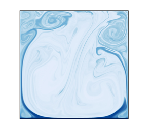
First, the global features of EC turbulence are observed, including the instantaneous and average ones. Some time series samples of the maximum velocity are shown in figure 5. The  $T=700$ case could be regarded as chaos (Zhang et al. Reference Zhang, Chen, Liu, Luo, Wu and Yi2022) while the other cases are all in the EC turbulent regime. Several typical snapshots of the instantaneous charge field and the vorticity denoted by the $Q$ criterion are shown in figure 6, corresponding videos can be viewed in the supplementary material available at https://doi.org/10.1017/jfm.2024.35.

Figure 5. Time series data of maximum velocity at  $T=700$, 3000, 25 000 and 40 000. The blue lines are the temporal evolution of the maximum velocities, the red dashed lines are the temporal average values and the corresponding values are marked near the end of the average value line.

Figure 6. Typical snapshots of instantaneous charge and vorticity  $Q$-criterion field for $T=$ (a,e) 700, (b,f) 3000, (c,g) 25 000, (d,h) 40 000.
The EC turbulence displays pronounced fluctuations as well as strong intermittency. The velocity field evolution shows remarkable differentiation with the change of electric Rayleigh number. For the  $T=700$ case, the value of velocity distributes near the average, and some chaotic, irregular bursts imply a transition of flow structure. Figures 6(a) and 6(e) are typical snapshots in the fluctuation stage. A representative charge void region appears accompanied by a thick charge plume, which rises from the bottom electrode and floats to the upper electrode wall. In the $Q$-criterion contours, vortices are marked by the positive value whereas the viscous stress dominant regions are denoted by negative values. It can be seen that the vortices are more likely to appear near the charge plumes. The oscillations of the side plumes causes fluctuations, whereas the low-frequency but high-amplitude intermittencies come from the variant of flow structures when the central plume appears, and the flow field is reorganized. Previous work also reported similar phenomena (Li et al. Reference Li, Su, Luo and Yi2020; Zhang et al. Reference Zhang, Jiang, Luo, Li, Wu and Yi2023).
For the case  $T=3000$, the velocity fluctuation becomes more frequent and the oscillation amplitude is bigger. Two significant intermittency periods are shown in the time series sample. The typical snapshots are shown in figures 6(b) and 6(f). The central charge plume moves toward the side walls, and the side wall plumes emit more downward dissipative plumes into the charge void region. From the contours of the $Q$ criterion, the vortices at the side walls become stronger. The rolls near the upper corners make the side wall plumes turn towards the central area after reaching the corner areas. The plumes then float downwards, dissipating in the central charge void region.
As shown in figures 6(c) and 6(g), the charge plumes ejected from the bottom wall become slimmer for case  $T = 25\,000$. Almost no plume is released in the bottom electrode's central area (the large-scale turbulent winds push them toward the side walls). Two small rolls appear at the bottom corners and form low charge regions. These two weak rolls are suppressed by the main plumes and hardly develop into bigger structures. In addition, more complicated rolls appear at the upper corners, where the charge plumes are controlled by the rolls, rotating and being propelled towards the big charge void cell. The intermittency in the time series comes from the transition of LSC, causing the charge plume to collapse early before reaching the upper electrode.
For the  $T=40\,000$ case, the highest driven parameter in the current study, the velocity field evolution converts to a different mode. There is almost no increase in the average maximum velocity compared with the large increment in the electric Rayleigh number. The anomalous velocity saturation implies a transition of LSC. In the snapshots in figures 6(d) and 6(h), the main charge plume departs from the side walls and is ejected from the central part of the bottom electrode with a wide plume filament. An extensive roll appears in the central part of the cavity, and multiple small vortices are distributed around the primary roll.
Time-averaged charge fields, velocity fields and pressure fields at  $T =700$, $3000$, 25 000 and 40 000 are shown in figure 7. It is noted that the average fields represent the flow modes that are most likely to occur at distinct driven parameters. The thickness of the charge plumes becomes slimmer with an increase of the $T$ value. Furthermore, the large central charge void regions always exist in each case. It can be concluded that the change in plume thickness stems from the convection effect. It is on account that increasing the $T$ value in a hydrostatics system will not influence the charge distribution when the injection strength $C$ is constant. The average fields show the secondary corner rolls at $T=25\,000$ with lower charge density. The flow structures in the first three cases ( $T=700$, 3000 and 25 000) are like the double rolls mode that has been mentioned several times in previous works (Wu et al. Reference Wu, Traoré, Vázquez and Pérez2013; Pérez et al. Reference Pérez, Vázquez, Wu and Traoré2014; Zhang et al. Reference Zhang, Chen, Liu, Luo, Wu and Yi2022). This mode has the best electric current transport efficiency but is not the most stable one at the flow onset stage in an enclosed cavity with a unit aspect ratio (Pérez et al. Reference Pérez, Vázquez, Wu and Traoré2014).

Figure 7. Time-averaged charge fields (a–d), velocity magnitude with streamline vectors (e–h) and relative pressure field (i–l), the reference point of pressure is chosen at  $(0.5, 0)$ where the relative pressure is always zero. The results for $T=700$, 3000, 25 000 and 40 000 are shown from left to right, respectively.
An interesting change occurs in the pressure fields. The completed pressure in unipolar injection EC consists of the thermodynamic pressure and an extra electrostrictive contribution (Castellanos Reference Castellanos1998; Traoré & Pérez Reference Traoré and Pérez2012; Li et al. Reference Li, Su, Luo and Yi2020), that is,  $p = p_0 - \frac {1}{2}\boldsymbol {\nabla }[\rho \boldsymbol {E}^2 (\partial \varepsilon /\partial \rho )_{\theta }]$, however, the latter is negligible in an incompressible flow. With the increase of $T$, a low-pressure area or even a negative pressure area appears at the central area. The pressure distribution directly causes the velocity field structure, and the fluid is always pushed from the high-pressure area to the low-pressure area. Here the low-pressure area may cause the flow field to redistribute towards the centre, increasing the possibility of LSC transition. It also indicates that the EC turbulence may have more unstable coherent structures and lack a stable LSC for these control parameters.
The  $T = 40\,000$ case is discussed individually because it shows a different average flow mode similar to the single roll mode in the supercritical bifurcation branch (Wu et al. Reference Wu, Traoré, Vázquez and Pérez2013). The charge in the central void region is slightly higher than that at lower $T$ values, and charge plumes do not concentrate in the middle of the upper electrode. The flow structure consists of a big roll that occupies most of the domain and a narrow roll that is usually explained as two secondary vortices. A similar single main roll structure in laminar EC always appears at the flow onset stage, which has a low charge transport efficiency (Wu et al. Reference Wu, Traoré, Vázquez and Pérez2013; Zhang et al. Reference Zhang, Chen, Liu, Luo, Wu and Yi2022). In turbulent EC the mode with a single big roll is also a type of main flow structure. When this mode is dominant, the turbulence results in a relatively low charge transport efficiency that is discussed later. Meanwhile, the negative pressure area also departs from the central region.
6. Charge transfer modes
The current density via the two parallel plates is a measurable variable in the practical experiment. The electric Nusselt number stands for the increment of current contributed from the convection. These two characteristic variables resemble the heat flux and Nusselt number in the RBC. In this section we discuss the evolution of the electric Nusselt number and current density with  $T$, and attempt to reveal the influence of flow modes on the charge transport.
6.1. Electric Nusselt number and charge current
Figure 8(a) shows the temporal average electric Nusselt number, and figure 8(b) illustrates the current (multiplied by coefficient  $T/M^2$). The reason for using the coefficient is that the transformed current is proportional to the practically measured current values, which gives us intuitive and quantitative information contributed by the electric Rayleigh number. We ignore the supercritical bifurcation in the flow onset stage. These maps display the quantity change from hydrostatics to laminar, to chaos (Zhang et al. Reference Zhang, Chen, Liu, Luo, Wu and Yi2022) and then to turbulence states. The obvious increment happens when the subcritical threshold is reached. However, $Ne$ seems to be saturated when the flow enters the chaotic regime. The chaotic flow does not contribute (almost) any increment to the charge transport efficiency shown as the nearly unchanged electric Nusselt number, whereas the increase of current is proportional to the $T$ value. It is shown that the charge transport enters another mode after the flow becomes turbulent. As $T$ ranges from 1500 to 10000, the electric Nusselt number increases following a higher scale law that is nearly approached as $Ne \sim T^{1/2}$. The ${1/2}$ law was first proposed by Lacroix et al. (Reference Lacroix, Atten and Hopfinger1975). Huang et al. (Reference Huang, Wang, Guan, Du, Deepak Selvakumar and Wu2021) also found a scaling law close to the $T^{1/2}$ in a study of EC between concentric cylinders at very high $T$ values and high electric mobilities.

Figure 8. The electric Nusselt number  $Ne$ (a) and dimensionless charge density current $I_e$ normalized by $T/M^2$ (b), where the straight lines represent the approximated scale law $Ne \sim T^{k}$ and $I_e \times T/M^2 \sim T^{k}$, the error bars represent the standard deviation of a time series data set.
Note that the  $1/2$ scaling law observed by Lacroix et al. (Reference Lacroix, Atten and Hopfinger1975) appears before the electric Nusselt number reaches saturation. They supposed the phenomenon happens in an infinite dielectric liquid layer, where EC trends to form self-organizing flow structures without lateral restriction. The stability analysis of EC is also performed based on the length scale, which most easily becomes unstable, namely, the optimal wavelength (Atten & Lacroix Reference Atten and Lacroix1978; Zhang et al. Reference Zhang, Martinelli, Wu, Schmid and Quadrio2015). Nevertheless, there are more complicated behaviours that emerge since the flow is restricted by lateral walls. The side wall limitation lets the flow pattern switch between several modes (Pérez et al. Reference Pérez, Vázquez, Wu and Traoré2014). Here we do not get exactly the $Ne \sim T^{0.5}$ scaling law in the study, but only make an approximate comparison with it. The flow in this stage is close to the flow structure with the best charge transport efficiency. However, the unit aspect ratio used in this numerical domain departs from the optimal wavelength, equaling 1.228, and contains two vertical stacked rolls (Atten & Lacroix Reference Atten and Lacroix1978).
An anomalous  $Ne$ decrease appears when $T$ exceeds 15 000. According to the scaling law derived by Lacroix et al. (Reference Lacroix, Atten and Hopfinger1975), the $Ne$ value remains at saturation at a large enough $T$. Traoré & Pérez (Reference Traoré and Pérez2012) simulated EC at a 0.618 aspect ratio cell and observed the saturation while the case $M=10$ was not considered in their work. The electric Nusselt number decreases quickly with increments of $T$, and the decreasing law seems to be lower than $T^{-1/2}$, the corresponding current increment law is below $T^{1/2}$. Such a phenomenon indicates that the flow transforms into another mode with a lower charge transport efficiency.
6.2. The influence of flow modes on charge transport
We have discussed the evolution of the electric Nusselt number and current in EC turbulence with the variation of  $T$ values. This part will explain the charge transport characteristic at the distinct convection regimes. According to the definition of charge current in (2.13a,b), the charge flux consists of convection, electric drift and diffusion current components. First, we give the temporal evolution series of different current transport mechanisms for cases $T=700$, 4000, 25 000 and 40 000, as shown in figure 9. It can be seen that the fluctuation of the electric drift current is weaker than that of the convection current due to the fact that the strength of the velocity fluctuation in the $y$ direction is stronger than that of the electric field fluctuation. Furthermore, the diffusion component is negligible compared with the former two mechanisms during the entire temporal evolution. For a larger $T$ value, the convection component fluctuation amplitude becomes wider. An interesting phenomenon is that the electric drift flux is always weakened when the convection flux is strengthened, especially when the intermittency is triggered, and vice versa. This is because the convection component is mainly contributed by the charge plumes while the electric drifting component depends on the overall charge density in the bulk. When the strength of the charge plumes is strengthened, the charge density decreases in the bulk area. Because the area of the charge void cell is far larger than that of the plumes, the overall electric drifting current decreases.

Figure 9. Time series of charge current components, where the red, blue and black solid lines represent the electric drift, convection and diffusion components, respectively, and the corresponding dashed lines with identical colour are their time-averaged values. The  $T$ value are 700, 4000, 25 000 and 40 000 from top to bottom.
After obtaining a general impression of the time series of the current, we decided to use the Fourier mode decomposition technique to investigate the underlying temporal current change mechanisms. The Fourier mode decomposition has been widely adopted to study the flow structure (Chandra & Verma Reference Chandra and Verma2011, Reference Chandra and Verma2013; Petschel et al. Reference Petschel, Wilczek, Breuer, Friedrich and Hansen2011; Xi et al. Reference Xi, Zhang, Hao and Xia2016; Wang et al. Reference Wang, Xia, Wang, Sun, Zhou and Wan2018; Chen et al. Reference Chen, Huang, Xia and Xi2019) and the influence of flow modes to the heat transfer efficiency (Wagner & Shishkina Reference Wagner and Shishkina2013; Chong et al. Reference Chong, Wagner, Kaczorowski, Shishkina and Xia2018; Xu et al. Reference Xu, Chen, Wang and Xi2020, Reference Xu, Xu and Xi2023) in 2-D and quasi-2-D square convection cells. Here, a brief introduction is given. Generally, a continuous flow field can be considered as the weighted sum of a series of discrete Fourier modes. A velocity field  $(u,v)$ can be projected onto a series of Fourier basis $(\hat {u}^{m,n}, \hat {v}^{m,n})$ by
 \begin{equation} \left.\begin{gathered} u(x,y,t) = \sum_{m,n}A_{x}^{m,n}(t) \hat{u}^{m,n}(x,y) , \\ v(x,y,t) = \sum_{m,n}A_{y}^{m,n}(t) \hat{v}^{m,n}(x,y) , \end{gathered}\right\} \end{equation}
where the Fourier basis  $(\hat {u}^{m,n}, \hat {v}^{m,n})$ is chosen as
 \begin{equation} \left.\begin{gathered} \hat{u}^{m,n}(x,y) = 2 \sin(m {\rm \pi}x) \cos(n {\rm \pi}y) , \\ \hat{v}^{m,n}(x,y) ={-}2 \cos(m {\rm \pi}x) \sin(n {\rm \pi}y) . \end{gathered}\right\} \end{equation}
Even though the Fourier basis function does not satisfy the no-slip velocity boundary condition, many previous implementations have proven that it can capture the flow features well with an elegant form (Chandra & Verma Reference Chandra and Verma2011, Reference Chandra and Verma2013; Petschel et al. Reference Petschel, Wilczek, Breuer, Friedrich and Hansen2011). The corresponding amplitude of each Fourier mode is calculated by the inner product of the velocity field and Fourier basis thanks to orthogonality,
 \begin{equation} \left.\begin{gathered} A_{x}^{m,n}(t)=( u(x, y, t), \hat{u}^{m,n}(x, y) ) =\sum_{i} \sum_{j} u(x_i, y_j) \hat{u}^{m,n}(x_i, y_j) ,\\ A_{y}^{m,n}(t)=( v(x, y, t), \hat{v}^{m,n}(x, y)) =\sum_{i} \sum_{j} v(x_i, y_j) \hat{v}^{m,n}(x_i, y_j) , \end{gathered}\right\} \end{equation}
where  $( u(x, y, t), \hat {u}^{m,n}(x, y) )$ and $( v(x, y, t), \hat {v}^{m,n}(x, y) )$ denote the inner product of $u$ and $\hat {u}$, $v$ and $\hat {v}$, respectively. The energy of each Fourier mode, which is calculated as $E^{m,n}(t) = \sqrt {[A_{x}^{m,n}(t)]^2 + [A_{y}^{m,n}(t)]^2 }$, denotes the strength of each basis. Here, the $(m,n)$ mode is the flow structure with $m$ and $n$ rolls in the $x$ and $y$ directions, respectively. For example, the first four modes with $m,n \in [1,2]$ are shown in figure 10(a). Four typical instantaneous snapshots of the flow field denoted by streamline and charge at $T=25\,000$ are shown in figures 10(b)–10(e). Although the four fields are not exactly the same as the corresponding Fourier basis, we can say they are dominated by these modes. Then we calculate their instantaneous charge current shown in table 2. The flow field structures indeed influence the different current components in the snapshots. The flow dominated by mode (1,1) with a large primary roll has the lowest convection component, and the two vertical rolls mode (2,1) has optimal charge transport efficiency. Recalling the time-averaged fields in figure 7 and their electric Nusselt number in figure 8, the current transport efficiencies in double vertical rolls mode ( $T=3000 \sim 25\,000$) are also higher than that in the single large roll mode ( $T=40\,000$).

Figure 10. (a) Schematic illustration of the first four Fourier modes (1,1), (2,1), (1,2), (2,2). Four typical snapshots dominated by the four modes at  $T=25\,000$: (b) (1,1), (c) (2,1), (d) (1,2), (e) (2,2).
Table 2. The instantaneous current of the entire domain, and each charge current component of the convection, electric drift and diffusion mechanisms. The indexes are corresponding to the order in figure 10.
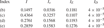
The time evolution of flow structures is more complicated and cannot be described plainly by the instantaneous modes. In the following we consider Fourier modes for  $m,n\in [1, 3]$, namely, the first nine Fourier modes, to study the flow patterns transition. Here, the energy of the $(m,n)$ are normalized by the total energy $E_{total}(t)=\sum _{m,n}E^{m,n}(t)$. We present the time-averaged values of the Fourier mode energy of all cases for $T=700\unicode{x2013} 40\,000$ in figure 11. It can be seen that the (2,1) mode often occupies a dominant percentage. We find that the increase of energy of (2,1) modes is always related to the increase of the electric Nusselt number. There is always a higher charge transport efficiency when there is more flow evolution dominated by (2,1) modes. Besides, figure 11 also shows a competition between the (1,1) mode and (2,1) mode. A decrease of the (1,1) mode percentage corresponds to an increase of that of the (2,1) mode. When the proportion of (2,1) mode reaches the peak, the electric Nusselt number $Ne$ is close to the maximum. It also shows that the modes (1,2), (1,3), (2,2) and (3,1) all have opportunities to have a relatively large percentage (nearly $10\,\%$).

Figure 11. Time-averaged energy of the first nine Fourier modes versus electric Rayleigh number  $T$.
$T$.
In addition, the time evolution of energy percentage in each Fourier mode at  $T=700$, 4000, 25 000 and 40 000 are plotted in figure 12. The energy of (2,1) and (1,1) modes shows an obvious competition from the time evolution, and their proportions always change synchronously, that is, the former increases while the latter decreases at the same time. Combining figure 9, it can be seen that the charge convection flux shares a similar trend with the (2,1) mode during development. When the temporary current is higher than its average value, the flow must be in a (2,1) mode-dominant state. In other words, if the dominated mode is (2,1), the charge transport efficiency is higher, like the regime with a scaling law near $Ne \sim T^{1/2}$ in figure 8(a).

Figure 12. Time evolution of energy in each Fourier mode for (a)  $T=700$, (b) $T=4000$, (c) $T=25\,000$, (d) $T=40\,000$. The legend is only shown in (d) and the other images share the same legend.
The transition of the flow mode is the main reason for the variety of the electric Nusselt number. The competition of various modes causes the electric Nusselt number increment to depart from the optimal scaling law, even to weaken the convection component. From the view of energy transport, a proper moderate-size vertical roll has a higher local velocity, and the upward velocity is close to the walls where the charge plumes tend to attach. This is beneficial for carrying the charge plume to the upper electrode. A large roll that occupies the whole domain has a lower local velocity, and the single circulation must keep similar upward and downward velocities to satisfy mass conservation. Thus, the mass transport efficiency is weaker than the former. In another situation, multiple horizontal rolls are stacked in the vertical direction, making the plumes turn to the central area of the cavity before the plumes reach the upper electrode. These modes also do not reach the best charge transfer efficiency. It lets us recall the flow mode in the study of RBC. The dominant flow mode in RBC is the (1,1) mode, and flow modes with multiple rolls are always the reason for the flow structure transition. However, Xu et al. (Reference Xu, Xu and Xi2023) found that increasing the proportion of (2,1) mode is the most efficient way to improve the heat transfer rate by forcing external shearing. Furthermore, Tsai et al. (Reference Tsai, Daya and Morris2004, Reference Tsai, Daya and Morris2005) derived an analogous  $Nu\sim \mathcal {R}^{\gamma } \mathcal {P}^{\delta }$ scaling (where $Nu$,
$Nu$,  $\mathcal {R}$ and $\mathcal {P}$ are the Nusselt, Rayleigh and Prandtl numbers in their module problem) in annular EC turbulence in which the charge drifting mechanism is subtracted. A fundamental assumption in their derivation is that the turbulent LSCs remain unchanged overall in the unsteady process. This assumption benefits from the natural periodic boundary in the annular geometry. By contrast, the unit square cavity would trigger more flow mode transition in a turbulent evolution. In summary, the reason for the increase, saturation, or decrease of the electric Nusselt number is clarified here with the aid of the Fourier mode decomposition.
7. Mean profiles and energy budget
7.1. Vertical mean profiles
Although the global field features and time evolution reveal many details of the EC turbulence, the distribution of variables between the two electrodes can better express the spatial transport and mass transfer characteristics. The charge and electric field distribution are always the key elements in studying unipolar injection EC. The discussion of the vertical mean profiles begins with these two variables, as shown in figure 13.

Figure 13. Vertical and temporal charge and electric field averages at different  $T$ values. The red lines denote the corresponding distributions for the hydrostatic state. The black dashed lines with markers are 3-D results derived from Kourmatzis & Shrimpton (Reference Kourmatzis and Shrimpton2012).
Figure 13(a) shows the vertical average of the charge for several  $T$ values. The charge decays swiftly at the boundary area $y<0.2$, causing the charge in the bulk to be far below that at the injection electrode surface. The bulk charge increases at $T=30\,000$ and 40 000, indicating the charge in the charge void cell increases slightly at high $T$ turbulence. The charge at the upper wall first increases and then decreases with $T$, reaching its highest value at $T = 10\,000$ in the cases shown. This trend can be explained by the change in the secondary rolls in the upper corners mentioned in § 5. For cases $T<15\,000$, the two big main rolls are relatively stable and rarely stir the corner areas. Thus, the charge void area does not easily reach the upper corners. However, the secondary rolls at the upper corner become more active at higher $T$ values, having more possibilities to mix with the main rolls. Thus, the flow could blend the charge more uniformly. There are a few similarities in the charge distribution at the boundary layer, especially in the region $y<0.1$. An inflection point appears at the charge boundary layers at turbulent regimes, whose position is closer to the wall at a higher $T$ value. The charge boundary layer is similar to the thermal boundary layer in the RBC, which becomes thinner with an increase of the Rayleigh number. Although the increase of $T$ makes the charge boundary thinner, the thinnest charge boundary layer is still in the hydrostatic state. Besides, we compare our results with charge profiles in the 3-D simulation reported by Kourmatzis & Shrimpton (Reference Kourmatzis and Shrimpton2012). Here we choose the S1 and S3 cases ( $R = 1$ and 120) in their work to perform the comparison. Note that the dimensionless mobility $M$ number is different in their study, thus, the discussion could only give qualitative results. Two cases with a similar electric Reynolds number $R$ in the current 2-D study, that is, $T=700$ and 10 000, are chosen for comparison. It shows that the S1 case has an analogous charge density change trend with that of $T=700$, which has a slight increment at the upper electrode. However, the profile of S3 is almost flat near the upper plate, showing a significant difference with case $T=10\,000$. It seems that the 3-D EHD turbulence has a stronger mixing effect. Additionally, the dimensionless ion mobility also influences the turbulent EC but could not be reconciled here.
The average profiles of  $E_y$ are simpler. The electric field distributions do not depart too much from that at the hydrostatic state. The $E_y$ distribution could be simply divided into two regions, one is the boundary layer area in $y = 0\sim 0.1$ and the other is the area from the bulk to the upper electrode. The increase of $T$ makes the electric field boundary layer thinner. Furthermore, the detailed distribution is also different for that at $T<15\,000$ and $T>20\,000$. The former case has a higher electric field strength at the end of the $E_y$ boundary layer. In the bulk area, the distribution of $E_y$ is nearly linear, especially for cases $T>20\,000$. There is a subtle inflection point for the $E_y \vert _{y\approx 0.95}$ at $T <15\,000$, which indicates the upper corner rolls (see figure 7) have a significant effect on the redistribution of potential. Since the dimensionless charge density at $y=0$ is always 1, $E_y \vert _{y=0}$ actually represents the passing current if the diffusion component is neglected. The electric field distribution reveals that the current at $T=10\,000$ is the largest for the cases we have shown.
The contribution of fluctuation variables is discussed next. There are also several works that discuss the relevant terms of fluctuation and the turbulent closure using the higher-order moments (Kourmatzis et al. Reference Kourmatzis, Ergene, Shrimpton, Kyritsis, Mashayek and Huo2012; Kourmatzis & Shrimpton Reference Kourmatzis and Shrimpton2018), whereas we show the fluctuating contribution through the original variables. The corresponding results are shown in figure 14. Except for the chaotic case  $T=700$, the charge fluctuations are significant in the bulk area, even over $60\,\%$ of the average distributions. The charge fluctuations at the upper electrode are also important. The obvious increase of fluctuations always keeps a tiny distance with the injection electrode even at $T=40\,000$. Note that the mean charge density is low in the bulk region, it still needs to be further discussed whether the contribution of charge fluctuation to the flow motion is important although the ratio of charge fluctuation is high here.

Figure 14. The vertical average of the ratio of the fluctuating fields to the temporal average fields: (a) charge, (b) electric field in the  $y$ direction and (c) the ratio of TKE to time-averaged kinetic energy. The charge and electric field averages are represented by their r.m.s. values.
The fluctuation of the electric field seems contrary to the spatial distribution of charge fluctuation, which has a larger proportion near the bottom wall while it is smaller at the bulk area. The fluctuation of the electric field at the bottom electrode, however, does not monotonically change. For example, the fluctuation proportion at  $T=4000$ is higher than that at $T=10\,000$. The proportions of electric field fluctuation are relatively low at $y>0.2$, where they are less than $5\,\%$. The result is consistent with the conclusion derived by Kourmatzis & Shrimpton (Reference Kourmatzis and Shrimpton2012), who analysed the TKE budget and found that the fluctuation of the electric field at the injection electrode could not be ignored.
The comparison of the vertical average kinetic energy and TKE is shown in figure 14(c). The velocity boundary becomes so thin at a high  $T$ value, and the change of kinetic energy could also not be summarized by a monotonous trend. For instance, the proportion of TKE at $T=10\,000$ is even less than that at $T=700$. Figure 14(c) indicates the flow regime at $T=3000 \sim 10\,000$ has a lower turbulent intensity, that is, the LSC is more stable at this regime. It also echoes the possibility of the scaling law we get in figure 8. Because one of the assumptions of the scaling law is that there is a large-scale coherent flow with turbulent wind, the LSC could not be changed frequently. It seems that this stage satisfies the assumption. The TKE proportion is really high at $T >20\,000$, indicating the flow field has a strong fluctuating feature and is mainly governed by the inertial effect.
With the aid of average kinetic energy obtained in (2.16) and (2.20), we discuss the energy budget here. Figure 15 shows the average energy budget for four different cases. The inertial energy is insignificant at  $T=700$, and the energy balance mainly exists between the viscous work and the imported electric power. The inertial energy proportion gets improved at $T=4000$, and the maximum value of viscous work is near the upper wall. For case $T=20\,000$, the inertial energy becomes more important. Furthermore, the viscous work is only dominant near the upper and lower walls. For the case at $T = 40\,000$, in figure 7 we have mentioned the flow structure is changed, and here the profile of inertial work is also diverse from that at $T = 20\,000$. There are multiple peaks of inertial work in the bulk region. The viscous work distribution profile becomes flatter in the bulk area. It is well known that the flow field pattern is directly decided by the pressure distribution and external force if we recall the pressure Poisson equation for the incompressible fluid. Here, the distributions of external force power (that is, $\langle \mathcal {P}_{fe} \rangle _{t,x}$) are similar for all cases, while the pressure power distribution changes significantly. For the inertial force dominant cases $T=20\,000$ and 40 000, in which the inertial term plays a more important role in maintaining the EC turbulence, the curves of these two terms ${\langle \varPi \rangle _{t,x} }$ and ${\langle \mathcal {T} \rangle _{t,x} }$ are nearly identical. When the flow is more dominated by inertial force, the utilization of electric energy is weakened due to the reduced proportion of work done by the electric force. Moreover, the flow patterns become more uncontrollable.


Except for the average kinetic energy transport, we also investigate the fluctuation kinetic energy budget profile to quantitatively understand the intensity and instability of EHD turbulence, as shown in figures 15(e)–15(h). The viscous effect, that is,  $\mathcal {D}_t$ and $\epsilon _t$ terms, always has a dominant effect close to the electrode surface, and the turbulent viscous effect seems more significant in the upper electrode region. When the flow enters the turbulent state, the viscous dissipation in the bulk area is tiny. The convection ${C_t}$ contribution becomes more and more important, even far higher than the contribution of the turbulent electric force power ${\mathcal {P}_{fe,t}}$. The turbulence diffusion ${\mathcal {T}_{t}}$ appears to always maintain a similar proportion in all cases and only consumes a small amount of TKE. Besides, the production of TKE ${\mathcal {P}_k}$ is always transported from the bottom to the top areas. We also compare the TKE budget of $T=700$ to the 3-D case of Kourmatzis & Shrimpton (Reference Kourmatzis and Shrimpton2012) with $T=500$, $R=60$ and $C=10$, and their numerical domain is in horizontal periodic boundaries. The $C_t$, $\mathcal {P}_k$, ${\varPi }_t$, $\epsilon _t$ and $\mathcal {P}_{fe,t}$ terms all share similar trends with the 3-D cases. However, we find that the $\mathcal {T}_{t}$ term has a different distribution between our 2-D results and the cited 3-D case. There is a stronger turbulent dissipation in the 3-D case. We think it is because there is no vortex stretching in 2-D turbulence. It is an essential difference between 2-D and 3-D EHD turbulence. The comparison would give us some qualitative understanding between the 2-D and 3-D EHD turbulence although the driven parameters and boundary are different. Unfortunately, the TKE production and convection transport are ignored in the referred work. It has been shown that these two terms have a significant proportion in 2-D EC turbulence, and we will discuss it in further work.
7.2. Energy box for EC
The so-called energy-box technique is first provided by Ricco et al. (Reference Ricco, Ottonelli, Hasegawa and Quadrio2012) to investigate the energy and enstrophy balances in a channel flow with oscillating walls. Since there is not only a viscous dissipation and electric power balance but also an electric energy transport in a EHD system, we extend the energy-box technique, which only considers the flow system, to the entire EC system. The discussion in this subsection shows the advantages of the energy box for EHD from an overall perspective, pointing out how the evolution of energy proportion changes with the  $T$ values.
Table 3 shows the quantitative dimensionless values of the terms in figure 2. Although the input electric power  $P_{in}$ is two-way coupled with the flow field, values reflect the charge transport ability and the overall power of the system. We list each component of the production of electric force in (2.19) and (2.20). In the time-averaged EHD flow the average power $\langle Q \rangle \langle \boldsymbol {u} \rangle \langle \boldsymbol {E} \rangle$ is dominant, while the fluctuation work represented by the nonlinear terms $\langle q^{\prime } \boldsymbol {e}^{\prime } \rangle \langle \boldsymbol {u} \rangle$ is so small that it can be ignored. There are three components in the electric force production term of the TKE balance equation, i.e. $\langle q^{\prime } \boldsymbol {e}^{\prime } \boldsymbol {u}^{\prime } \rangle$, $\langle q^{\prime } \boldsymbol {u}^{\prime } \rangle \langle \boldsymbol {E} \rangle$, $\langle \boldsymbol {u}^{\prime } \boldsymbol {e}^{\prime } \rangle \langle Q \rangle$. We can see that the terms containing the $\boldsymbol {e}^\prime$ are always small, and only the average electric field has the main contribution of the fluctuating energy production. It also explains why Hopfinger & Gosse (Reference Hopfinger and Gosse1971) thought the $\boldsymbol {e}^\prime$ could be neglected in the average equations. Remember that we have left a question of the effect of $q^{\prime }$ in the discussion of figure 14(a), and now we can explain it. Because the velocity fluctuation is strong enough and cannot be ignored in $\langle q^{\prime } \boldsymbol {e}^{\prime } \boldsymbol {u}^{\prime } \rangle$ and $\langle q^{\prime } \boldsymbol {u}^{\prime } \rangle \langle \boldsymbol {E} \rangle$ terms, the charge fluctuation $q^{\prime }$ is only valuable when it is driven by the mean electric field. Although the fluctuation of the electric field is significant at the injection electrode wall, the fluctuation of charge at the same place is small, so the energy contribution from terms containing $q^{\prime } \boldsymbol {e}^{\prime }$ are tiny. It can be seen that the electric power $P_{fe}$ (that is, the energy that is transported from the electric field to the flow field) decreases after the flow is fully dominated by the inertial effect. The same trend also appears in the change of work contributed by the mean electric field force $\mathcal {P}_{fe,m}$. In contrast, when the increment of $Ne$ reaches the optimal stage, the TKE production $\mathcal {P}_{k}$ decreases, and so does the term $\mathcal {P}_{fe,t}$. We know the flow is dominated by the (2,1) mode in this stage, and the turbulence is organized to be more regular by the electric force, meaning the proportion of TKE energy decreases. The production of TKE and work contributed by fluctuation increases until the $T$ value equals 30 000. We attribute this result to two reasons, one is the flow state transition from the two primary rolls to the single roll mode, and the other is because of the decrease of total input electric power. Figure 11 has shown that the (1,1) mode and (2,1) mode start competing when $T>20\,000$, which makes the flow more stochastic. By associating the energy budgets we present here, we can conclude that the (1,1) mode has a lower energy utilization efficiency.
Table 3. The terms in the energy-box representation and their dimensionless values. For convenience, omit the average angle symbols and factors, here  $\mathcal {P}_{fe,m,1} = \langle Q \rangle \langle \boldsymbol {u} \rangle \langle \boldsymbol {E} \rangle$, $\mathcal {P}_{fe,m,2} = \langle q^{\prime } \boldsymbol {e}^{\prime } \rangle \langle \boldsymbol {u} \rangle$, and $\mathcal {P}_{fe,t,1} = \langle q^{\prime } \boldsymbol {e}^{\prime } \boldsymbol {u}^{\prime } \rangle$, $\mathcal {P}_{fe,t,2} = \langle q^{\prime } \boldsymbol {u}^{\prime } \rangle \langle \boldsymbol {E} \rangle$, $\mathcal {P}_{fe,t,3} =\langle \boldsymbol {u}^{\prime } \boldsymbol {e}^{\prime } \rangle \langle Q \rangle$.

At last, we choose four cases to describe the percentage of each term in the EC systems. For the chaotic state at  $T=700$, the electric field dissipation and the power transported to the flow system occupy half of the total input energy. The portion $\langle \mathcal {P}_{fe,t} \rangle _{V,t}$ shared by the turbulent fluctuation is small. The turbulent energy production $\langle \mathcal {P}_{k} \rangle _{V,t}$ from the mean flow to the fluctuating flow only occupies $0.14\,\%$ of the total power. For case $T=4000$, the fluid system acquires more energy compared with the electric dissipation. The electric force production in the mean flow field allocates $55.66\,\%$ energy and that in the fluctuation field also becomes considerable, that is, $9.14\,\%$, so the proportion of dissipation also increases significantly. The dissipation in the fluctuation field becomes higher than that in the mean field at $T=25000$, it is the feature of strong turbulent flow. The $\langle \mathcal {P}_{k} \rangle _{V,t}$ is also beyond $20\,\%$, which means more energy is sent to the fluctuation and dissipated by it. For case $T=40\,000$, the electric dissipation allocates more input power, indicating the fluid control effect from the electric field is weakened. The TKE production $\langle \mathcal {P}_{k} \rangle _{V,t}$ is also over $22\,\%$. The most shocking result is that the TKE dissipation is nearly four times the MKE dissipation. Although the turbulence intensity is increasing with the $T$ values (refer to the $Re_{RMS}$ number in table 1), it does not mean that the charge transport efficiency in the cavity model will rise. Excessive EC intensity may lead to a shift of the flow pattern, changing the electric force dominant flow into an inertial dominant mode. The latter has a lower energy utilization efficiency and dissipates more energy in the fluctuation. We could conclude that the flow mode with a single large roll, (1,1) mode, is not the optimal mode for charge and energy transport, and is more likely to be dominated by inertial effect. In contrast, the (2,1) mode, which is more controlled by the electric force, prefers to realize more efficient charge transport and energy utilization.
8. Conclusions
This paper presents a comprehensive study from EHD chaos to fully developed turbulence, including instantaneous and mean features, which expands EHD-related insights. There is strong intermittency in EC turbulence. It was found that the evolution of the electric Nusselt number experiences increasing, saturation, and decreasing stages with electric Rayleigh number increases. The primary flow modes in the turbulence are extracted, including a mode with two vertical rolls and another mode with a large single roll. The former has better charge transport and energy utilization efficiency, behaving as a higher electric Nusselt number flow with more energy transported from the electric field to the flow field. The electric field force dominates the former, and the latter is influenced more by inertial effects. The mode with two vertical rolls is related to the  $T^{1/2}$ scaling law reported by Lacroix et al. (Reference Lacroix, Atten and Hopfinger1975). The entire energy transport route from the input electric power to the viscous dissipation is presented using the energy-box technique. When the turbulence reaches the inertial-effect-dominant stage, the fluctuation effects consume more electric energy, decreasing the electric Nusselt number and energy utilization efficiency. The fluctuating electric field $\boldsymbol {e}$ was found to occupy a large proportion near the injection electrode compared with the mean electric field. However, the overall effect of $\boldsymbol {e}$ is negligible because the main contributions of the external force in the mean and fluctuating equations are $\langle Q \rangle \langle \boldsymbol {u} \rangle \langle \boldsymbol {E} \rangle$ and $\langle q^{\prime } \boldsymbol {u}^{\prime } \rangle \langle \boldsymbol {E} \rangle$. The results further confirm the conclusions reported by Hopfinger & Gosse (Reference Hopfinger and Gosse1971) and Kourmatzis & Shrimpton (Reference Kourmatzis and Shrimpton2012). The turbulent diffusion in 2-D turbulent EC is less than that in 3-D turbulence (Kourmatzis & Shrimpton Reference Kourmatzis and Shrimpton2012), probably because there is no vortex stretching in 2-D turbulence, representing an essential difference between 2-D and 3-D turbulence.
This study explores 2-D EC turbulence in an enclosed cavity and performs several comparisons to existing 3-D results. However, there are still numerous characteristics of EHD turbulence that remain to be studied. For example, EC turbulence at different charge injection strengths and mobilities is seldom studied, the  $Ne \sim M^{1/2}$ scaling law (Lacroix et al. Reference Lacroix, Atten and Hopfinger1975) has not been reproduced with certainty, and the large-scale coherent structure of EC turbulence and its influence on charge plumes also deserves additional investigation. Three-dimensional EC turbulence will be further studied in future work. For instance, future studies could concentrate on the EHD energy cascade and the influence of boundary conditions on 3-D EC turbulence. In addition, Fourier mode decomposition and energy-box techniques are considered advantageous for application to future EC studies.
Supplementary movie
Supplementary movie is available at https://doi.org/10.1017/jfm.2024.35.

Figure 16. Energy-box representation for the EC and the energy proportions are marked in each box, (a)  $T=700$, (b) $T=4000$, (c) $T=25\,000$, (d) $T=40\,000$. The term $\langle P_{in} \rangle _{V,t}$ is the whole input electric power supplied to the system, and the terms $\langle P_{visc}\rangle _{V,t}$ and $\langle P_{elec}\rangle _{V,t}$ represent the energy transported to the flow system and dissipated by the electric field. The $\langle \mathcal {P}_{fe,m}\rangle _{V,t}$ and $\langle \mathcal {P}_{fe,t}\rangle _{V,t}$ terms represent the input work by the average flow and the fluctuating flow, the $\langle \epsilon _{m}\rangle _{V,t}$ and $\langle \epsilon _{t}\rangle _{V,t}$ represent the viscous dissipation consumed by the average and fluctuating flow fields, and the $\langle \mathcal {P}_{k}\rangle _{V,t}$ term is the turbulent energy production carried from the average flow to the fluctuating flow.

Figure 17. Probability density functions (p.d.f.s) of the normalized horizontal velocity  $(u_x - \mu _{u_x})/\sigma _{u_x}$ and vertical velocity $(u_y - \mu _{u_y})/\sigma _{u_y}$ measured along the line in the central region $y=0.5$. The left pictures are p.d.f.s at mid-height $0.25 \leqslant x \leqslant 0.75$ and the right pictures are p.d.f.s at the sidewall region, i.e. $0 \leqslant x<0.25$, $0.75< x \leqslant 1$. The black dashed lines represent Gaussian distribution.
Acknowledgements
The authors acknowledge useful discussions with Professor W. Zhao, Northwest University, Xi'an 710127, PR China, and Mr B.-R. Xu, School of Aeronautics, Northwestern Polytechnical University, Xi'an 710127, PR China. Numerical computations were performed on Hefei advanced computing center.
Funding
This work is supported by the National Natural Science Foundation of China (grant no. 52076055) and the Fundamental Research Funds for the Central Universities (grant nos. FRFCU5710051020 and HIT.DZJJ.2023104).
Declaration of interests
The authors report no conflict of interest.
Appendix. Prior validation of 2-D EC turbulence
Probability density functions (p.d.f.s) of the normalized horizontal velocity  $(u_x - \mu _{u_x})/\sigma _{u_x}$ and vertical velocity $(u_y - \mu _{u_y})/\sigma _{u_y}$ measured at the mid-height ( $y=0.5$) are shown in two regions: one is in the central region $0.25 \leqslant x \leqslant 0.75$, and the other is the sidewall region $0 \leqslant x<0.25$, $0.75 < x\leqslant 1$, as shown in figure 17. Here, $\mu$ and $\sigma$ represent the mean value and standard deviation. The EC turbulence is anisotropy because of the existence of an external polar electric field and wall effect. It can be seen that the p.d.f.s of $u_x$ are nearly symmetric at the mid-height. The shapes of all cases follow Gaussian distribution while the tails depart from that, especially for cases $T>1000$. The p.d.f.s of $u_y$ are different. For the central region, we find that the skewness profiles of $u_y$ are large and the main peaks depart from zero. The left part tails of the p.d.f.s are also near the Gaussian distribution whereas the right parts are far away from that. It means that the downward flow appears more easily in this region and the main flow is intermittent. However, the p.d.f.s of $u_y$ in the sidewall region are close to Gaussian distribution, indicating the flow here is random. The left parts of these p.d.f. tails are wider, which means the extreme conditions of downward flow are also likely to appear in this region. From the shapes of the p.d.f.s, it can be concluded that the EC flow is random and clearly intermittent for cases at $T>1000$, matching the features of turbulence. Castellanos (Reference Castellanos1991) proposed that fully developed EHD turbulence should be at a Reynolds number consisting of large-scale eddies $Re \sim O(100)$. Thus, in this work, referring to the cases at $T \geqslant 2000$ as 2-D EC turbulence is reasonable and conservative.


