


1. Introduction
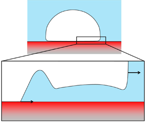
A high heat transfer rate associated with the phase change makes nucleate boiling the most suitable mode of heat transfer in a variety of industrial applications, such as electronics cooling, nuclear power reactors and chemical processes. During the growth of bubbles on a heated wall, a layer of liquid a few  $\mathrm {\mu }$m thick (known as a microlayer) can be formed between the wall and the liquid–vapour interface of the bubble (Bureš & Sato Reference Bureš and Sato2021); cf. figures 1(a,b). Its radial extent on the wall is up to a few mm. Heat is then transferred from the heated wall towards the liquid–vapour interface through the microlayer. The microlayer is a desired feature in boiling heat transfer equipment because it acts as a very efficient heat transfer bridge between the heated wall and the liquid–vapour interface of the bubble, promoting a high heat flux that cools down the heated wall (Kim Reference Kim2009). As the microlayer reduction leads to the dry spot spreading, knowledge of its dynamics is vital for the clear understanding of the boiling crisis that occurs at a critical heat flux, i.e. the maximum heat flux transferrable with nucleate boiling (Zhang et al. Reference Zhang, Wang, Su, Kossolapov, Matana Aguiar, Seong, Chavagnat, Phillips, Rahman and Bucci2023).

Figure 1. Schematics of (a) the general bubble shape, (b) the microlayer geometry, and (c) a liquid layer deposition by dip coating.
Exhaustive information about the microlayer can be obtained only by direct observation. In the past, it was realised with the laser interferometry method in single-bubble experiments (Jawurek Reference Jawurek1969; Voutsinos & Judd Reference Voutsinos and Judd1975; Koffman & Plesset Reference Koffman and Plesset1983; Gao et al. Reference Gao, Zhang, Cheng and Quan2013; Jung & Kim Reference Jung and Kim2015; Chen, Haginiwa & Utaka Reference Chen, Haginiwa and Utaka2017; Zou, Gupta & Maroo Reference Zou, Gupta and Maroo2018; Sinha, Narayan & Srivastava Reference Sinha, Narayan and Srivastava2022).
The pioneering laser interferometry observations (Jawurek Reference Jawurek1969; Katto & Shoji Reference Katto and Shoji1970; Voutsinos & Judd Reference Voutsinos and Judd1975; Koffman & Plesset Reference Koffman and Plesset1983) were realised between the 1960s and 1980s. More recently, there was a resurgence of interest from many research groups (Gao et al. Reference Gao, Zhang, Cheng and Quan2013; Jung & Kim Reference Jung and Kim2015; Zou et al. Reference Zou, Gupta and Maroo2018; Sinha et al. Reference Sinha, Narayan and Srivastava2022) related to the availability of high-resolution fast cameras that provide far better accuracy. The observed microlayer shape depended mostly on the heating mode. In most works the heating was homogeneous, and the observed initial microlayer thickness was a monotonic function of the radial coordinate  $r$ along the heated wall, with origin at the bubble centre. In the experimental approach of Chen et al. (Reference Chen, Haginiwa and Utaka2017), the heating was performed by directing a jet of hot gas to the bottom of the heater, so the heating was localised to a spot smaller than the bubble departure size. In this case, a bump was observed in the microlayer shape. It should be noted that the bump was also observed in some cases at homogeneous heating (Jung & Kim Reference Jung and Kim2018). The origin of this bumped profile has remained largely unexplained.
The physical origin of the microlayer has been studied since the 1960s (Cooper & Lloyd Reference Cooper and Lloyd1969). It was understood that the microlayer appears due to the rapid bubble growth and the inertial force that pushes the bubble towards the wall, thus causing the bubble hemispherical shape. At the same time, viscous and phase change effects affect the microlayer. The semi-empirical formula  $\delta _0\propto \sqrt {\nu t}$ was proposed for the initial microlayer thickness (that at the bubble foot edge; cf. figure 1b), where
  $\nu$ is the liquid kinematic viscosity. A more advanced theoretical approach based on a hydrodynamic analysis of the microlayer was developed later by Smirnov (Reference Smirnov1975). From the fluid dynamics perspective, the microlayer is simply a thin liquid film. It is well known that the flow in thin films is controlled by the surface tension and viscosity only. So the same parameters should primarily control the microlayer dynamics (Katto & Shoji Reference Katto and Shoji1970; Hänsch & Walker Reference Hänsch and Walker2016). A fluid flow exists near the bubble foot edge and near the contact line (CL); the flow in between (where the interface is nearly flat) is extremely weak (Hänsch & Walker Reference Hänsch and Walker2016; Urbano et al. Reference Urbano, Tanguy, Huber and Colin2018; Zhang & Nikolayev Reference Zhang and Nikolayev2021). For this reason, after their formation, the thickness of micrometric films should vary (more precisely, decrease) due to evaporation only.
In the same vein, Zijl & Moalem-Maron (Reference Zijl and Moalem-Maron1978), Brutin, Ajaev & Tadrist (Reference Brutin, Ajaev and Tadrist2013), Schweikert, Sielaff & Stephan (Reference Schweikert, Sielaff and Stephan2019), Kim & Oh (Reference Kim and Oh2021) and Bureš & Sato (Reference Bureš and Sato2021) hypothesised that the microlayer formation, in pool and flow boiling conditions, is analogous to the liquid film deposited during the dip coating when a flat plate is being pulled out vertically from a liquid pool with speed  $U$ (figure 1c). As derived by Landau & Levich (Reference Landau and Levich1942), the film thickness in the limit of low
  $U$ is
 \begin{equation} \delta_0=1.34r_c\,Ca^{2/3}, \end{equation}
where  $r_c$ is the radius of curvature of the liquid meniscus, and
  $Ca=\mu U/\sigma$ is the capillary number. Here,
  $\mu$ and
  $\sigma$ are the liquid shear viscosity and surface tension, respectively. The numerical constant is the same as for a thin film deposited by the meniscus receding in a capillary tube (Bretherton Reference Bretherton1961). This analogy is valid only for a portion of microlayer far from the CL (where the dewetting effects caused by the CL motion are negligible). To the best of our knowledge, there is no direct experimental evidence that a microlayer in nucleate boiling can be seen as the Landau–Levich film.
The objective of this work is to apply a novel – for this domain – experimental technique (Glovnea et al. Reference Glovnea, Forrest, Olver and Spikes2003), the spectrally resolved white-light interferometry (WLI), to show that the microlayer origin is similar to that of the Landau–Levich film, i.e. the initial microlayer thickness  $\delta _0$ of figure 1(b) is defined by (1.1). We also aim to explain the microlayer bumped shape and describe the growth dynamics of the dry spot that forms on the heater under the bubble.
2. Experiment
The experimental cell is filled with water for saturated pool boiling at atmospheric pressure. The bulk liquid temperature is stabilised at  $100\,^{\circ }$C. The experimental set-up (figure 2) is analogous to that of Jung & Kim (Reference Jung and Kim2015) except for the features discussed hereafter. The heater is an indium–tin oxide (ITO) film of thickness
  $h\simeq 950\,{\rm nm}$ deposited on a magnesium fluoride (MgF
 $_2$) optical porthole by using a radio-frequency magnetron sputtering system. The MgF
 $_2$ is transparent to both visible and infrared (IR) waves (95 % transmittance within 0.4–
 $5\,\mathrm {\mu }$m bandwidth), whereas ITO is transparent to visible light but absorbs IR waves. Such a material gives us an enormous advantage of being able to directly measure the wall temperature (i.e. that of ITO). The use of a more conventional (for this field) sapphire would require solving a separate inverse problem (Bucci et al. Reference Bucci, Richenderfer, Su, McKrell and Buongiorno2016), which would introduce a supplementary non-negligible uncertainty. However, during the boiling experiment, the ITO delamination from such a substrate is a tricky issue because of its high coefficient of thermal expansion. The good-quality deposition was mastered by the authors at LPICM.

Figure 2. Experimental set-up and typical images filmed by the cameras. The RTD is a resistance temperature detector.
The growth of a single bubble at a time is performed by using an IR  $1.2\,\mathrm {\mu }$m laser shone to the porthole from below at a single nucleation site found on the ITO surface by its scanning with the laser spot. The laser beam of
  ${\sim }1.5\,{\rm mm}$ diameter is absorbed by the ITO, thus providing its localised heating. The temperature on the ITO surface is a Gaussian-like profile with temperature
  ${\simeq }32$ K at the nucleation site, situating in the centre of the heating spot (figure 2d). The average applied heat flux is 1.1 MW m
 $^{-2}$. The local value at the nucleation spot can be even larger. Three fast cameras synchronised at 4000 fps are used for observation. The first provides the side view shadowgraphy to measure the overall bubble shape, in particular the bubble foot diameter
  $r_b$ (figure 2a). The second camera at the exit of a spectrometer is used for WLI (figure 2c). From this, one can obtain the microlayer thickness
  $\delta (r,t)$, the dry spot (i.e. CL) radius
  $r_{cl}$, and the microlayer radius
  $r_\mu$, within which the interference fringes appear. The WLI is used instead of laser interferometry because it presents several advantages, discussed in the next section. Similarly to Jung & Kim (Reference Jung and Kim2018), the interferometry validation was performed by measuring the profile of the air film formed between a flat surface and a lens of a known curvature (see Appendix A).
The third camera is IR with 3– $5\,\mathrm {\mu }$m bandwidth. It images the IR radiation emitted by the ITO film, thus allowing us to measure its local temperature (figure 2d). Note that besides the WLI image (figure 2c), the microlayer extent is visible both at direct observation from below (figure 2b) and in wall temperature distribution (figure 2d). More details on the experimental set-up are given in Appendix B.
3. Maximum observable interface slope
The vapour–liquid interface slope  $\theta$ is defined from the expression
 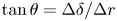 $\tan \theta =\Delta \delta /\Delta r$, where
  $\Delta r$ corresponds to the horizontal distance between the interfacial points, and
  $\Delta \delta$ is determined from the image of interferometry fringes. This distance is related to the distance
  $\Delta r_p$ measured in pixels at the interferometric image (figure 2c) with the relation
  $\Delta r=\mathcal {R}^{-1}\,\Delta r_p$, where
  $\mathcal {R}^{-1}$ is the inverse spatial resolution of the optical system, i.e. the physical size corresponding to 1 px. One deduces that
 \begin{equation} \Delta r_p=\frac{\Delta\delta\,\mathcal{R}}{\tan\theta}. \end{equation}
One can see that for a given  $\Delta \delta$, increase of
  $\theta$ leads to the decrease of
  $\Delta r_p$, so two points can no longer be distinguished if
  $\Delta r_p<1\,{\rm px}$, which results in a limitation for the observable interface slope
  $\theta <\theta _{cr}$, where the critical interface slope is
 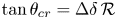 $\tan \theta _{cr}=\Delta \delta \,\mathcal {R}$.
On the other hand, it is well known (Jung & Kim Reference Jung and Kim2015) that the expressions
 \begin{equation} \left.\begin{gathered} 2(hn_{ITO}\cos\alpha_{ITO}+\delta_{N,max} n\cos\alpha)=(N+1/2)\lambda, \\ 2(hn_{ITO}\cos\alpha_{ITO}+\delta_{N,min} n\cos\alpha)=N\lambda \end{gathered}\right\} \end{equation}
are valid for the  $N$th maximum and minimum of intensity of interference patterns (which correspond to the bright and dark fringes) corresponding to the thicknesses
  $\delta _{N,max}$ and
  $\delta _{N,min}$, respectively. Here,
  $\lambda$ is the light wavelength,
  $n_{ITO}$ and
  $n$ are the ITO and liquid refraction indexes, respectively, and
  $\alpha _{ITO}$ and
  $\alpha$ are the refraction angles in the ITO and the liquid. They are kept for generality even though they are both zero in our study as the light incidence is normal; cf. figure 2. According to (3.2), the difference in film thickness between the neighbouring maximum and minimum is
  $\Delta \delta =\delta _{N,max}-\delta _{N,min}=\lambda /(4n\cos \alpha )$. One cannot distinguish the fringes if the neighbouring maximum and minimum are too close, so one can use the last expression in (3.1); the critical interface slope is finally
 \begin{equation} \theta_{cr}=\arctan\frac{\lambda \mathcal{R}}{4n\cos\alpha}. \end{equation}
This limitation applies to both WLI and laser interferometry. In our case, where  $\mathcal {R}^{-1}\simeq 14\,\mathrm {\mu }$m px
 $^{-1}$, we have
  $\theta _{cr}\lesssim 0.4^\circ$, which is quite restrictive. This is not a specific issue of our installation but a very general feature of interferometry studies. For example, the microregion slope measured previously by Jung & Kim (Reference Jung and Kim2015) and Chen et al. (Reference Chen, Hu, Hu, Utaka and Mori2020) is
  $\theta \sim 0.2^\circ$. Note that the absence of fringes within a thin film is significant and means that the slope is larger than critical.
The critical slope is limited by the optical magnification (which defines  $\mathcal {R}$). The microscope used in some earlier studies (where
  $\theta _{cr}$ can be larger) is impossible here because we want to use simultaneously WLI and IR observation. We thus need a space between the objective and the boiling surface to put the beam splitters (the surface should be very close to the microscope objective). The alternative solution used here is a zoom lens with focal length 60 cm. It is difficult to find a larger zoom with the required low level of optical aberrations, both spherical and chromatic.
In all the previous works on microlayers, the thickness was determined by laser interferometry from the interference maxima and minima, i.e. the fringes. This requires knowing the absolute fringe number. However, typically, the slope is large near the CL (Guion et al. Reference Guion, Afkhami, Zaleski and Buongiorno2018; Urbano et al. Reference Urbano, Tanguy, Huber and Colin2018; Bureš & Sato Reference Bureš and Sato2021; Kim & Oh Reference Kim and Oh2021). The first fringes can thus be lost because of the maximum observable slope limitation (3.3), which is likely to induce a systematic error on the thickness determination for all the measured points. Because of this issue, we believe that laser interferometry is not the most adequate method for a reliable measurement of microlayer thickness for nucleate boiling investigations. We use here the spectrally resolved WLI, where such an error is excluded. The thickness at a given point  $r$ is determined by minimising the deviation between the experimental intensity
  $I_{exp}(r, \lambda )$ and the intensity
  $I_{theo}(r, \lambda )$ obtained with the conventional scalar interference theory; see figure 3 and Appendix A. The decisive advantage of WLI with respect to laser interferometry is that it provides a much larger amount of information about the profile that leads to both a higher accuracy and a better microlayer resolution. Indeed, for each
  $r$, WLI provides the number of data points corresponding to the pixels in a column of the WLI image like that in figure 2(c) (1280 in our case) instead of a single number as in laser interferometry. The number of data points corresponds to the number of pixels with fringes, typically much larger than the number of interference maxima and minima visible on a laser interferometry image (cf. figure 10). We evaluated the accuracy
  ${\pm }15\,\textrm {nm}$ of
  $\delta$ determination, while the
  $r$ accuracy (i.e. half-pixel physical size) is
  $7\,\mathrm {\mu }$m.

Figure 3. An example of a fit of the theoretical  $I_{theo}(\lambda )$ profile to the experiment for a fixed
  $r$ resulting in
  $\delta =6.48\,\mathrm {\mu }$m.
Another advantage of WLI is the absence of spurious interference fringes that are often present in laser interference due to a much longer coherence length of the laser in comparison to the white light. In addition, WLI images the film shape directly so it can be evaluated qualitatively in situ. The shape of both the bright and dark fringes in the WLI image (figure 2c) corresponds to  $\delta (r)$ because the expressions (3.2) imply that
  $\delta (r)$ is an increasing linear function of
  $\lambda (r)$ for both maxima and minima of the light intensity. The zoomed in figure 2(e) portion of the fringe pattern in figure 2(c) clearly shows the bumped microlayer profile.
4. Initial microlayer thickness
As mentioned in the Introduction, the main subject of interest is the microlayer evaporation rate. Since the microlayer is extremely thin, the fluid flow is absent in its middle, so at this point,  $\delta$ is assumed to vary because of evaporation only. This assumption will be verified later. Under conventional assumptions (Nikolayev Reference Nikolayev2022) for the description of film evaporation, the energy balance at the interface leads to
 \begin{equation} \mathcal{L}\rho_l\dot\delta ={-}k\,{\Delta T}/{\delta}, \end{equation}
where  $\mathcal {L}$,
  $\rho _l$ and
  $k$ stand for the latent heat, density and thermal conductivity of the liquid, respectively, and the dot means time derivative. Here,
  $\Delta T=T_w-T_{sat}$ is the wall superheating, with
  $T_w$ and
  $T_{sat}$ representing the wall and saturation temperatures, respectively. Equation (4.1) should be solved at each point
  $r$ of the microlayer, resulting in
  $\delta =\delta (r,t)$.
To obtain the solution of (4.1), one needs to know the initial thickness  $\delta _0(r)$, i.e. the thickness right after microlayer formation at a point
  $r$. Cooper & Lloyd (Reference Cooper and Lloyd1969) and later publications assumed that the initial thickness is that at the bubble foot edge (figure 1b). These two definitions are coherent because the microlayer at a point
  $r$ is formed once the bubble edge reaches
  $r$. However, the bubble edge is not defined precisely, and the spatial thickness variation is large in this region. Therefore, rather than measuring
  $\delta _0$ at the edge, we propose reconstructing it from the experimental data. Before discussing the reconstruction, we need to implement the theory for initial microlayer thickness.
4.1. Application of Landau–Levich model
As the microlayer forms during the bubble foot expansion, i.e. the growth of the microlayer extent  $r_\mu =r_\mu (t)$ (figure 1b), one can express
  $\delta _0$ as a function of either the radial distance
  $r$ or the microlayer formation time
  $t=t_\mu (r)$ at the point
  $r$, where
  $t_\mu (r)$ is the function inverse to
  $r_\mu (t)$. This is why Cooper & Lloyd (Reference Cooper and Lloyd1969) give the initial thickness as a function of
  $t$.
$t$.
To complete an analogy between the dip coating and the microlayer formation, one needs to define  $U$ and
  $r_c$ in (1.1) for the microlayer. As its formation can be seen as a film deposited by the receding bubble foot edge, we have
  $U=\dot r_b$ (dot meaning the time derivative); see the analogy between figures 1(a) and 1(c). The meniscus radius of curvature
  $r_c$ (figure 1a) can be associated with that of the bubble foot edge (figure 1c).
Note that  $r_c$ is different from the bubble dome radius
  $r_b$. The bubble foot is flattened due to the inertial forces acting on the bubble downwards during the rapid bubble growth, so that the bubble shape is hemispherical rather than spherical (figure 2a). Therefore, the portion of the bubble interface between the foot and the dome is strongly curved (see figure 1a), thus
  $\beta =r_c/r_b$ is expected to be much smaller than unity. Since
  $r_b$ is the most important characteristic length of the problem, we assume that
  $r_c$ scales with it, so
  $\beta$ is constant in the first approximation. To apply (1.1) to the initial microlayer thickness, the time evolution of
  $r_b$ is required (figure 4). It is obtained experimentally; cf. § 2.

Figure 4. Experimentally measured time evolution of the bubble diameter  $r_b$, microlayer radius
  $r_\mu$ and dry spot (i.e. CL) radius
  $r_{cl}$; for their definitions, cf. figures 2(a,c).
4.2. Reconstruction of initial thickness
One needs now to obtain  $\delta _0$ from the experiment to compare with the above theory. Because of the limitation discussed in § 3,
  $\delta (r,t)$ could be measured only in a short range of
  $r$. In addition, the first time when the fringes were registered was
  $t_f=1.25\,\textrm {ms}$; the corresponding thickness distribution
  $\delta (r,t_f)$ can be found in figure 8(b). The fringes cannot be distinguished between
  $t_\mu$ (time of microlayer formation) and
  $t_f$; they seem blurred. Note that
 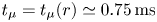 $t_\mu =t_\mu (r)\simeq 0.75\,\textrm {ms}$ in the measurable range of
  $r$ according to figure 4. One can explain the blurring by microlayer dynamics so fast that their displacement is too large during the camera exposure time. This hypothesis is supported by a large
  $\dot r_\mu$ for
  $t\leq t_f$ visible in figure 4. At
  $t\simeq t_f$,
  $\dot r_\mu$ decreases sharply so the fringes are no longer blurred.
To reconstruct  $\delta _0(r)$ from
  $\delta (r,t_f)$, one notes that
  $\delta _0(r)=\delta (r, t=t_\mu )$. One then needs to solve an inverse problem (4.1), where all the parameters are taken for water at atmospheric pressure. One starts by integrating (4.1) from
  $t_\mu (r)$ to
  $t_f$. To simplify the solution, one can use the weakness of both spatial and temporal
  $\Delta T$ variation along the microlayer (figure 5) during the time lapse
  $t_e(r)=t_f-t_\mu (r)\sim 0.5\,\textrm {ms}$; the error introduced by this assumption is minor. We thus use a constant value
  $\Delta T\simeq 6\,\textrm {K}$ (averaged over the time lapse
  $t_e$). Due to this simplification, the result of integration becomes analytical:
 \begin{equation} \delta_{0}(r)=\sqrt{\delta(r,t_f)^2+2k\,\Delta T\,t_e(r)/(\mathcal{L} \rho_l)}, \end{equation}
where the second term inside in the square root represents the thickness of the microlayer that is evaporated during the time lapse  $t_e$. Figure 6 depicts a comparison of
  $\delta _0$ given by (1.1) with the Landau–Levich expression (4.2). The unknown a priori value of
  $\beta =0.084$ is chosen to fit the maximum thickness value. It is remarkable that the position of maximum thickness
  $r\simeq 1.6\,\textrm {mm}$, a key physical feature, is well reproduced by such a simple theory, which supports its validity. Note that the
  $\delta _{0}$ experimental error
  ${\pm }20\,\textrm {nm}$ is slightly larger than that of
  $\delta$ because of reconstruction with (4.2), but it remains much smaller than the symbol height in the inset in figure 6.

Figure 5. The wall superheating variation in the central part of the microlayer where WLI measurements were performed.
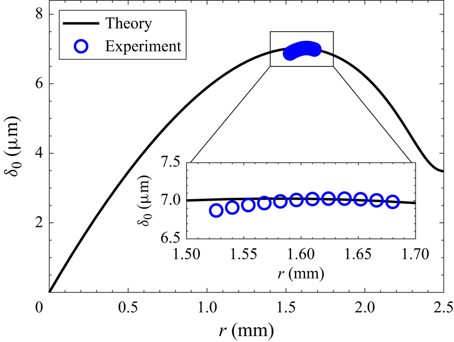
Figure 6. Initial microlayer profile. The experimental WLI data and theory based on (1.1) are compared.
One can now give a simple explanation of the bump. During the microlayer formation,  $U^{2/3}$ decreases in time (in other words, the growth of
  $r_b$ slows down, which is a common feature of the bubble growth; cf. figure 4). At the same time,
  $r_c\propto r_b$ increases. As
  $\delta _0$ is defined by their product according to (1.1), an extremum (i.e. the bump) should appear at some time.
5. Microlayer time evolution and CL dynamics
In the present experiment, the microlayer forms very quickly because of the rapid initial bubble expansion caused by the strongly localised heating. The evolution of the microlayer radius  $r_\mu$, bubble foot radius
  $r_b$ and CL radius
  $r_{cl}$ is presented in figure 4. In the beginning of bubble growth, the microlayer evolves so quickly that it is completely formed at
  $t_f=1.25\,\textrm {ms}$. The CL receding is fast but slower than the
  $r_\mu$ evolution, so the microlayer can form. Until 5 ms, the bubble edge continues to slowly recede (i.e. it moves towards the liquid bulk) so
  $r_\mu$ keeps slowly growing. For
  $5\,\textrm {ms}< t<12.5\,\textrm {ms}$, the bubble edge changes its direction of motion and advances over the microlayer until the latter completely disappears. Note that its disappearance occurs not because of its thickness vanishing caused by evaporation, but because of reduction of its area. Therefore, the term microlayer ‘depletion’, accepted in the boiling community, is hardly adequate. This feature is not specific to the present case; it is commonly observed in the contemporary microlayer studies of pool boiling (Jung & Kim Reference Jung and Kim2018).
In order to interpret and understand the experimental observations, a numerical simulation of the microlayer profile is conducted. In addition to the theory presented in § 4, it accounts for both the CL receding caused by capillary effects amplified by evaporation (Zhang & Nikolayev Reference Zhang and Nikolayev2022) and the microlayer evaporation. The two-dimensional ( $r$–
$r$– $z$; cf. figure 1b) approach (see Appendix C) uses the generalised lubrication approximation. The problem is solved for
  $r\in [r_{cl}, r_b]$, with the end of the interval belonging to the bubble foot edge. The equations and boundary conditions coincide with those of Zhang & Nikolayev (Reference Zhang and Nikolayev2022) except for the boundary condition at
  $r=r_b$. In our case, this condition fixes the curvature to a finite value
  $(\beta r_b)^{-1}$ as in the Taylor bubble problem of Zhang & Nikolayev (Reference Zhang and Nikolayev2021), instead of zero in Zhang & Nikolayev (Reference Zhang and Nikolayev2022). The numerical variation of
  $r_b(t)$ comes from the shadowgraphy measurement (figure 2a);
  $\beta =0.084$ is the result of the fitting performed in § 4.
Our IR thermography measurements reveal a nearly homogeneous temperature over the microlayer extent (Tecchio Reference Tecchio2022), except within the first 0.75 ms. For the simulation, we neglect this non-homogeneity because of its short duration, and impose a uniform  $\Delta T$ over the heater that changes only in time corresponding to the
  $\Delta T_{cl}$ variation at the CL as measured experimentally (figure 5).
The computational algorithm is entirely similar to that of Zhang & Nikolayev (Reference Zhang and Nikolayev2022). The only difference is the use of remeshing at each time step, so the mesh fits the moving boundaries with approximately the same mesh spacing, while the number of nodes decreases. To find the values of  $\delta (t)$ at the node positions corresponding to time moment
  $t+\Delta t$, linear interpolation is used.
The constant physical parameters for water at saturation at 1 bar were taken. The boiling surface was characterised with atomic force microscopy prior to the experiments (figure 7). Beyond the nucleation site, the surface is quite smooth, with roughness  ${\simeq }10\,\textrm {nm}$. It is widely accepted that the hydrodynamic slip length
  $l_s$ corresponds to the roughness (Kunert & Harting Reference Kunert and Harting2007). Therefore,
  $l_s=10\,\textrm {nm}$ was chosen. A reasonable value of the static receding contact angle value
  $10^\circ$ was chosen as
  $\theta _{micro}$ (see Appendix C).

Figure 7. ITO surface imaged by atomic force microscopy (courtesy of C. Rountree). (a) Atomic force microscopy image of the ITO surface. (b) Roughness profile along line AB.
The disjoining pressure is important for the nanometric films. For micrometric films such as a microlayer, it is negligible. Its impact was found to be minor in the CL vicinity for the partial wetting case (Janeček & Nikolayev Reference Janeček and Nikolayev2013; Nikolayev Reference Nikolayev2022).
From the numerical simulation, one obtains both  $U_{cl}$ and
  $\delta (r,t)$ shown in figure 8. The microlayer consists of a ridge located near the CL, followed by a flatter and longer film showing a bumped shape. Consider first the ridge. Its appearance is typical of a dewetting phenomenon (Edwards et al. Reference Edwards, Ledesma-Aguilar, Newton, Brown and McHale2016), i.e. retraction of a liquid film on a non-wettable wall. The dewetting ridge formation is explained as follows. A dry spot and thus CL appear at the nucleation site. Once the microlayer starts to form, the capillary forces tend to reduce the interfacial vapour–liquid area. This effect causes the CL receding that sweeps the liquid previously belonging to the microlayer. At least for the micrometric films (Zhang & Nikolayev Reference Zhang and Nikolayev2022), the net mass of liquid being evaporated in the ridge region is less than the mass of liquid being swept by the CL motion. High viscous stress in the microlayer prevents fluid flow into the film, and the liquid gets accumulated near the CL, thus forming a ridge growing in time. Formation of a dewetting ridge is linked to the CL motion, characterised by the capillary number
  $Ca_{cl}=\mu U_{cl}/\sigma$. The theory of Zhang & Nikolayev (Reference Zhang and Nikolayev2022) shows that it is mainly defined by the wall superheating at the CL
  $\Delta T_{cl}=\Delta T(r=r_{cl})$ presented in figure 9(a). Figure 9(b) illustrates the CL receding. The numerical simulation agrees with the experiment. A strong correlation between
  $Ca_{cl}$ and
  $\Delta T_{cl}$ can be observed, with both featuring a decay over time. One can thus state that the dewetting phenomenon is controlled by the evaporation in the CL vicinity, in agreement with Zhang & Nikolayev (Reference Zhang and Nikolayev2022). The experimental
  $Ca_{cl}$ is approximately 10 times higher at the initial stage of CL receding compared to its final stage. This final
  $Ca_{cl}$ value agrees with the homogeneous wall heating result of Jung & Kim (Reference Jung and Kim2015) shown with a dashed line in figure 9(b). The origin of time decay is the IR laser heating mode, which promotes a highly non-uniform
  $\Delta T(r)$. In the beginning of the evolution, the CL radius is small so it situates at the strongly heated wall part. When the CL recedes, it moves to the colder wall so its speed decreases accordingly.

Figure 8. (a) Temporal evolution of the numerical microlayer profile; see also the supplementary movie available at https://doi.org/10.1017/jfm.2024.488. The corresponding time is labelled in ms. The initial microlayer thickness from figure 6 (given by (1.1)) is also shown. (b) Comparison between numerical simulation (lines) and experimental WLI data (symbols).

Figure 9. (a) Superheating  $\Delta T_{cl}(t)$ measured with the IR camera. (b) Experimental (symbols, obtained from figure 4) and numerical (solid line) evolution of the dimensionless CL speed
  $Ca_{cl}$.
The dewetting ridge is observed in a large majority of bubble growth simulation studies resolving microlayers (Guion et al. Reference Guion, Afkhami, Zaleski and Buongiorno2018; Urbano et al. Reference Urbano, Tanguy, Huber and Colin2018; Bureš & Sato Reference Bureš and Sato2021; Giustini Reference Giustini2024). The essential feature of the present work is that, thanks to the theory of Zhang & Nikolayev (Reference Zhang and Nikolayev2022), we are able to reproduce the CL dynamics. The dewetting ridge was observed for slightly thicker films in another evaporation geometry (Fourgeaud et al. Reference Fourgeaud, Ercolani, Duplat, Gully and Nikolayev2016). One knows that it necessarily occurs at film dewetting, both with evaporation and without (Edwards et al. Reference Edwards, Ledesma-Aguilar, Newton, Brown and McHale2016; Zhang & Nikolayev Reference Zhang and Nikolayev2022, Reference Zhang and Nikolayev2023). However, it has not yet been observed experimentally in boiling. Probably, the reason is the slope limitation of interferometry discussed in § 3. Figure 8 shows that the slopes that occur within the ridge are steep, much steeper than the slope of the remaining microlayer part; the top ridge portion is too small to be detected.
Consider now the remaining microlayer part that forms a bump. Its origin was discussed in § 4. The initial microlayer profile, the same as in figure 6, is displayed in figure 8(a) for comparison. One can see the advantage of the numerical approach over the theory of figure 6: it describes the ridge, the microlayer profile near the CL, and its speed. The simulation also shows the microlayer evaporation corresponding to the thickness reduction, which is nearly uniform, in agreement with the assumption advanced in § 4. One observes a good agreement between the experimental and simulated microlayer shapes in the vicinity of the bump; cf. figure 8(b). In this region, the interface slope is small enough (§ 3) to be measured in our experiment.
Our WLI thickness data of figure 8(b) can seem scarce with respect to those of some other teams, e.g. Chen et al. (Reference Chen, Hu, Hu, Utaka and Mori2020), who recover the full microlayer profile with laser interferometry. However, WLI gives us a much larger density of points (2–7 times larger) and a small uncertainty. The apparent difference between their data and ours can be explained by much stronger pinning of the CL on surface defects in their case, so their receding contact angle is tiny (from their figures,  ${\sim }0.2^\circ$). This hypothesis is supported by their pictures showing a distorted CL (Chen et al. Reference Chen, Hu, Hu, Utaka and Mori2020). In our case, the CL has a nice circular shape (figure 2b) and can advance smoothly (figure 9b) without being pinned, thus indicating a very clean boiling surface of small roughness. Another source of difference is much higher (probably 3–4 times) applied heat flux in our case. The local superheating at nucleation is about 1.4 times higher than for other works (Jung & Kim Reference Jung and Kim2015).
6. Conclusion
In this work, we discuss the physical origin of the microlayer widely observed in nucleate boiling, and apply an advanced experimental method combining three fast optical observation techniques: shadowgraphy, IR thermography, and white light interferometry. The latter is used for the first time in this field of research. We compare it to commonly used laser interferometry. We show that the white-light interferometry is more precise and gives a higher spatial resolution, thus allowing us to have more information about the microlayer. We define the maximum interfacial slope above which the measurements cannot be performed. This limitation applies equally to laser interferometry.
The growth of a single bubble is studied experimentally at pool boiling of water at atmospheric pressure and high surface initial superheating ( ${\sim }30\,\textrm {K}$), not far from that observed at critical heat flux. Such experiments are difficult, as they require extreme purity of water and the absence of defects on the boiling surface, which is the ITO thin film deposited on the MgF
 $_2$ optical porthole. Such a material is advantageous as it is transparent to IR waves, and it is used for the first time in boiling (to our best knowledge). The bubble nucleation and growth are provided by the localised heating with the IR laser.
It is shown that in spite of the inertia-controlled bubble growth and thanks to a tiny thickness of the microlayer, its hydrodynamics is governed by the viscous and surface tension effects. A hypothesis was stated in the literature that the microlayer can be seen as a Landau–Levich film deposited by the bubble foot edge. In this work, we show that the theory based on this hypothesis agrees with the experiment. We introduce a rigorous definition of the initial microlayer thickness. We also explain the origin of the microlayer bump as an interplay of the bubble foot edge curvature and speed of expansion.
We utilise the theory of liquid film dewetting at evaporation to provide an explanation for the expansion of the dry spot beneath the bubble (i.e. the contact line receding). This theory links the receding speed to the local superheating, and exhibits good agreement with our experimental observations. Moreover, this theory predicts the formation of a liquid ridge near the contact line. Although the interferometry studies have not yet captured this liquid ridge due to the limitation of the maximum observable interfacial slope, numerical simulations of several research teams have demonstrated its presence. Since the expansion of dry spot is a crucial aspect in boiling, further experimental ridge studies should be conducted.
Supplementary movie
A supplementary movie is available at https://doi.org/10.1017/jfm.2024.488.
Funding
We are grateful to I. Moukharski, V. Padilla and C. Rountree from SPEC/CEA Paris-Saclay for help with the experiments, and R. Abadie from SPC/CEA for supplying us with the ultra-pure water. C.T. would like to thank DM2S/CEA and the CFR programme of CEA for the financial support of his PhD. X.Z. acknowledges the PhD scholarships of CNES and the CEA NUMERICS programme, which has received funding from the European Union's Horizon 2020 research and innovation programme under grant agreement no. 800945-NUMERICS-H2020-MSCA-COFUND-2017.
Declaration of interests
The authors report no conflict of interest.
Appendix A. The WLI method and its validation
To obtain the microlayer thickness from the spectral fringe map, we use the methodology proposed by Glovnea et al. (Reference Glovnea, Forrest, Olver and Spikes2003), where the function  $F$, defined as
 \begin{equation} F = \sum_{\lambda_{min}\le \lambda \le \lambda_{max}} [I_{c,exp}(\lambda) - \mathcal{K}\,I_{theo}(\lambda)]^2, \end{equation}
is minimised. Here,  $I_{c,exp}(\lambda )$ and
  $I_{theo}(\lambda )$ represent the experimental and theoretical intensity distributions along
  $\lambda$ for a fixed
  $r$. The experimental intensity
  $I_{c,exp}(\lambda )=I_{exp}(\lambda )/I_s(\lambda )$ is compensated to eliminate the effect of uneven spectral intensity emission from the light source;
  $I_{exp}$ is the uncompensated camera output, and
  $I_s(\lambda )$ is obtained from a preliminary experiment at equilibrium with the bare MgF
 $_2$ porthole (without the ITO); and
  $\mathcal {K}$ is a scaling factor that accounts for the different intensity span in the measurements.
The theoretical distribution  $I_{theo}(\lambda )$ is obtained by modelling the intensity of the light that is reflected from the interfaces determined by the MgF
 $_2$, ITO, microlayer and vapour. The transmittance (through the MgF
 $_2$, ITO and microlayer) and the absorbance by the ITO are taken into account by Fresnel equations and a fitting parameter that accounts for the actual light dispersion during the experiment, respectively (Tecchio Reference Tecchio2022).
The  $F$ minimisation is first performed for each point along the
  $r$ axis to get the ITO film thickness. Then
  $I_{c,exp}(\lambda )$ is obtained prior to the bubble nucleation, and
  $I_{theo}(\lambda )$ corresponds to the interference on the ITO film only; its local thickness can be computed with precision at this step. In the second step,
  $\delta$ is determined with a similar minimisation procedure but using the time-dependent fringe pattern
  $I_{c,exp}(\lambda )$ obtained during the bubble growth (figure 2c), while
  $I_{theo}(\lambda )$ (Tecchio Reference Tecchio2022) corresponds to the interference on both the ITO film and the microlayer. They are both functions of already known ITO thickness and
  $\delta$. For each
  $x$, the
  $F$ minimisation gives the
  $\delta$ value.
The set-up was validated by using the plano-convex lens with radius of curvature  ${\rm R}$ given by the manufacturer. The lens was posed on the porthole with a convex side downwards, thus forming an air layer of thickness
  $\delta (r)$. Its theoretical value can thus be determined from the equation
 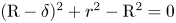 $({\rm R}-\delta )^2+r^2-{\rm R}^2=0$, where
  $r$ is the horizontal coordinate axis on the porthole centred at the point of symmetry of the lens. The experimental data agreed with this theoretical value within 40 nm between 0.1 and
  $6\,\mathrm {\mu }$m; cf. figure 10 (which is a much better agreement than that of Jung & Kim (Reference Jung and Kim2018), where laser interferometry was used).

Figure 10. Comparison of laser interferometry and WLI for the validation case of measurement of the profile of the air film between the ITO surface and a spherical lens posed on it. The theoretical film profile is calculated from the known lens curvature.
The spectral interference patterns (figure 2c) obtained by WLI were compared with those predicted by the theory (Tecchio Reference Tecchio2022). Good agreement was obtained thanks to detailed and rigorous optical alignment and calibration protocols, absence of spurious interference (arising from thicker optical elements or light dispersion), and negligible optical aberrations, both chromatic and geometric.
Appendix B. Details of the experimental set-up
The boiling cell is filled with ultra-pure water treated with Millipore Milli-Q Integral 5 apparatus and thermally regulated at  $100\,^\circ$C with a heating jacket connected to the oil thermal bath. A resistance temperature detector (RTD) is placed inside the water pool to monitor the liquid temperature; the experiment can be started only after several hours of temperature equilibration. Four lateral transparent portholes provide a means for the side view shadowgraphy performed with a Photron SA3 fast camera and telecentric collimated LED light source (Opto Engineering LT CL HP 024-W) positioned at opposite sides of the cell. The growth of a single bubble at a time is triggered by using a continuous-wave IR laser (Changchun New Industries Optoelectronics FC-W-1208B-10W).
The heart of the installation is WLI. A collimated LED white-light source (Thorlabs Solis-3C) illuminates the fluid from below. The waves reflected from the liquid–vapour, liquid–ITO and MgF $_2$–ITO interfaces interfere. They are captured by the 150–600 mm focal length objective (Sigma F5-6.3 DG OS HSM Contemporary) installed at the entrance of a spectrometer (Horiba iHR550) with a fast high-resolution camera (Phantom v2011) at its exit. The spectrometer can function in two modes. In WLI mode, a thin slit at the entrance of the spectrometer defines a scanning line that (due to the in situ adjustment) passes through the bubble centre so its direction defines the radial
  $r$-axis for the bubble. The light arriving from the slit is dispersed by a diffraction grating inside the spectrometer, producing a spectral fringe map captured by the camera. One obtains an intensity distribution
  $I_{exp}(r,\lambda )$ of the fringe pattern (figure 2c), where the ordinate axis in the figure represents the wavelength
  $\lambda$, and the abscissa is the coordinate
  $r$. Both axes are calibrated in situ. This is especially important for the
  $\lambda$ axis as the camera is greyscale. The axial symmetry of fringes is checked carefully. It is provided by the bubble symmetry.
In the direct observation mode of the spectrometer, the slit is fully opened and the diffraction grating in the optical path is replaced with a mirror. One obtains the two-dimensional liquid–vapour distribution on the bubble base (figure 2b) thanks to the difference in refraction indices. Both the dry spot and microlayer can be observed directly to check their circular symmetry.
The IR radiation emitted by the ITO is captured by the IR camera (FLIR X6901sc) operating in the 3– $5\,\mathrm {\mu }$m bandwidth. The camera images the IR radiation emitted directly by the ITO (figure 2d) as MgF
 $_2$ is transparent in this bandwidth. The intensity of radiation is related to the wall temperature through the in situ pixel-wise calibration (Schweikert, Sielaff & Stephan Reference Schweikert, Sielaff and Stephan2021). The visible-IR beam splitter (hot mirror) is transparent to visible light but almost completely reflects the IR waves in the 3–
 $5\,\mathrm {\mu }$m bandwidth. It was designed and produced by the authors as such a device is not available for retail. The hot mirror was qualified by Fourier transform infrared spectroscopy (FTIR).
Appendix C. Generalised lubrication approach
The problem is described in the two-dimensional cross-section of the microlayer (figure 1b). It uses the ‘one-sided’ formulation (Burelbach, Bankoff & Davis Reference Burelbach, Bankoff and Davis1988), where the vapour-side hydrodynamic stress and the heat flux into the vapour at the interface are neglected compared to those on the liquid side. Therefore, the vapour pressure  $p_v$ is assumed to be spatially homogeneous. The heater is highly conductive and thus assumed to be isothermal.
As the interface slope increases considerably in the presence of evaporation, the conventional lubrication theory, valid for slopes below  ${\sim }30^\circ$, becomes insufficient. The generalised lubrication theory (Zhang & Nikolayev Reference Zhang and Nikolayev2022) is used to describe the thin film flow and free liquid–vapour interface of local height
  $\delta (r,t)$. The theory uses the parametric interface description in terms of the curvilinear coordinate
  $s$ that runs along the interface (figure 1b), with
  $s=0$ at the CL. Therefore, the following geometrical relations hold:
 \begin{equation} {\partial\delta}/{\partial s}=\sin\theta,\quad {\partial r}/{\partial s}=\cos\theta, \end{equation}
where  $\theta$ is the local interface slope. The major convenience of this parametrisation is the simplicity of rigorous expression for curvature
  $K$:
$K$:
 \begin{equation} K=\frac{\partial\theta}{\partial s}=\frac{1}{\cos\theta}\,\frac{\partial^2\delta}{\partial s^2}. \end{equation}
The generalised lubrication theory approximates the liquid pressure  $p_l$ by the pressure created by the flow in the straight liquid wedge with opening angle
  $\theta$. The corresponding arc with length
  $\zeta =\delta \theta /\sin \theta$ is defined.
The interfacial pressure jump
 \begin{equation} \Delta p\equiv p_v-p_l=\sigma K -{J^2}(\rho_v^{{-}1} -\rho_l^{{-}1}) \end{equation}
accounts for the vapour recoil effect, where  $\rho _v$ is the vapour density,
  $K$ can be expressed with (C2), and
  $J$ is the local mass flux, assumed positive at evaporation.
Because the liquid films are thin, heat conduction is the main energy exchange mechanism, which can be taken as stationary due to their low thermal inertia. The liquid temperature is assumed to vary linearly along the arc  $\zeta$ from
  $T_w$ to
  $T^i$, as suggested by the rigourous thermal analysis of straight wedges where the heat flow is radial (Anderson & Davis Reference Anderson and Davis1994). The heat flux supplied to the vapour–liquid interface is spent to vaporise the liquid. Therefore, the energy balance at the interface reads
 \begin{equation} J = {k(T_w-T^i)}/({\zeta \mathcal{L}}). \end{equation}
The interfacial temperature  $T^i$ is affected by the Kelvin, vapour recoil and molecular-kinetic effects (Carey Reference Carey2020):
 \begin{equation} T^i = T_{sat}[1 + {\Delta p}/({\mathcal{L}\rho_l}) + {J^2}(\rho_v^{{-}2} -\rho_l^{{-}2})/({2\mathcal{L}})] + R^i J \mathcal{L}, \end{equation}
where
 \begin{equation} R^i =\frac{T_{sat}\sqrt{2{\rm \pi} R_v T_{sat}}\,(\rho_l-\rho_v)}{2 \mathcal{L}^2\rho_l\rho_v} \end{equation}
is the kinetic interfacial thermal resistance, with the accommodation coefficient assumed to have value 1 (Eames, Marr & Sabir Reference Eames, Marr and Sabir1997). Here,  $R_v$ is the specific gas constant for the vapour.
The governing equation
 \begin{align} \dot\delta\cos\theta +\frac{\partial}{\partial s}\left\{\frac{1}{\mu\,G(\theta)} \left[\frac{\zeta}{2}\,(\zeta + 2 l_s)\,\frac{\partial\sigma}{\partial s}+ \frac{\zeta^2}{3}\,(\zeta+3l_s)\,\frac{\partial\Delta p}{\partial s}\right] - {U_{cl}}\,\zeta\,\frac{F(\theta)}{G(\theta)}\right\} ={-}\frac{J}{\rho_l} \end{align}
is written in the frame of reference of the CL, which is receding at speed  $U_{cl}$. Here,
  $l_s$ is the hydrodynamic slip length introduced with the Navier slip boundary condition at the wall.
Since the interface temperature  $T^i$ varies spatially (cf. (C5)), the Marangoni term should be included:
 \begin{equation} {\partial\sigma}/{\partial s}\simeq{-}\gamma\,{\partial T^i}/{\partial s}, \end{equation}
where  $\gamma =-\partial \sigma /\partial T$ is generally positive. The functions (Boender, Chesters & van der Zanden Reference Boender, Chesters and van der Zanden1991; Mathieu Reference Mathieu2003)
 \begin{equation} F(\theta)=\frac{2\theta^2}{3}\,\frac{\sin{\theta}}{\theta-\sin\theta\cos\theta} \end{equation}
and
 \begin{equation} G(\theta)=\frac{\theta^3}{3}\,\frac{4}{\sin\theta\cos\theta-\theta\cos 2\theta} \end{equation}
are the correction factors. With  $F(\theta \to 0)=1$ and
  $G(\theta \to 0)=1$, this formulation reduces to the conventional lubrication theory.
Another equation determines the CL speed  $U_{cl}$ (which is a part of the problem). The relation between
  $U_{cl}$ and the evaporation flux at the CL (Zhang & Nikolayev Reference Zhang and Nikolayev2022) is
 \begin{equation} J(s\to 0)=\frac{U_{cl}\,F(\theta_{micro})}{\dfrac{G(\theta_{micro})}{\theta_{micro}\,\rho_l}+ \dfrac{l_s\mathcal{L}\,\theta_{micro}}{\mu k}\,\gamma}. \end{equation}
The governing equations (C7) are solved for  $s\in [0, s_e]$, with a point
  $s_e$ belonging to the bubble foot edge that situates at a horizontal distance
  $r_e\equiv r(s_e)=r_b-r_{cl}$.
As the set of governing equations (C3) and (C7) is of fourth order in  $s$, four boundary conditions should be defined. At the CL (
 $s=0$), the geometry implies
 $$\begin{gather} \delta = 0, \end{gather}$$
 $$\begin{gather}{{\partial \delta }}/{\partial s}= \sin\theta_{micro}, \end{gather}$$
where  $\theta _{micro}$ is the microscopic contact angle controlling the wetting conditions. Its choice is discussed below. One more boundary condition expresses the solution regularity, in particular, the pressure finiteness:
 \begin{equation} {{\partial \Delta p}}/{\partial s}|_{s \to 0}= 0. \end{equation}
The fourth boundary condition fixes the curvature to that of the bubble foot:
 \begin{equation} K |_{s=s_e}= r_c^{{-}1}. \end{equation}
However, one more condition is necessary for matching the microlayer to the bubble edge contour, i.e. the height  $\delta _e\equiv \delta (s_e)$ at which the matching is performed. From the physical point of view, the flows in the microlayer created by the ridge and bubble edge displacements are decoupled from each other because of the quasi-absence of flow in between. A multitude of profiles are thus possible for the given four boundary conditions. The fifth condition is thus needed to select a unique profile. The value of
  $\delta _e$ should be much larger than the microlayer thickness (to provide the curvature saturation) but not too high, to avoid the unrealistic interfacial slopes
  ${\gg }90^\circ$ that can appear because of the constant-curvature boundary condition. We set
  $\delta _e(t)\simeq 0.3r_c$.
Thanks to the curvature saturation at  $s\to s_e$, the solution is quite insensitive to the
  $s_e$ value. For this reason, instead of its self-consistent determination, we use the following approximate procedure. First, we mention that
  $\dot r_e=U-U_{cl}$, where
  $U=\dot r_b(t)$ is obtained from the experimental data, and
  $U_{cl}$ is the CL speed to be determined as part of the solution. Finally, as the point (
 $r_e,\delta _e$) belongs to the hemispherical bubble interface, one can approximately convert the changes in
  $r_e$ and
  $\delta _e$ into the change of
  $s_e$ as
  $\dot s_e= \sqrt {\dot r_e^2 + \dot \delta _e^2}$.
One needs now to choose  $\theta _{micro}$. One knows that
  $U_{cl}$ is controlled mainly by the superheating
  $\Delta T_{cl}$ at the CL, and to a lesser extent by
  $\theta _{micro}$ (Zhang & Nikolayev Reference Zhang and Nikolayev2022). The dependence on the film thickness
  $\delta _\infty$ far from the ridge (assumed constant) is weak (logarithmic). One can superpose the
  $U_{cl}$ experimental data as a function of
  $\Delta T_{cl}$ on the respective theoretical curves obtained with the method of Zhang & Nikolayev (Reference Zhang and Nikolayev2023) for different
  $\theta _{micro}$ (figure 11). One can see that the data are grouped around the curve for
  $10^\circ$, which suggests this value for
  $\theta _{micro}$.

Figure 11. Plots of  $Ca_{cl}$ versus
  $\Delta T_{cl}$. The lines correspond to the theory (Zhang & Nikolayev Reference Zhang and Nikolayev2023) applied to water for different values of the microscopic contact angle
  $\theta _{micro}$ (shown in the graph) and for
  $\delta _\infty =6\,\mathrm {\mu }$m, while the circle symbols are the experimental points.


 Open access