


Nomenclature
- $T$
$T$
-
temperature
-
$E$
-
energy
-
$q$
-
heat flux
-
$p$
-
pressure
-
${p_b}$
-
backpressure
-
$\rho $
-
density
-
$\tau $
-
viscous stress tensor
-
$\mu $
-
dynamic viscosity
-
$\gamma $
-
specific heat ratio
-
$t$
-
time
-
${t_0}$
-
backpressure duration
-
$u$
,
$v$
,
$w$
-
velocity
-
${\delta _{99}}$
-
boundary layer thickness
-
$\theta $
-
momentum thickness
-
$x$
,
$y$
,
$z$
-
coordinates
-
$L$
-
pipe length
-
$H$
-
pipe height
-
$\sigma $
-
impact factor
-
$Ma$
-
Mach number
-
$Re$
-
Reynolds number
-
$Pr$
-
Prandtl number


Subscripts
-
$i$
,
$j$
,
$k$
-
indices
-
$a$
-
condition at shock train leading edge
-
$b$
-
condition at outlet
-
$c$
-
steady state
-
$l$
-
laminar
-
$t$
-
turbulent


Superscripts
-
${}^{*}$
-
total parameter

1.0 Introduction
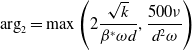
Pulse detonation ramjet (PDR) is a propulsion form using pulse detonation combustion, as shown in Fig. 1. Although most research on PDR focuses on propulsion [Reference Zvegintsev, Ivanov, Frolov, Shamshin and Zangiev1, Reference Ivanov, Frolov, Zangiev, Zvegintsev and Shamshin2] or combustion [Reference Frolov, Shamshin, Kazachenko, Aksenov, Bilera, Ivanov and Zvegintsev3], little work has addressed the shock train in the isolator. The experimental results of a combined aero-valve for a pulse detonation engine show that the supersonic incoming flow in the isolator is a key factor in achieving complete isolation of the backpressure waves [Reference Lu, Zhang, Tan and Zheng4], which means that the shock isolator is an indispensable component of PDR. Furthermore, Studies have shown whether PDR can achieve the efficiency equivalent to the Brayton cycle largely depends on whether the intake system can minimise the total pressure loss [Reference Qiu, Xiong and Li5]. However, the dynamic characteristics, streamwise length, static pressure recovery and the total pressure recovery characteristics of the shock train in the isolator are still poorly understood, which will bring difficulties to the performance analysis and design of the isolator. Therefore, a more thorough investigation is highly needed in this research field. The problems faced by PDR are similar to those faced by scramjet in subsonic combustion mode. Both need to slow down the supersonic incoming flow to subsonic speed and can adapt to the change of the combustor’s backpressure to prevent it from affecting the normal operation of the inlet [Reference Gerdroodbary6, Reference Gerdroodbary7]. The difference between PDR and scramjet is that the peak value of pulse backpressure in a PDR combustor is significant, and the frequency is high. Since there is almost no research on the PDR isolator, the following will introduce the relevant research on the impact of backpressure on the shock train in the isolator of scramjet.
The shock train is a flow phenomenon that occurs during the deceleration of the supersonic flow in ducts, resulting from the interaction between shock waves and boundary layers within a confined space [Reference Matsuo, Miyazato and Kim8]. This phenomenon is commonly observed in various fluid devices, including supersonic inlets [Reference Chyu, Kawamura and Bencze9–Reference Sajben, Donovan and Morris11], diffusers of supersonic wind tunnels [Reference Matsuo, Sasaguchi, Mochizuki and Takechi12] and nozzles [Reference Keanini, Tkacik, Srivastava, Thorsett-Hill and Tomsyck13–Reference Islam, Abir and Hasan15]. In the isolator of the ramjet, the shock train plays a critical role in providing entrance conditions for the combustion chamber and preventing pressure disturbances in the combustor from affecting the upstream flow [Reference Waltrup and Billing16]. The isolator is a section of airflow channel between the combustor and the inlet, which provides a flow space for the formation of the shock train to achieve mode conversion and continues the compression effect to make the incoming flow match the inlet conditions of the combustor. A well-designed isolator should shorten the length as much as possible and improve the total pressure recovery based on meeting the flow conditions required at the inlet of the combustor. The stream-wise size and the aerodynamic performance of the isolator are determined to a great extent by the nominal length, static pressure recovery and total pressure recovery of the shock train [Reference Heiser, Pratt, Daley and Mehta17, Reference Billing18]. As a result, this specific flow phenomenon has gained increasing attention from researchers. Later, researchers found that most influencing factors cannot be maintained at constant levels in an operating engine, and a change in any such factor can lead to unsteady movements in the shock train [Reference Chang, Li, Xu, Bao and Yu19, Reference Sekar, Karthick, Jegadheeswaran and Kannan20]. The most crucial factor is the pressure in the combustor. The shock train oscillation, induced by backpressure disturbances from pulse combustion, posed a significant risk to inlet stability and engine operation. Therefore, scholars extensively investigated shock train oscillations.
In experimental research, perturbational backpressure is typically applied by periodically changing the outlet area of the isolator through the mechanically actuated block [Reference Cheng, Wang and Cheng21, Reference Wang, Chang, Li, Chen, Hou, Guo and Yue22]. Although this method can accurately control the disturbance frequency, it fails to control the backpressure peak directly. In the numerical study, perturbational backpressure can be precisely controlled by using a given function [Reference Hamed and Shang10, Reference Islam, Abir and Hasan15, Reference Gillespie and Sandham23, Reference Peng, Fan, Zheng, Wang and Yuan24]. However, the backpressure simulated in these studies is typically at the level of a scramjet combustor. For example, the backpressure peak in Ref. (Reference Gillespie and Sandham23) is two times larger than that of the inlet, and the oscillation frequency in Ref. (Reference Sethuraman, Kim and Kim25) ranges from 10 to 50Hz. This type of backpressure has a small amplitude and long duration. It differs significantly from the large amplitude and short-duration perturbational backpressure observed in PDRs. In PDR isolators, the pressure gain in the combustor caused by detonation often reaches 5–10 times the upstream pressure, and the working frequency is typically above 100Hz [Reference Peng, Fan, Zheng, Wang and Yuan24, Reference Matsuoka, Muto, Kasahara, Watanabe, Matsuo and Endo26]. Considering the parallels in objectives and principles, the experience garnered from scramjet isolator offers valuable guidance for PDR isolator design. However, full applicability is limited. Thus, investigating flow characteristics and shock train length with the isolator under significant, high-frequency fluctuating backpressure is crucial. This endeavor establishes a theoretical foundation for PDR isolator design.
The current paper presents the simulation results of a shock train in a straight pipe under pulse backpressures of different amplitudes and durations, and the instantaneous distributions of the flow field are analysed. By fitting the amplitude, duration of the backpressure and maximum backpropagation in the tube, an expression describing the relationship between them is obtained. The objectives of this study are to establish a preliminary knowledge of the behaviour of the shock train in a straight pipe under large amplitude and fast impact backpressure and provide a basic comparison with that in a straight pipe under steady backpressure to obtain a prediction formula for the maximum backpropagation distance within the isolator under pulse backpressure.
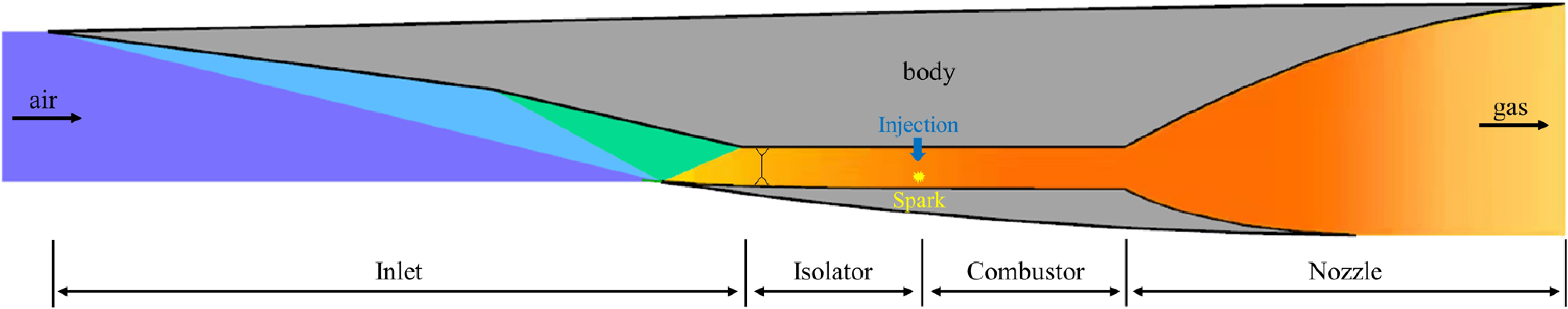
Figure 1. General structure of PDR.
2.0 Numerical methodology and validation
2.1 Methodology
By rendering the governing equation dimensionless through inlet height, dynamic viscosity and density, the variable count is reduced [Reference Gerdroodbary, Moradi and Babazadeh27, Reference Du, Al-Rashed, Gerdroodbary, Moradi, Shahsavar and Talebizadehsardari28]. This equation can be described by
 \begin{align}\frac{{\partial \boldsymbol{Q}}}{{\partial t}} + \frac{{\partial \boldsymbol{E}}}{{\partial x}} + \frac{{\partial \boldsymbol{F}}}{{\partial y}} + \frac{{\partial \boldsymbol{G}}}{{\partial z}} = \frac{{\partial {\boldsymbol{E}_\upsilon }}}{{\partial x}} + \frac{{\partial {\boldsymbol{F}_\upsilon }}}{{\partial y}} + \frac{{\partial {\boldsymbol{G}_\upsilon }}}{{\partial z}}\end{align}
where $\boldsymbol{Q}$
is a conserved variable.
$\boldsymbol{Q}$
is a conserved variable. $\boldsymbol{E}$
,
$\boldsymbol{E}$
, $\boldsymbol{F}$
, and
$\boldsymbol{F}$
, and $\boldsymbol{G}$
are, respectively, inviscid fluxes in the
$\boldsymbol{G}$
are, respectively, inviscid fluxes in the $x$
,
$x$
, $y$
, and
$y$
, and $z$
directions. The specific expressions are given by
$z$
directions. The specific expressions are given by
 \begin{align}\boldsymbol{Q} = \left( \begin{array}{c}\rho \\[3pt]\rho \boldsymbol{u}\\[3pt]\rho \boldsymbol{v}\\[3pt]\rho \boldsymbol{w}\\[3pt]\rho e\end{array} \right)\quad \boldsymbol{E} = \left( \begin{array}{c}\rho \boldsymbol{u}\\[3pt]\rho {\boldsymbol{u}^2} + p\\[3pt]\rho \boldsymbol{uv}\\[3pt]\rho \boldsymbol{uw}\\[3pt](\rho e + p)\boldsymbol{u}\end{array} \right)\quad \boldsymbol{F} = \left( \begin{array}{c}\rho \boldsymbol{v}\\[3pt]\rho \boldsymbol{uv}\\[3pt]\rho {\boldsymbol{v}^2} + p\\[3pt]\rho \boldsymbol{vw}\\[3pt](\rho e + p)\boldsymbol{v}\end{array} \right)\quad \boldsymbol{G} = \left( \begin{array}{c}\rho \boldsymbol{w}\\[3pt]\rho \boldsymbol{uw}\\[3pt]\rho \boldsymbol{vw}\\[3pt]\rho {\boldsymbol{w}^2} + p\\[3pt](\rho e + p)\boldsymbol{w}\end{array} \right)\end{align}
 \begin{align*}{\boldsymbol{E}_\upsilon } = \left( \begin{array}{c}0\\[3pt]{\tau _{xx}}\\[3pt]{\tau _{xy}}\\[3pt]{\tau _{xz}}\\[3pt]\boldsymbol{u}{\tau _{xx}} + \boldsymbol{v}{\tau _{xy}} + \boldsymbol{w}{\tau _{xz}} - {q_x}\end{array} \right)\end{align*}
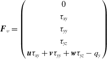 \begin{align*}{\boldsymbol{F}_\upsilon } = \left( \begin{array}{c}0\\[3pt]{\tau _{xy}}\\[3pt]{\tau _{yy}}\\[3pt]{\tau _{yz}}\\[3pt]\boldsymbol{u}{\tau _{xy}} + \boldsymbol{v}{\tau _{yy}} + \boldsymbol{w}{\tau _{yz}} - {q_y}\end{array} \right)\end{align*}
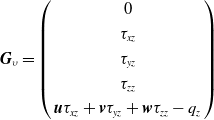 \begin{align*}{\boldsymbol{G}_\upsilon } = \left( \begin{array}{c}0\\[3pt]{\tau _{xz}}\\[3pt]{\tau _{yz}}\\[3pt]{\tau _{zz}}\\[3pt]\boldsymbol{u}{\tau _{xz}} + \boldsymbol{v}{\tau _{yz}} + \boldsymbol{w}{\tau _{zz}} - {q_z}\end{array} \right)\end{align*}
where $\rho $
,
$\rho $
, $p$
, and
$p$
, and $e$
are the density, pressure and total internal energy per unit mass of gas, respectively.
$e$
are the density, pressure and total internal energy per unit mass of gas, respectively. $\boldsymbol{u}$
,
$\boldsymbol{u}$
, $\boldsymbol{v}$
and
$\boldsymbol{v}$
and $\boldsymbol{w}$
, are the velocity components in the
$\boldsymbol{w}$
, are the velocity components in the $x$
,
$x$
, $y$
and
$y$
and $z$
directions, respectively.
$z$
directions, respectively. $\gamma $
is the specific heat ratio. The pressure is given by the ideal gas state Equation (3).
$\gamma $
is the specific heat ratio. The pressure is given by the ideal gas state Equation (3).
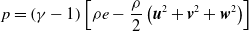 \begin{align}p = \left( {\gamma - 1} \right)\left[ {\rho e - \frac{\rho }{2}\left( {{\boldsymbol{u}^2} + {\boldsymbol{v}^2} + {\boldsymbol{w}^2}} \right)} \right]\end{align}
The expressions for the viscous term are as follows:
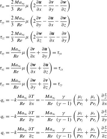 \begin{align}{\tau _{xx}} & = \frac{2}{3}\frac{{M{a_\infty }}}{{Re}}\mu \left( {2\frac{{\partial \boldsymbol{u}}}{{\partial x}} - \frac{{\partial \boldsymbol{v}}}{{\partial y}} - \frac{{\partial \boldsymbol{w}}}{{\partial z}}} \right)\nonumber\\[4pt]{\tau _{yy}} & = \frac{2}{3}\frac{{M{a_\infty }}}{{Re}}\mu \left( {2\frac{{\partial \boldsymbol{v}}}{{\partial y}} - \frac{{\partial \boldsymbol{u}}}{{\partial x}} - \frac{{\partial \boldsymbol{w}}}{{\partial z}}} \right)\nonumber\\[4pt]{\tau _{zz}} & = \frac{2}{3}\frac{{M{a_\infty }}}{{Re}}\mu \left( {2\frac{{\partial \boldsymbol{w}}}{{\partial z}} - \frac{{\partial \boldsymbol{u}}}{{\partial x}} - \frac{{\partial \boldsymbol{v}}}{{\partial y}}} \right)\nonumber\\[4pt]{\tau _{xy}} & = \frac{{M{a_\infty }}}{{Re}}\mu \left( {\frac{{\partial \boldsymbol{v}}}{{\partial x}} + \frac{{\partial \boldsymbol{u}}}{{\partial y}}} \right) = {\tau _{yx}}\nonumber\\[4pt]{\tau _{xz}} & = \frac{{M{a_\infty }}}{{Re}}\mu \left( {\frac{{\partial \boldsymbol{w}}}{{\partial x}} + \frac{{\partial \boldsymbol{u}}}{{\partial z}}} \right) = {\tau _{zx}}\\[4pt]{\tau _{yz}} & = \frac{{M{a_\infty }}}{{Re}}\mu \left( {\frac{{\partial \boldsymbol{w}}}{{\partial y}} + \frac{{\partial \boldsymbol{v}}}{{\partial z}}} \right) = {\tau _{zy}}\nonumber\\[4pt]{q_x} & = - k\frac{{M{a_\infty }}}{{Re}}\frac{{\partial T}}{{\partial x}} = - \frac{{M{a_\infty }}}{{Re}}\frac{\gamma }{{(\gamma - 1)}}\left( {\frac{{{\mu _l}}}{{P{r_l}}} + \frac{{{\mu _t}}}{{P{r_t}}}} \right)\frac{{\partial \frac{p}{\rho }}}{{\partial x}}\nonumber\\[4pt]{q_y} & = - k\frac{{M{a_\infty }}}{{Re}}\frac{{\partial T}}{{\partial y}} = - \frac{{M{a_\infty }}}{{Re}}\frac{\gamma }{{(\gamma - 1)}}\left( {\frac{{{\mu _l}}}{{P{r_l}}} + \frac{{{\mu _t}}}{{P{r_t}}}} \right)\frac{{\partial \frac{p}{\rho }}}{{\partial y}}\nonumber\\[4pt]{q_z} & = - k\frac{{M{a_\infty }}}{{Re}}\frac{{\partial T}}{{\partial z}} = - \frac{{M{a_\infty }}}{{Re}}\frac{\gamma }{{(\gamma - 1)}}\left( {\frac{{{\mu _l}}}{{P{r_l}}} + \frac{{{\mu _t}}}{{P{r_t}}}} \right)\frac{{\partial \frac{p}{\rho }}}{{\partial z}}\nonumber\end{align}
The laminar viscosity coefficient ${\mu _l}$
is calculated by Sutherland’s formula (4).
${\mu _l}$
is calculated by Sutherland’s formula (4).
 \begin{align}\frac{{{\mu _l}}}{{{\mu _\infty }}} \approx {\left( {\frac{T}{{{T_\infty }}}} \right)^{\frac{3}{2}}}\left( {\frac{{{T_\infty } + {T_r}}}{{T + {T_r}}}} \right)\end{align}
Here, ${T_r}$
is the reference temperature.
${T_r}$
is the reference temperature. ${\mu _t}$
is the turbulent viscosity coefficient, calculated from the viscous model. The thermal conductivity coefficient
${\mu _t}$
is the turbulent viscosity coefficient, calculated from the viscous model. The thermal conductivity coefficient $k$
is given by
$k$
is given by
 \begin{align}k = {c_P}\left( {\frac{{{\mu _l}}}{{P{r_l}}} + \frac{{{\mu _t}}}{{P{r_t}}}} \right) = \frac{{\gamma R}}{{\left( {\gamma - 1} \right)}}\left( {\frac{{{\mu _l}}}{{P{r_l}}} + \frac{{{\mu _t}}}{{P{r_t}}}} \right)\end{align}
For air, the laminar Prandtl number $P{r_l}$
is 0.72, and the turbulent Prandtl number
$P{r_l}$
is 0.72, and the turbulent Prandtl number $P{r_t}$
is 0.9.
$P{r_t}$
is 0.9. ${c_P}$
and
${c_P}$
and $R$
are the mass heat capacity and gas constant, respectively. After dimensionless transformation, the ideal-gas equation becomes
$R$
are the mass heat capacity and gas constant, respectively. After dimensionless transformation, the ideal-gas equation becomes
 \begin{align}T = \gamma \frac{p}{\rho }\end{align}
The k- $\omega$
SST model is used for simulation. This model combines k-
$\omega$
SST model is used for simulation. This model combines k- $\omega$
and k-
$\omega$
and k- $\varepsilon$
in a weight average way. The k-
$\varepsilon$
in a weight average way. The k- $\varepsilon$
model has less dependence on far-field conditions, while the k-
$\varepsilon$
model has less dependence on far-field conditions, while the k- $\omega$
model has higher simulation accuracy near the wall [Reference Sun, Gerdroodbary, Abazari, Hosseini and Li29, Reference Liu, Gerdroodbary, Sheikholeslami, Moradi, Shafee and Li30]. The k-
$\omega$
model has higher simulation accuracy near the wall [Reference Sun, Gerdroodbary, Abazari, Hosseini and Li29, Reference Liu, Gerdroodbary, Sheikholeslami, Moradi, Shafee and Li30]. The k- $\omega$
SST model takes turbulent kinetic energy k and its specific dissipation rate
$\omega$
SST model takes turbulent kinetic energy k and its specific dissipation rate $\omega$
as solving variables, the latter of which is defined as
$\omega$
as solving variables, the latter of which is defined as
 \begin{align}\omega = \frac{\varepsilon }{{{\beta ^*}k}}\end{align}
The governing equation of the turbulence variables is described by
 \begin{align}\frac{{\partial \rho k}}{{\partial t}} + \frac{{\partial \rho vk}}{{\partial y}} = \tilde P - {\beta ^*}\rho \omega k + \frac{\partial }{{\partial y}}\left[ {\left( {{\mu _l} + {\sigma _k}{\mu _t}} \right)\frac{{\partial k}}{{\partial y}}} \right]\end{align}
 \begin{align}\frac{{\partial \rho \omega }}{{\partial t}} + \frac{{\partial \rho v\omega }}{{\partial y}} = \frac{\gamma }{{{\nu _t}}}P - \beta \rho {\omega ^2} + \frac{\partial }{{\partial y}}\left[ {\left( {{\mu _l} + {\sigma _\omega }{\mu _t}} \right)\frac{{\partial \omega }}{{\partial y}}} \right] + 2\left( {1 - {F_1}} \right)\frac{{\rho {\sigma _{\omega 2}}}}{\omega } \cdot \frac{{\partial k}}{{\partial y}} \cdot \frac{{\partial \omega }}{{\partial y}}\end{align}
In the above $\omega$
equation, the first three terms on the right are the generation term, dissipation term and diffusion term. The fourth term on the right is the cross-diffusion term.
$\omega$
equation, the first three terms on the right are the generation term, dissipation term and diffusion term. The fourth term on the right is the cross-diffusion term. $P$
,
$P$
, ${\tau _{xy}}$
and
${\tau _{xy}}$
and ${S_{xy}}$
are given by
${S_{xy}}$
are given by
 \begin{align}P = {\tau _{xy}}\frac{{\partial u}}{{\partial y}}\end{align}
 \begin{align}{\tau _{xy}} = {\mu _t}\left( {2{S_{xy}} - \frac{2}{3}\frac{{\partial w}}{{\partial z}}{\delta _{xy}}} \right) - \frac{2}{3}\rho k{\delta _{ij}}\end{align}
 \begin{align}{S_{xy}} = \frac{1}{2}\left( {\frac{{\partial u}}{{\partial y}} + \frac{{\partial v}}{{\partial x}}} \right)\end{align} $P$
in Equation (10) can be simplified to
$P$
in Equation (10) can be simplified to
 \begin{align}P = {\tau _{xy}}\frac{{\partial u}}{{\partial y}} = {\mu _t}\left[ {{{\left| S \right|}^2} - \frac{2}{3}{{\left( {\frac{{\partial w}}{{\partial z}}} \right)}^2}} \right] - \frac{2}{3}\rho k\frac{{\partial w}}{{\partial z}}\end{align}
In the k equation, $P$
needs to be restricted as
$P$
needs to be restricted as
 \begin{align}\tilde P = \min\! \left( {P,20{\beta ^*}\rho \omega k} \right)\end{align}
The turbulent viscosity coefficient is calculated according to Equation (14).
 \begin{align}{\mu _t} = \frac{{\rho {a_1}k}}{{\max \left( {{a_1}\omega ,\Omega {F_2}} \right)}}\end{align}
 \begin{align}{F_2} = \tanh \arg _2^2\end{align}
 \begin{align}{\arg _2} = \max \left( {2\frac{{\sqrt k }}{{{\beta ^*}\omega d}},\frac{{500\nu }}{{{d^2}\omega }}} \right)\end{align}
Here, $\varepsilon$
is the dissipation rate of the turbulent kinetic energy,
$\varepsilon$
is the dissipation rate of the turbulent kinetic energy, ${\nu _t}$
is the turbulent kinematic viscosity,
${\nu _t}$
is the turbulent kinematic viscosity, $\nu $
is the molecular kinematic viscosity,
$\nu $
is the molecular kinematic viscosity, ${\tau _{xy}}$
is the viscous shear stress,
${\tau _{xy}}$
is the viscous shear stress, $\Omega $
is the rotation amplitude and
$\Omega $
is the rotation amplitude and $d$
is the distance from the grid point to the nearest solid wall.
$d$
is the distance from the grid point to the nearest solid wall. ${\beta ^*}$
,
${\beta ^*}$
, $\beta $
,
$\beta $
, ${\sigma _k}$
,
${\sigma _k}$
, ${\sigma _\omega }$
,
${\sigma _\omega }$
, ${\sigma _{\omega 2}}$
and
${\sigma _{\omega 2}}$
and ${a_1}$
are closed constants. The above equations were solved using the commercial CFD software Fluent.
${a_1}$
are closed constants. The above equations were solved using the commercial CFD software Fluent.
2.2 Validation
All of the simulations in this work are 2D and based on the model and boundary conditions as illustrated in Fig. 2. The duct has a length $L$
of 700mm and a height
$L$
of 700mm and a height $H$
of 36mm.
$H$
of 36mm. ${p_b}$
is the outlet pressure,
${p_b}$
is the outlet pressure, ${p_a}$
is the inlet pressure, and
${p_a}$
is the inlet pressure, and ${t_0}$
is the backpressure duration. The Mach number at the isolator inlet is 1.61, and the total pressure is 206,000Pa. A pulse backpressure is imposed at the isolator exit by a prescribed pressure ratio
${t_0}$
is the backpressure duration. The Mach number at the isolator inlet is 1.61, and the total pressure is 206,000Pa. A pulse backpressure is imposed at the isolator exit by a prescribed pressure ratio ${p_b}\!\left( t \right)/{p_a}$
and duration
${p_b}\!\left( t \right)/{p_a}$
and duration ${t_0}$
. The duct walls are considered adiabatic and subject to a no-slip boundary condition, upon which the transient simulation of pulse backpressure cases was carried out. The inlet and outlet boundary conditions of the steady case are, respectively, pressure inlet and pressure outlet, which are the same as the pressure in literature [Reference Carroll and Dutton31]. A synthetic turbulence-generation method [Reference Kim, Xie and Castro32, Reference Kim33] is utilised at the inflow plane to generate the boundary turbulence of the steady case. It first generates a 2D slice
${t_0}$
. The duct walls are considered adiabatic and subject to a no-slip boundary condition, upon which the transient simulation of pulse backpressure cases was carried out. The inlet and outlet boundary conditions of the steady case are, respectively, pressure inlet and pressure outlet, which are the same as the pressure in literature [Reference Carroll and Dutton31]. A synthetic turbulence-generation method [Reference Kim, Xie and Castro32, Reference Kim33] is utilised at the inflow plane to generate the boundary turbulence of the steady case. It first generates a 2D slice $r\left( {t,j,k} \right)$
of random numbers with a mean of zero and a variance of one on the inlet surface. By manipulating the correlation in the y-direction (Equation (19)) and the z-direction (Equation (20)), the correlation in the x-direction is implemented (Equation (21)). The final inflow velocity is obtained by Equation (22).
$r\left( {t,j,k} \right)$
of random numbers with a mean of zero and a variance of one on the inlet surface. By manipulating the correlation in the y-direction (Equation (19)) and the z-direction (Equation (20)), the correlation in the x-direction is implemented (Equation (21)). The final inflow velocity is obtained by Equation (22). $\phi (t,j,k)$
and
$\phi (t,j,k)$
and $\psi (t,j,k)$
are intermediate variables.In the transient case, the inlet boundary condition is set as pressure inlet. The pressure distribution is derived from converting the velocity distribution obtained through the previously mentioned method. However, during the trial calculation of the transient case, a reverse flow was observed at the outlet upon applying the pulse backpressure. Consequently, the pressure outlet cannot serve as the outlet condition. Unlike the pressure outlet, the pressure inlet is not restricted by forward flow conditions. Hence, the pressure inlet is chosen as the outlet boundary condition for the transient case, with pulse backpressure control facilitated through a user-defined function (UDF).
$\psi (t,j,k)$
are intermediate variables.In the transient case, the inlet boundary condition is set as pressure inlet. The pressure distribution is derived from converting the velocity distribution obtained through the previously mentioned method. However, during the trial calculation of the transient case, a reverse flow was observed at the outlet upon applying the pulse backpressure. Consequently, the pressure outlet cannot serve as the outlet condition. Unlike the pressure outlet, the pressure inlet is not restricted by forward flow conditions. Hence, the pressure inlet is chosen as the outlet boundary condition for the transient case, with pulse backpressure control facilitated through a user-defined function (UDF).
Figure 2. Outline of the general flow arrangement.
 \begin{align}\phi (t,j + 1,k) = \phi (t,j,k)\exp \left( { - \frac{1}{{{n_y}}}} \right) + r\left( {t,j,k} \right){\left[ {1 - \exp \left( { - \frac{2}{{{n_y}}}} \right)} \right]^{0.5}}\end{align}
 \begin{align}\psi (t,j,k + 1) = \psi (t,j,k)\exp \left( { - \frac{1}{{{n_z}}}} \right) + \phi \left( {t,j,k} \right){\left[ {1 - \exp \left( { - \frac{2}{{{n_z}}}} \right)} \right]^{0.5}}\end{align}
 \begin{align}{u^*}(t + \Delta t,j,k) = {u^*}(t,j,k)\exp \left( { - \frac{1}{{{n_t}}}} \right) + \psi \left( {t,j,k} \right){\left[ {1 - \exp \left( { - \frac{2}{{{n_t}}}} \right)} \right]^{0.5}}\end{align}
 \begin{align}{u_i} = {U_i} + {a_{ij}}u_j^*\end{align}
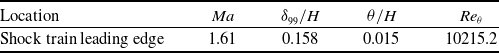
The key boundary layer properties, such as turbulence intensity, skin friction, and correlation lengths, converge after an axial distance of $6H$
from the inlet. This is the region where the shock wave caused by backpressure disturbance can reach its maximum position upstream, and full details of the flow parameters just upstream of the shock train are presented in Table 1.
$6H$
from the inlet. This is the region where the shock wave caused by backpressure disturbance can reach its maximum position upstream, and full details of the flow parameters just upstream of the shock train are presented in Table 1.
Table 1. Summary of flow parameters at the shock train leading edge
To verify the rationality of the numerical simulation method, the simulation of the rectangular section isolator experiment of Carroll and Dutton [Reference Carroll and Dutton31] was conducted using the above method. The fourth condition in Mach 1.6 cases is selected, where the thickness of the inlet boundary layer is ${\delta _a} = 5.4{\kern 1pt} {\kern 1pt} {\kern 1pt} mm$
, and the outlet to inlet pressure ratio
${\delta _a} = 5.4{\kern 1pt} {\kern 1pt} {\kern 1pt} mm$
, and the outlet to inlet pressure ratio ${p_b}/{p_a} = 2.41$
. Figure 3 displays the Schlieren image obtained by experiment (a) and the simulation method (b) above. The simulation results capture the shape and spacing of the first three shock waves well, which is very close to the experiment result. The black curve and red scatter points in Fig. 4 represent the dimensionless wall static pressure distribution obtained by simulation and experiment in Ref. (Reference Carroll and Dutton31), respectively. The magnitude and distribution of the wall static pressure obtained by simulation are very close to the experiment values. Thus, it can be considered that the above numerical simulation method can produce reliable flow field results.
${p_b}/{p_a} = 2.41$
. Figure 3 displays the Schlieren image obtained by experiment (a) and the simulation method (b) above. The simulation results capture the shape and spacing of the first three shock waves well, which is very close to the experiment result. The black curve and red scatter points in Fig. 4 represent the dimensionless wall static pressure distribution obtained by simulation and experiment in Ref. (Reference Carroll and Dutton31), respectively. The magnitude and distribution of the wall static pressure obtained by simulation are very close to the experiment values. Thus, it can be considered that the above numerical simulation method can produce reliable flow field results.
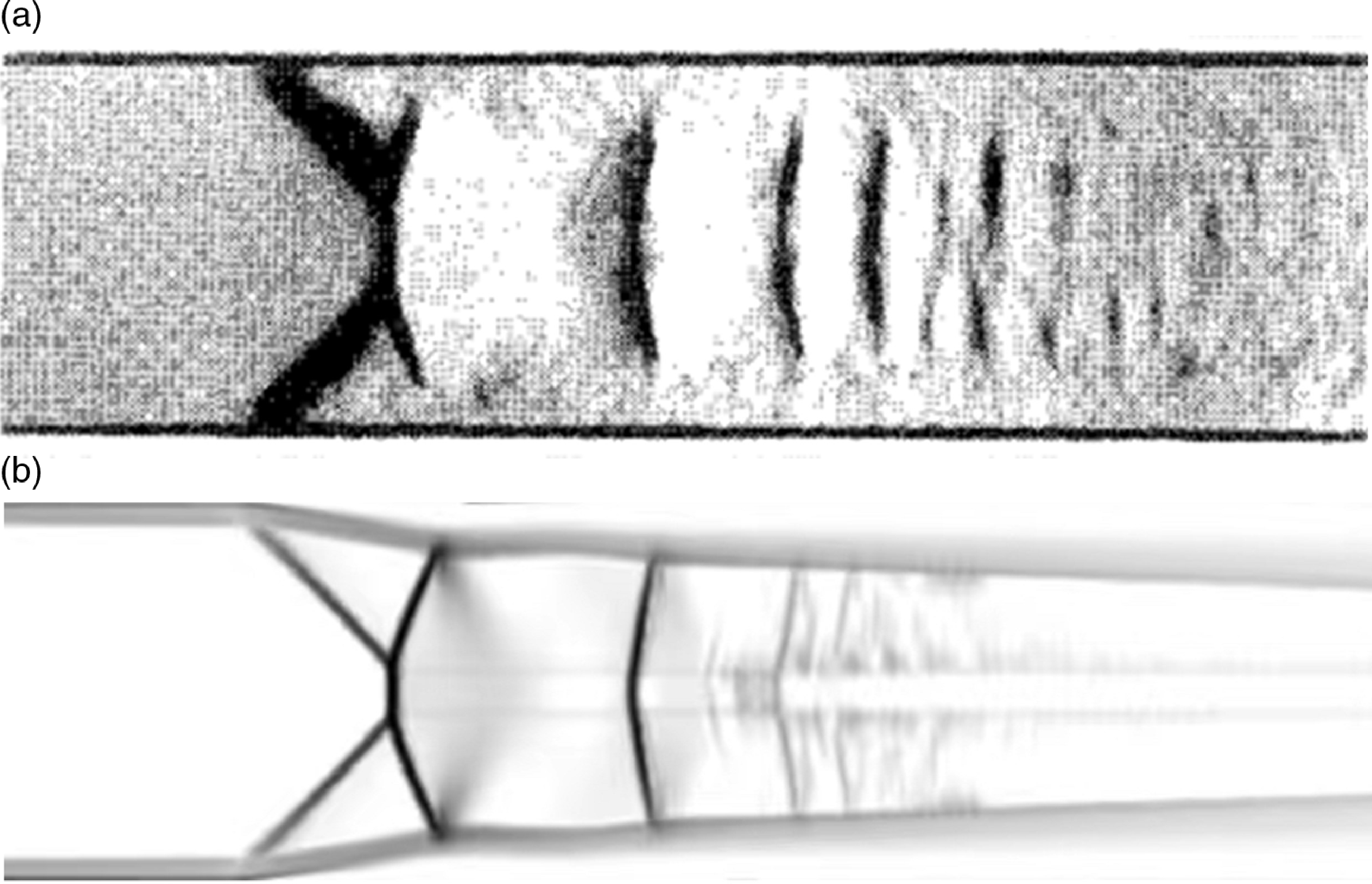
Figure 3. Schlieren image obtained by experiment (a) and simulation (b).
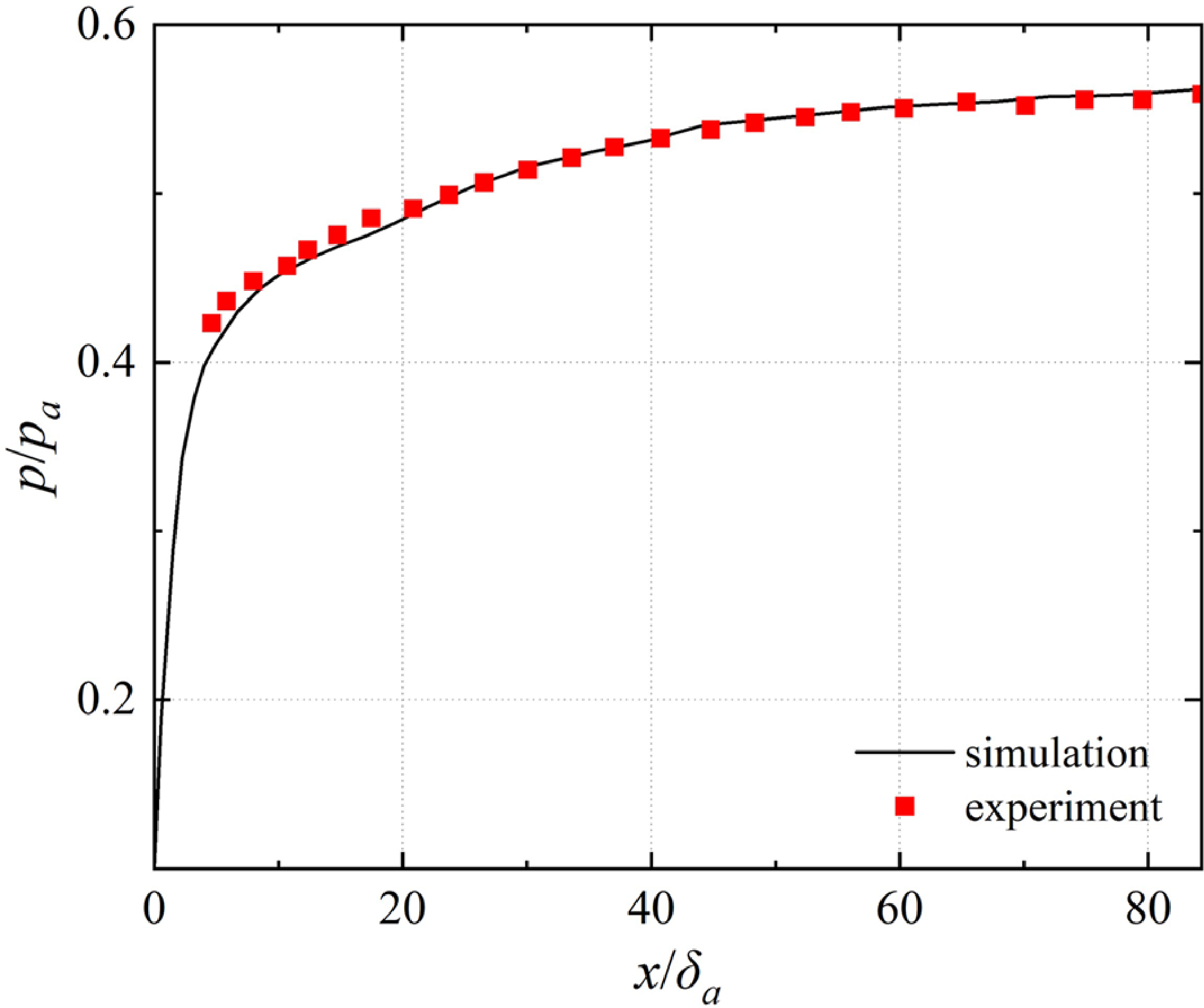
Figure 4. Wall static pressure distribution obtained by experiment and numerical simulation.
2.3 Grid refinement study
The calculation domain is a rectangular region with a length of 700mm and a height of 35mm, filled with structural grids. A grid refinement study was carried out over three grid resolutions to investigate the sensitivity of the shock train flow properties. The number of cells in Grid 1, Grid 2, and Grid 3 was 3 × 10⁵, 2 × 10⁵, and 0.8 × 10⁵, respectively. In the present study, the grid closer to the wall is clustered in the direction perpendicular to the flow direction to maintain a wall Y+ value of about 0.93.
Figure 5(a) is the grid with 200,000 cells within the computational domain, and Fig. 5(b) is its enlarged view near the inlet. The grid distribution in the x-direction is uniform, with a grid size of about 0.4mm. In the y-direction, densification was performed near the wall, with the Y+ of the first layer being about 0.93 and the maximum grid size appearing on the centreline at 0.4mm. The maximum grid size in the entire fluid is 0.3mm, and all grids are orthogonal.
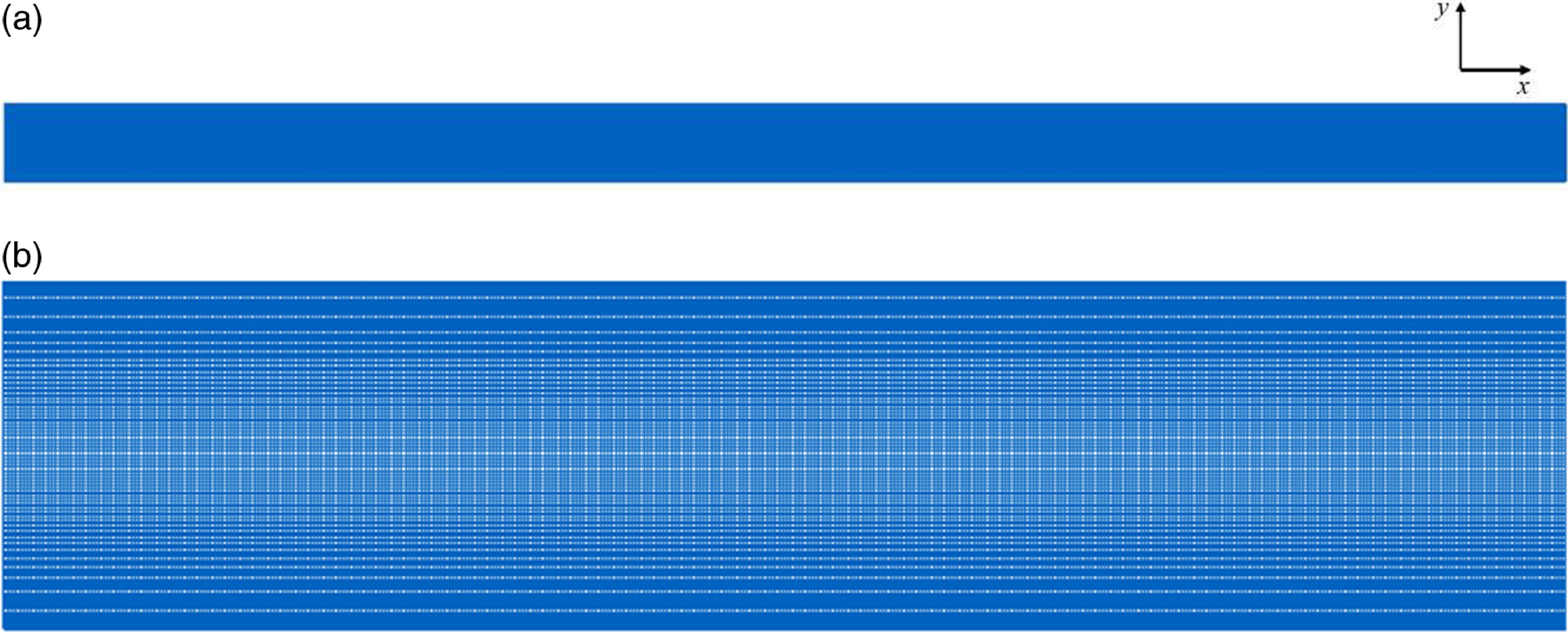
Figure 5. Grid with 200,000 cells within the computational domain (a) and the enlarged view near the inlet (b).
The results of the grid study are presented in Fig. 6, which compares the streamwise and wall distributions of static pressure at a certain time after the shock train formation. The shock positions can be recognised clearly in Fig. 6(a) as the sharp peaks in pressure. In Fig. 6(b), the wall static pressure along the path shows a slow upward trend followed by a gradual decrease. The rise of the leading edge is attributed to subsonic turbulence in the boundary layer region. At the same time, the subsequent decline is a consequence of the reduction of pressure at the outlet. It is evident from these results that the coarser grid resolution leads to a downstream shift in the shock positions, and the numerical dissipation caused by grid dissipation is also greater, although the overall structure of the shock train remains intact.
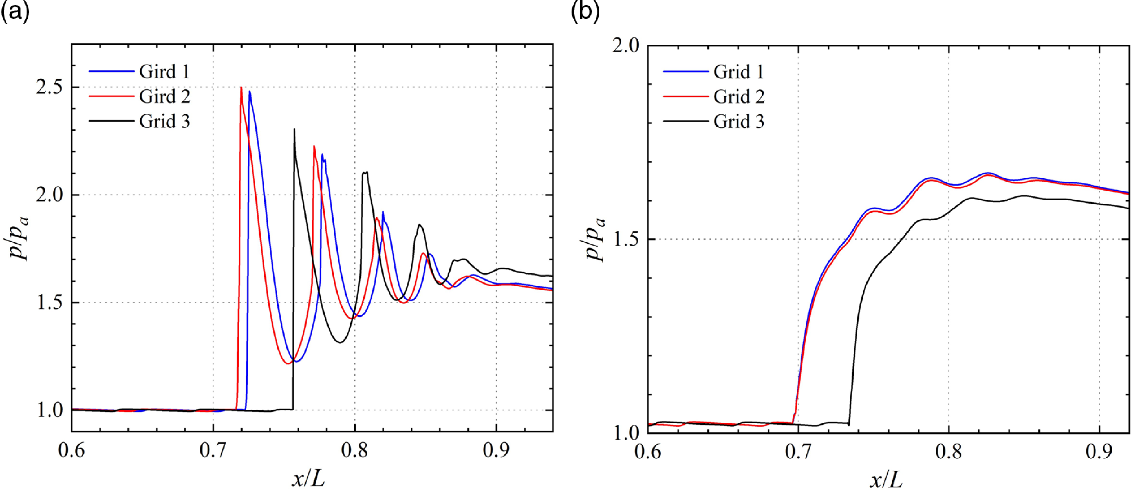
Figure 6. Comparison of pressure distributions streamwise (a) and nearwall (b) for the different grid resolutions.
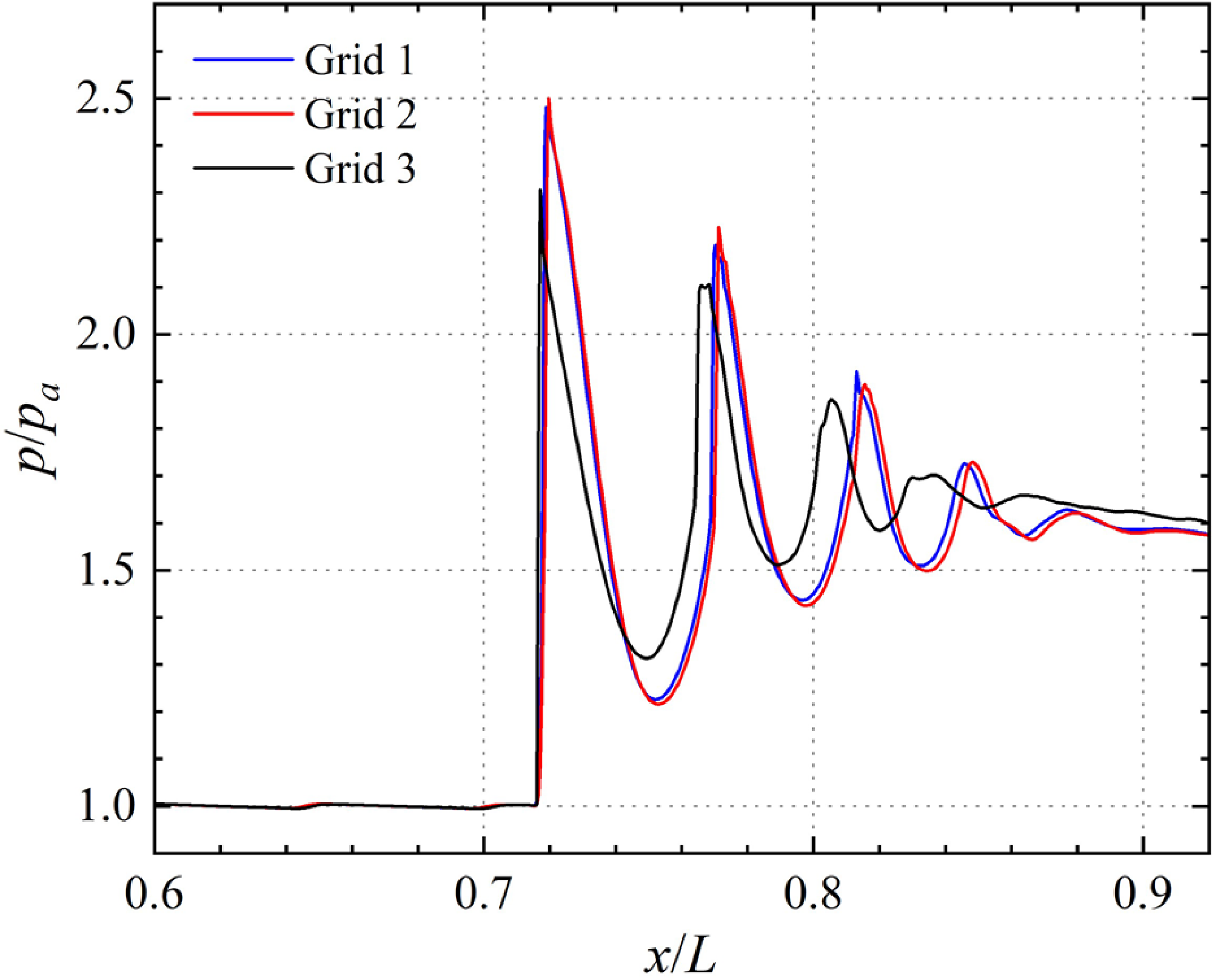
Figure 7. Plots of centreline pressure, normalised by the leading shock position.
The first rising position of the three curves in Fig. 6(a) differs, indicating that the first shock wave appears at different locations. This discrepancy limits the intuitive observation of the shock string length that we aim to investigate. To facilitate a more direct comparison and identification of the differences between the three curves, we plot the centreline pressure again in Fig. 7 but adjust the red and blue curves horizontally to match the location of the first shock. The results of Grid 2 and Grid 3 are well-matched throughout the shock train, including the strength and spacing of the shock waves. However, the result of Grid 1 differs significantly from those of the other two grids, with smaller shock intensity and spacing. As the shock spacing can be identified during the dynamic response, and the results of Grid 2 and Grid 3 are nearly identical, we conclude that the dynamic behaviour of the shock train can be accurately captured by either Grid 2 or Grid 3.
The time evolution of the leading shock and the second shock location for three grid resolutions is shown in Fig. 8. The difference between Grid 2 and Grid 3 is minor, while the difference between Grid 1 and the other two is substantial. Furthermore, the shock wave spacing in Grid 1 is smaller. Although the position that the leading shock wave can reach the upstream end in three results is different (Gird 1 and Gird 2 settle further upstream, as in Fig. 5), the moving trajectory and dynamic response time are consistent. The results for the three grid resolutions are similar regarding the lag of dynamic response to changing backpressure. Considering the accuracy of shock wave structure and length and the calculation cost, all subsequent transient numerical simulation is based on Grid 2.
Table 2. Backpressure peak, duration and dimensionless maximum backpropagation distance to different cases
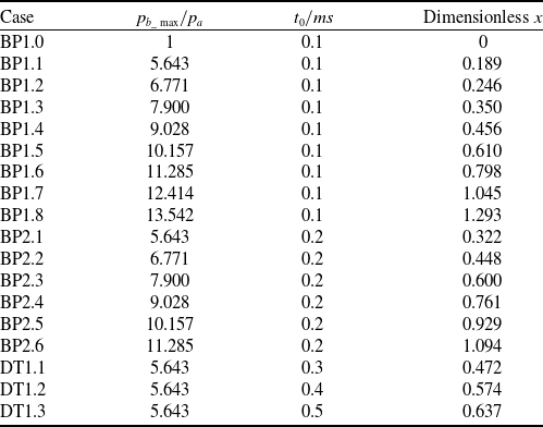
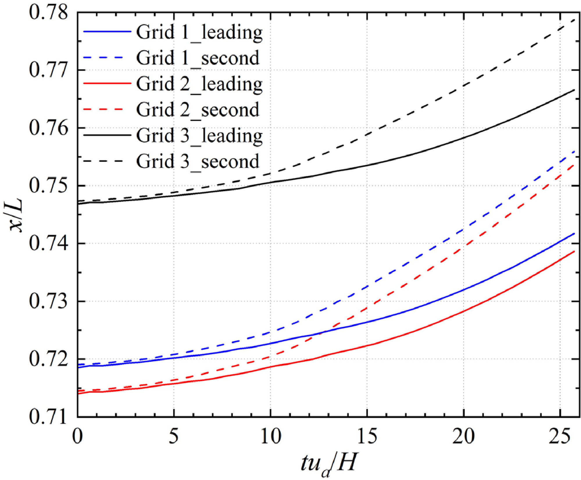
Figure 8. Time evolution of the leading and second shock position after the disturbance reaches the upstream end.
3.0 Basic analysis
3.1 Time history analysis
In this section, we will study the response of the shock wave system to the amplitude and duration of pulse backpressure. Here, the time-varying backpressure takes the form
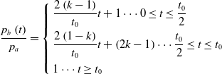 \begin{align}\dfrac{{{p_b}\left( t \right)}}{{{p_a}}} = \left\{ \begin{array}{l}\dfrac{{2\left( {k - 1} \right)}}{{{t_0}}}t + 1 \cdots 0 \le t \le \dfrac{{{t_0}}}{2}\\[9pt]\dfrac{{2\left( {1 - k} \right)}}{{{t_0}}}t + \left( {2k - 1} \right) \cdots \dfrac{{{t_0}}}{2} \le t \le {t_0}\\[9pt]1 \cdots t \geq {t_0}\end{array} \right.\end{align}
where ${p_b}\!\left( t \right)$
is backpressure,
${p_b}\!\left( t \right)$
is backpressure, ${t_0}$
is the duration of pulse backpressure, and
${t_0}$
is the duration of pulse backpressure, and $k$
is the ratio of peak pulse backpressure
$k$
is the ratio of peak pulse backpressure ${p_{b\_\max }}$
to the outlet pressure when the flow is stable before the disturbance is applied. The pulse backpressure begins at time
${p_{b\_\max }}$
to the outlet pressure when the flow is stable before the disturbance is applied. The pulse backpressure begins at time $t = 0$
when the flow is assumed to be at a steady state. Dimensionless pulse backpressure peak and duration of different cases are given in Table 2. BP1.0–BP1.8 and BP2.1–BP2.6 all changed the peak of pulse backpressure. The difference between the two groups is that the duration of backpressure is 0.1 and 0.2ms respectively. The backpressure peak of DT1.1–DT1.3 is the same, the only difference is duration.
$t = 0$
when the flow is assumed to be at a steady state. Dimensionless pulse backpressure peak and duration of different cases are given in Table 2. BP1.0–BP1.8 and BP2.1–BP2.6 all changed the peak of pulse backpressure. The difference between the two groups is that the duration of backpressure is 0.1 and 0.2ms respectively. The backpressure peak of DT1.1–DT1.3 is the same, the only difference is duration.
The value of ${p_{b\_max}}$
and
${p_{b\_max}}$
and ${t_0}$
is obtained from the detonation combustion case in the coupling model of the inlet, isolator, and combustor, which operates at Mach 2.5 and an altitude of 11km. The pressure distribution in the PDR isolator when the backpropagating shock wave reaches the upstream end is presented in Fig. 9. Hydrogen is chosen as the fuel, and the incoming air serves as the oxidant. Once the inlet establishes a stable wave system, the hydrogen mass source is introduced to the inlet of the combustor. When the hydrogen is about to fill the combustor, a high temperature and pressure zone is set at the front of the combustor to initiate combustion, thereby ensuring that the values of
${t_0}$
is obtained from the detonation combustion case in the coupling model of the inlet, isolator, and combustor, which operates at Mach 2.5 and an altitude of 11km. The pressure distribution in the PDR isolator when the backpropagating shock wave reaches the upstream end is presented in Fig. 9. Hydrogen is chosen as the fuel, and the incoming air serves as the oxidant. Once the inlet establishes a stable wave system, the hydrogen mass source is introduced to the inlet of the combustor. When the hydrogen is about to fill the combustor, a high temperature and pressure zone is set at the front of the combustor to initiate combustion, thereby ensuring that the values of ${p_{b\_max}}$
and
${p_{b\_max}}$
and ${t_0}$
are consistent with the parameters observed in actual detonation combustion vehicles. Additional information and validations of this case can be found in Chapters 1, 2 and 3 of Ref. (Reference Ma, Li, Zhang and Fan34).
${t_0}$
are consistent with the parameters observed in actual detonation combustion vehicles. Additional information and validations of this case can be found in Chapters 1, 2 and 3 of Ref. (Reference Ma, Li, Zhang and Fan34).
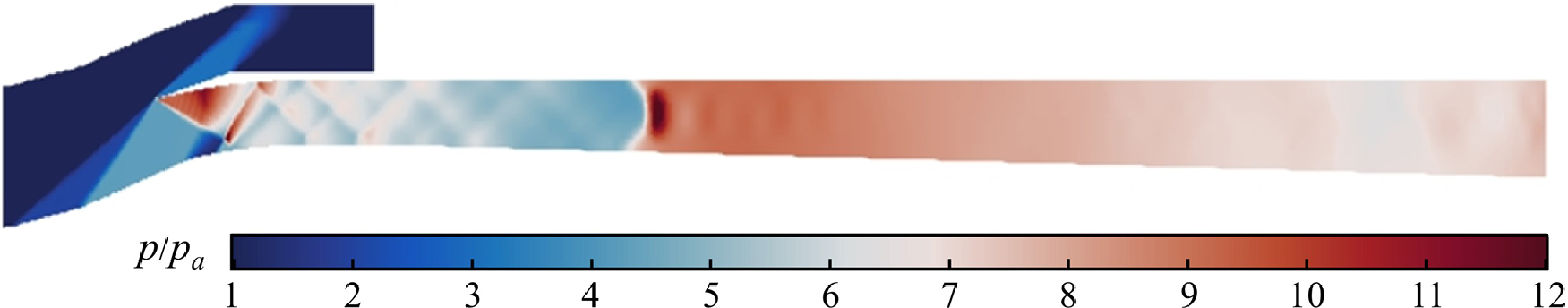
Figure 9. Pressure distribution in PDR isolator.
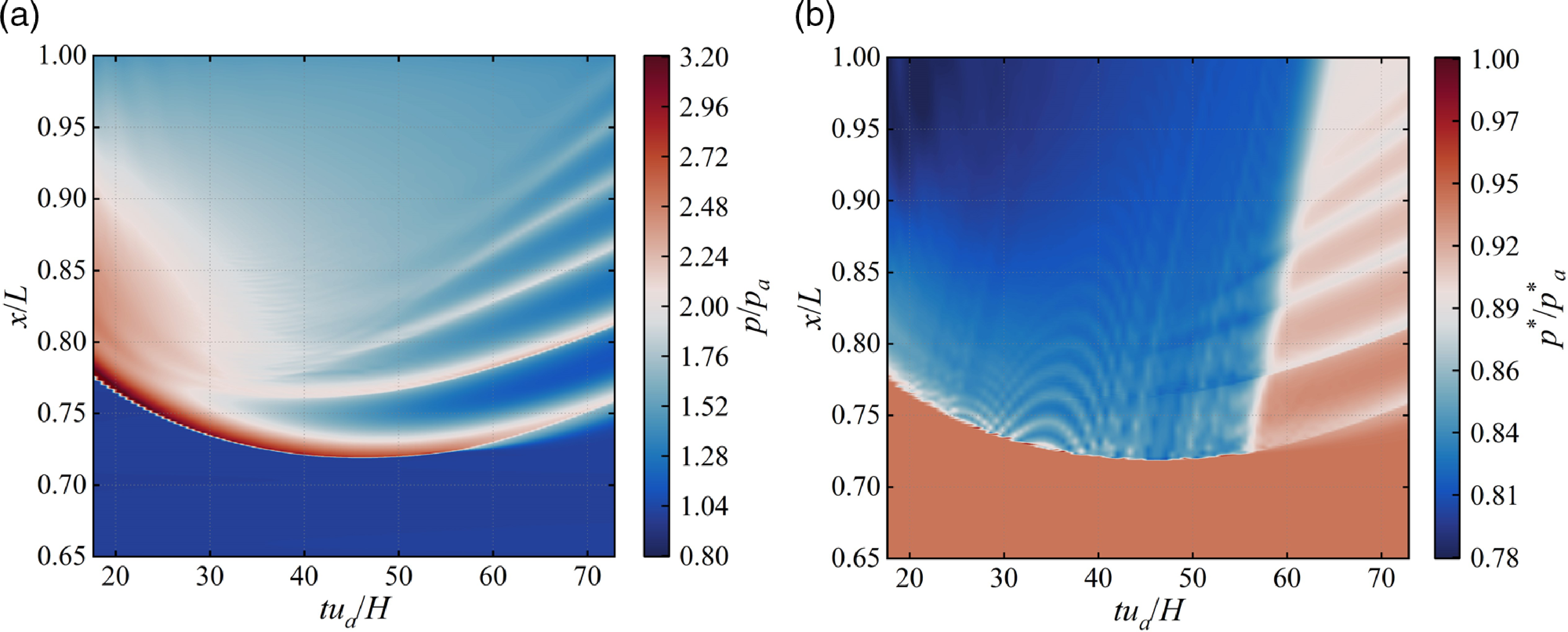
Figure 10. Time evolution of the pressure (a) and total pressure recovery (b) along the shock train centreline of BP1.6.
Figure 10(a) shows the time evolution of pressure distribution along the centreline of BP1.6. The abscissa represents the time, dimensionless by the inlet velocity ${u_a}$
and height
${u_a}$
and height $H$
. The ordinate represents the pipe position along the flow direction, dimensionless by the pipe length
$H$
. The ordinate represents the pipe position along the flow direction, dimensionless by the pipe length $L$
. The dimensionless time at which the forcing backpressure peak occurs is 0.64. In the contrast, the dimensionless time when the backpropagating shock wave reaches the upstream end is 47.835, which is very much behind the forcing backpressure peak. It indicates a pronounced forcing-response lag, which means that the boundary conditions applied at the outlet cannot quickly affect the upstream flow. The pressure disturbance propagates upstream with time in the form of a normal shock wave, with the typical characteristic of pressure rise after the shock wave. As time increases, the normal shock degenerates into a
$L$
. The dimensionless time at which the forcing backpressure peak occurs is 0.64. In the contrast, the dimensionless time when the backpropagating shock wave reaches the upstream end is 47.835, which is very much behind the forcing backpressure peak. It indicates a pronounced forcing-response lag, which means that the boundary conditions applied at the outlet cannot quickly affect the upstream flow. The pressure disturbance propagates upstream with time in the form of a normal shock wave, with the typical characteristic of pressure rise after the shock wave. As time increases, the normal shock degenerates into a $\lambda $
shock and a compression wave behind it, owing to the effects of viscous dissipation in the boundary layer, forming a multi-stage shock train. The intensity of the first shock keeps weakening from the outset, and the influence range of the high-pressure zone and shock train behind it expands over time. Notably, the shock train formation occurs before reaching the furthest point and becomes more distinct with time. Figure 10(b) illustrates the time evolution of the total pressure recovery distribution along the centreline of BP1.6. The total pressure recovery
$\lambda $
shock and a compression wave behind it, owing to the effects of viscous dissipation in the boundary layer, forming a multi-stage shock train. The intensity of the first shock keeps weakening from the outset, and the influence range of the high-pressure zone and shock train behind it expands over time. Notably, the shock train formation occurs before reaching the furthest point and becomes more distinct with time. Figure 10(b) illustrates the time evolution of the total pressure recovery distribution along the centreline of BP1.6. The total pressure recovery ${p^*}/{p_a}$
is the ratio of local total pressure to the total pressure at the inlet. At any time, the total pressure after the leading shock on the centreline decreases along the flow direction. However, the total pressure recovery through the shock train is significantly higher than that after a normal shock in the early stage. Furthermore, the total pressure at the outlet also increases with time.
${p^*}/{p_a}$
is the ratio of local total pressure to the total pressure at the inlet. At any time, the total pressure after the leading shock on the centreline decreases along the flow direction. However, the total pressure recovery through the shock train is significantly higher than that after a normal shock in the early stage. Furthermore, the total pressure at the outlet also increases with time.
3.2 Difference between pulse backpressure case and stable backpressure case
Figure 11 compares the maximum backpropagation distance obtained through transient numerical simulation (purple scatter points) and the steady shock train length determined using the Waltrup formula by bringing the peak backpressure (green scatter points). The results show that the maximum backpropagation distance is considerably smaller than the steady shock train length. Applying the Waltrup formula to obtain the maximum backpropagation distance for pulse backpressure is inappropriate because this formula is based on a fitting law derived from steady-state experiments. When the backpressure changes significantly, this law is no longer applicable. Nonetheless, the data distribution indicates a possible quadratic relationship between $x$
and
$x$
and ${p_f}/{p_a} - 1$
. As a result, it may be possible to utilise the same quadratic function relationship in Ref. (Reference Waltrup and Billing16) to fit the data and obtain a suitable fitting law for pulse backpressure.
${p_f}/{p_a} - 1$
. As a result, it may be possible to utilise the same quadratic function relationship in Ref. (Reference Waltrup and Billing16) to fit the data and obtain a suitable fitting law for pulse backpressure.
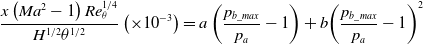
 \begin{align}{x_{stable}} = \frac{{x\left( {Ma_a^2 - 1} \right)Re_\theta ^{1/4}}}{{{D^{1/2}}{\theta ^{1/2}}}} = 50\left( {\frac{{{p_{b\_stable}}}}{{{p_a}}} - 1} \right) + 170{\left( {\frac{{{p_{b\_stable}}}}{{{p_a}}} - 1} \right)^2}\end{align}
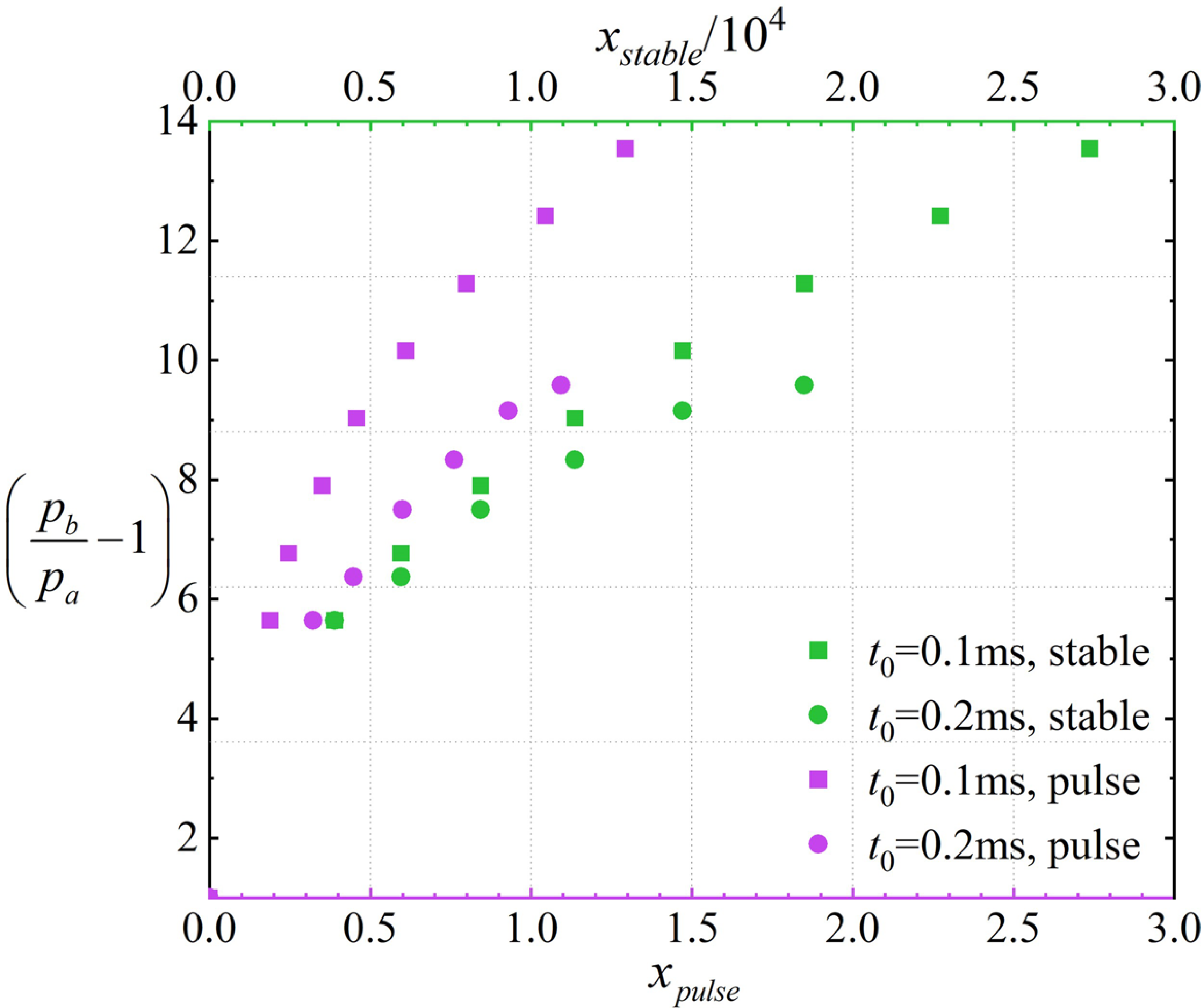
Figure 11. Maximum backpropagation distance from the simulation of BP1.0–2.6 and steady shock train length.
Figure 12 depicts the pressure distribution on the centreline and the Mach number distribution at five distinct moments. The first two moments illustrate the propagation of a pressure disturbance upstream, which exists in the form of a normal shock. The dimensionless pressure after the normal shock wave weakens from 4 to 3.5, indicating that the intensity of the pressure disturbance gradually weakens as it propagates upstream, and the stagnation effect on the flow gradually weakens.
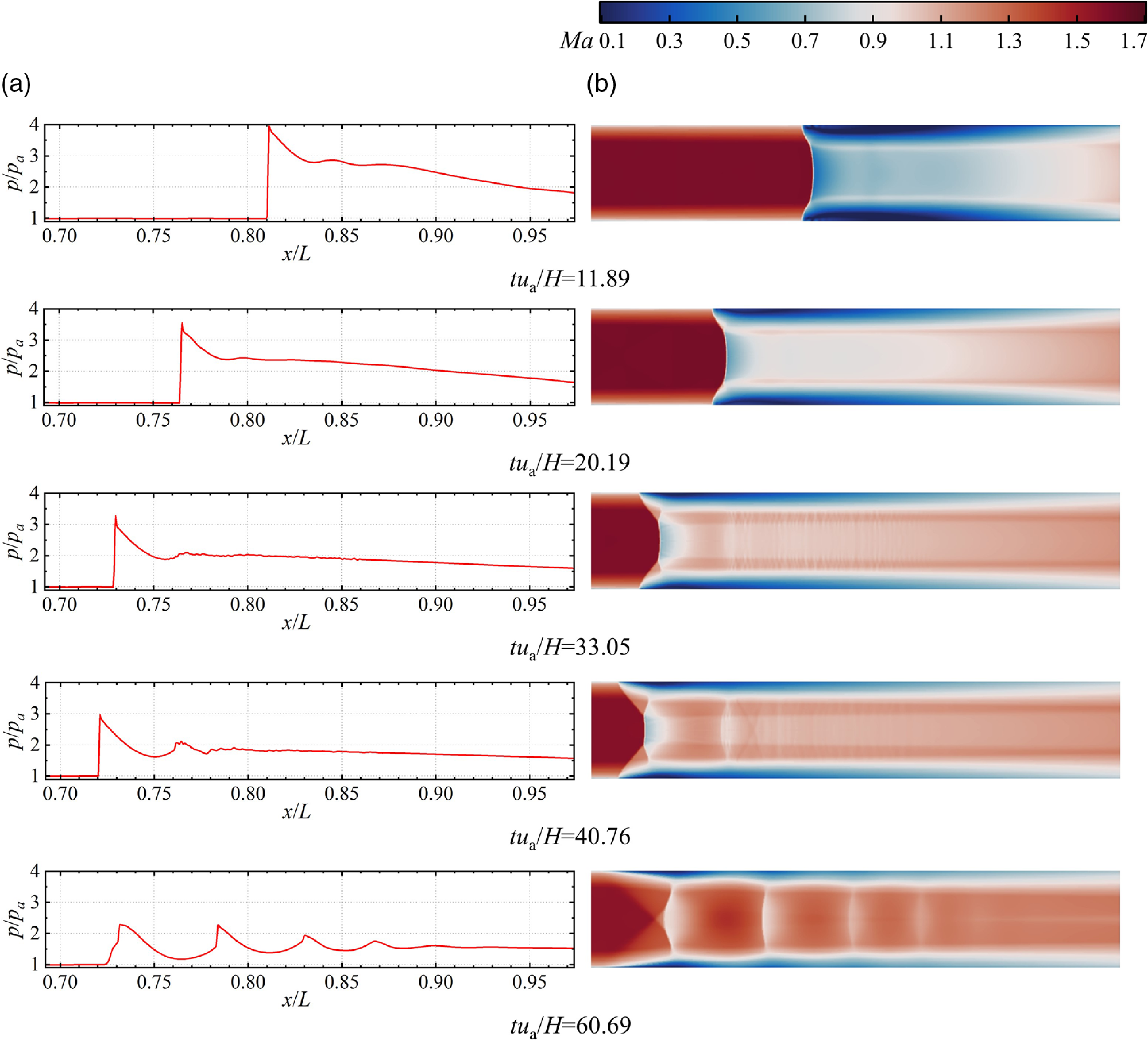
Figure 12. Pressure distribution in centreline (a) and Mach number distribution (b) of BP1.6.
As the leading shock approaches the upstream end, a series of weak compressional waves with tiny spacing form in the stagnation zone behind it. This compressional wave also exerts a certain stagnation effect. Once the pressure disturbance reaches the upstream end, the weak compression wave behind the leading shock gradually transforms into a recognisable shock train. Throughout the downstream movement of the leading shock, the shock train remains distinctly visible, and the spacing between shocks remains almost unchanged over time. In addition, comparing the Mach number distribution of five typical moments, it can be found that the Mach number of the mainstream at the outlet of the isolator increases from beginning to end, but the boundary layer thickness at the outlet remains almost unchanged, which means that the average Mach number at the outlet rises with time.
4.0 Maximum backpropagation distance analysis
4.1 Relationship between maximum backpropagation distance and backpressure peak
This section studies the relationship between maximum backpropagation distance and pressure peak. The maximum backpropagation distance $x$
refers to the farthest distance on the centreline that the leading edge of the pressure disturbance can travel after the application of pulse backpressure, which is in dimensionless form as shown by the abscissa in Fig. 13. Computational fluid dynamics results are used to obtain the Mach number of the mainstream in the undisturbed region upstream of the shock train, as well as the boundary-layer thickness
$x$
refers to the farthest distance on the centreline that the leading edge of the pressure disturbance can travel after the application of pulse backpressure, which is in dimensionless form as shown by the abscissa in Fig. 13. Computational fluid dynamics results are used to obtain the Mach number of the mainstream in the undisturbed region upstream of the shock train, as well as the boundary-layer thickness $\delta $
required to boundary-layer momentum thickness calculation, and the density and viscosity distribution that is needed in the calculation of
$\delta $
required to boundary-layer momentum thickness calculation, and the density and viscosity distribution that is needed in the calculation of $R{e_\theta }$
.
$R{e_\theta }$
.
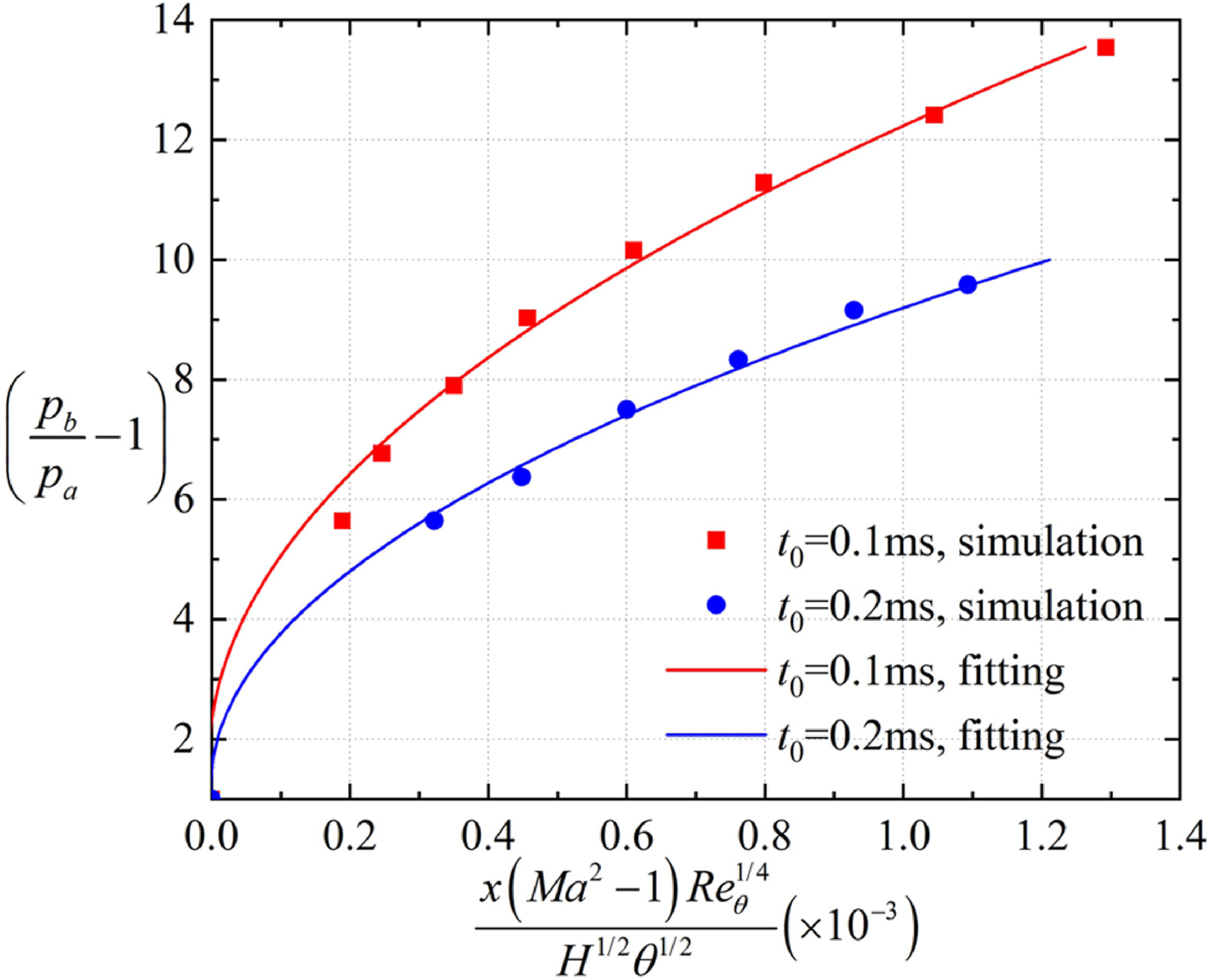
Figure 13. Dimensionless backpressure peak and maximum backpropagation distance of BP1.0–BP2.6.
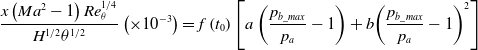
The red and blue scatter points in Fig. 13 represent the dimensionless backpressure peak and maximum backpropagation distance for BP1.0–BP1.8 and BP2.1–BP2.6, which seems to meet the quadratic function. The red scatters are fitted to a quadratic function, as described in Ref. (Reference Waltrup and Billing16), resulting in the red line. The fitting formula is described by
 \begin{align}\frac{{x\left( {M{a^2} - 1} \right)Re_\theta ^{1/4}}}{{{H^{1/2}}{\theta ^{1/2}}}}\left( { \times {{10}^{ - 3}}} \right) = a\left( {\frac{{{p_{b\_max}}}}{{{p_a}}} - 1} \right) + b{\left( {\frac{{{p_{b\_max}}}}{{{p_a}}} - 1} \right)^2}\end{align}
Although the red points appear to conform to the quadratic relationship, determining the parameters $a$
and
$a$
and $b$
here is not meaningful because the maximum backpropagation distance depends not only on the backpressure peak but also on the duration. Formula (25) fails to capture the relationship between the maximum backpropagation distance and backpressure duration. For instance, as the backpressure duration increases from 0.1ms (red scatter points) to 0.2ms (blue scatter points), parameters
$b$
here is not meaningful because the maximum backpropagation distance depends not only on the backpressure peak but also on the duration. Formula (25) fails to capture the relationship between the maximum backpropagation distance and backpressure duration. For instance, as the backpressure duration increases from 0.1ms (red scatter points) to 0.2ms (blue scatter points), parameters $a$
and
$a$
and $b$
will change as well. Therefore, the relationship may be expressed as follows.
$b$
will change as well. Therefore, the relationship may be expressed as follows.
 \begin{align}\frac{{x\left( {M{a^2} - 1} \right)Re_\theta ^{1/4}}}{{{H^{1/2}}{\theta ^{1/2}}}}\left( { \times {{10}^{ - 3}}} \right) = f\left( {{t_0}} \right)\left[ {a\left( {\frac{{{p_{b\_max}}}}{{{p_a}}} - 1} \right) + b{{\left( {\frac{{{p_{b\_max}}}}{{{p_a}}} - 1} \right)}^2}} \right]\end{align}
That is, $x$
is proportional to
$x$
is proportional to $a\left( {{p_{b\_max}}/{p_a} - 1} \right) + b{\left( {{p_{b\_max}}/{p_a} - 1} \right)^2}$
, but the determination requires specifying the backpressure duration
$a\left( {{p_{b\_max}}/{p_a} - 1} \right) + b{\left( {{p_{b\_max}}/{p_a} - 1} \right)^2}$
, but the determination requires specifying the backpressure duration ${t_0}$
. Notably,
${t_0}$
. Notably, $a$
and
$a$
and $b$
in formula (26) are different from those in formula (13). The former is obtained by surface fitting of variables
$b$
in formula (26) are different from those in formula (13). The former is obtained by surface fitting of variables $\left( {{p_{b\_max}}/{p_a} - 1} \right)$
and
$\left( {{p_{b\_max}}/{p_a} - 1} \right)$
and ${t_0}$
, which is the final result with reference significance. The latter is obtained by curve fitting of
${t_0}$
, which is the final result with reference significance. The latter is obtained by curve fitting of $\left( {{p_{b\_max}}/{p_a} - 1} \right)$
and only facilitates understanding the relationship between
$\left( {{p_{b\_max}}/{p_a} - 1} \right)$
and only facilitates understanding the relationship between $x$
and
$x$
and $\left( {{p_{b\_max}}/{p_a} - 1} \right)$
.
$\left( {{p_{b\_max}}/{p_a} - 1} \right)$
.
4.2 Relationship between maximum backpropagation distance and backpressure duration
Figure 14 presents scatter plots for the dimensionless maximum backpropagation distance and backpressure duration of BP1.1, BP2.1, and DT1.1–1.3. These values seem to align with a quadratic function. We employed the same method as in the previous section to fit the data and obtain the red curve. The fitting formula is provided below.
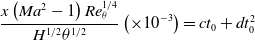 \begin{align}\frac{{x\left( {M{a^2} - 1} \right)Re_\theta ^{1/4}}}{{{H^{1/2}}{\theta ^{1/2}}}}\left( { \times {{10}^{ - 3}}} \right) = c{t_0} + dt_0^2\end{align}
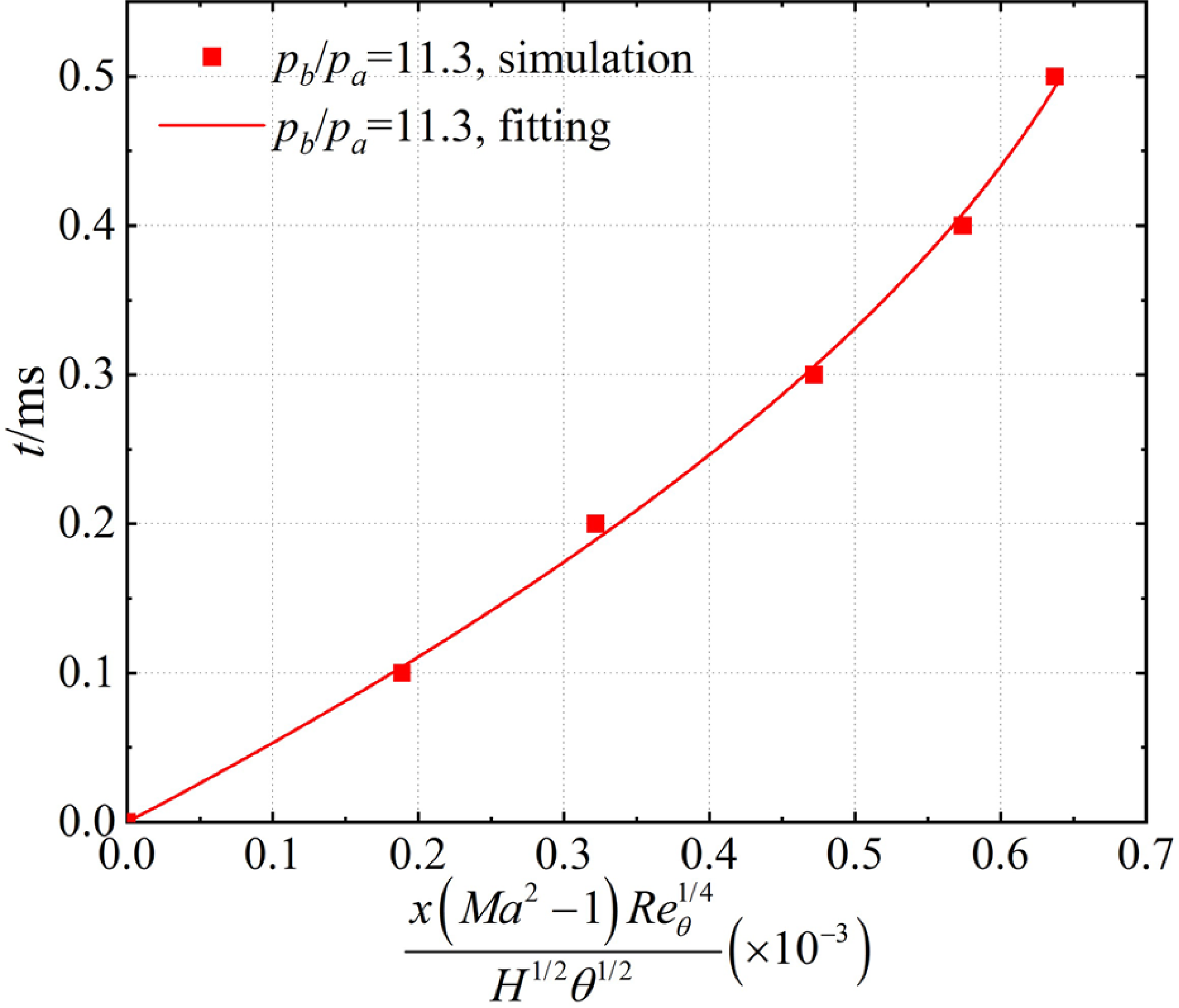
Figure 14. Backpressure duration and maximum backpropagation distance of BP1.1, BP2.1 and DT1.1–DT1.3.
Although the points appear to intersect with the curve roughly, it should be noted that the influence of changes in the backpressure peak has not been considered in the formula presented above. Specifically, since the backpressure peak in all five cases is the same, the relationship between $x$
and
$x$
and $c{t_0} + dt_0^2$
can be regarded as proportional. Therefore, it is essential to consider the potential impact of changes in backpressure peak when interpreting the results obtained from this formula. In doing so, a more comprehensive and accurate understanding of the relationship between
$c{t_0} + dt_0^2$
can be regarded as proportional. Therefore, it is essential to consider the potential impact of changes in backpressure peak when interpreting the results obtained from this formula. In doing so, a more comprehensive and accurate understanding of the relationship between $x$
and
$x$
and $c{t_0} + dt_0^2$
can be achieved.
$c{t_0} + dt_0^2$
can be achieved.
After the above analysis, we know that $x$
is proportional to
$x$
is proportional to $a\left( {{p_{b\_max}}/{p_a} - 1} \right) + b{\left( {{p_{b\_max}}/{p_a} - 1} \right)^2}$
and
$a\left( {{p_{b\_max}}/{p_a} - 1} \right) + b{\left( {{p_{b\_max}}/{p_a} - 1} \right)^2}$
and $c{t_0} + dt_0^2$
, respectively. It may be written as the product of the above two terms:
$c{t_0} + dt_0^2$
, respectively. It may be written as the product of the above two terms:
 \begin{align}\frac{{x\left( {M{a^2} - 1} \right)Re_\theta ^{1/4}}}{{{H^{1/2}}{\theta ^{1/2}}}}\left( { \times {{10}^{ - 3}}} \right) & = \prod\nolimits_1^n {{\sigma _i}{f_1}} \left( {\frac{{{p_{b\_max}}}}{{{p_a}}} - 1} \right){f_2}\left( {{t_0}} \right)\nonumber\\[9pt]& = \prod\nolimits_1^n {{\sigma _i}\left[ {a\left( {\frac{{{p_{b\_max}}}}{{{p_a}}} - 1} \right) + b{{\left( {\frac{{{p_{b\_max}}}}{{{p_a}}} - 1} \right)}^2}} \right]} \left( {c{t_0} + dt_0^2} \right)\end{align}
where ${\sigma _i}$
represents other backpressure characteristics that could influence the maximum backpropagation distance. For instance, we have also considered the influence brought by the moment pressure peak occurs, such as
${\sigma _i}$
represents other backpressure characteristics that could influence the maximum backpropagation distance. For instance, we have also considered the influence brought by the moment pressure peak occurs, such as $\left( {1/5} \right){t_0}$
,
$\left( {1/5} \right){t_0}$
, $\left( {1/3} \right){t_0}$
,
$\left( {1/3} \right){t_0}$
, $\left( {1/2} \right){t_0}$
,
$\left( {1/2} \right){t_0}$
, $\left( {2/3} \right){t_0}$
, and
$\left( {2/3} \right){t_0}$
, and $\left( {4/5} \right){t_0}$
. However, the results did not reveal significant variations in the maximum propagation distance among different cases. Consequently, the value of
$\left( {4/5} \right){t_0}$
. However, the results did not reveal significant variations in the maximum propagation distance among different cases. Consequently, the value of ${\sigma _i}$
brought by the moment pressure peak occurs is 1.
${\sigma _i}$
brought by the moment pressure peak occurs is 1.
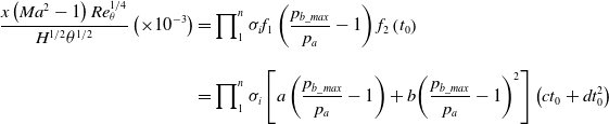
The data from BP1.0–2.1 and DT1.1–DT1.3 (represented by red scatter points in Fig. 16) were subjected to surface fitting to obtain the surface shown in Fig. 15. Specifically, the surface was generated to capture the relationship between the maximum backpropagation distance, the backpressure peak, and the backpressure duration. When considering the influence of ${p_{b\_max}}$
and
${p_{b\_max}}$
and ${t_0}$
, the value of
${t_0}$
, the value of $a$
,
$a$
, $b$
,
$b$
, $c$
, and
$c$
, and $d$
in the fitted surface equation was found to be –30.3, 64.0, 1.3, and –559.2, respectively. While the distribution trend of the blue scatter points (representing computational fluid dynamics (CFD) results of BP2.1–BP2.6) is roughly consistent with the surface, there remains a discrepancy due to the impact of other factors represented by
$d$
in the fitted surface equation was found to be –30.3, 64.0, 1.3, and –559.2, respectively. While the distribution trend of the blue scatter points (representing computational fluid dynamics (CFD) results of BP2.1–BP2.6) is roughly consistent with the surface, there remains a discrepancy due to the impact of other factors represented by ${\sigma _i}$
. To describe the distribution of the scatter points, the blue curve in Fig. 15 was obtained by setting
${\sigma _i}$
. To describe the distribution of the scatter points, the blue curve in Fig. 15 was obtained by setting ${t_0} = 0.2{\kern 1pt} {\kern 1pt} {\kern 1pt} {\kern 1pt} ms$
in Equation (16). Although this function provides an approximate description of the scatter points distribution, it is important to note that the fitting results can still be utilised to estimate the maximum backpropagation distance and to understand the effect of
${t_0} = 0.2{\kern 1pt} {\kern 1pt} {\kern 1pt} {\kern 1pt} ms$
in Equation (16). Although this function provides an approximate description of the scatter points distribution, it is important to note that the fitting results can still be utilised to estimate the maximum backpropagation distance and to understand the effect of ${p_{b\_max}}$
and
${p_{b\_max}}$
and ${t_0}$
on
${t_0}$
on $x$
.
$x$
.
Figure 15. CFD results and fitting surface.
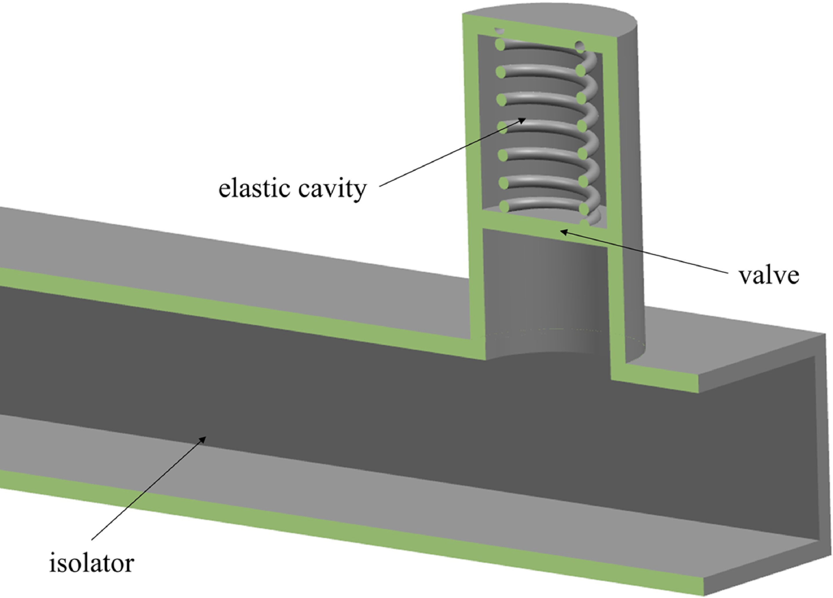
Figure 16. Elastic cavity at the outlet of isolator.
Overall, the fitting analysis provides information on the relationship between various factors that impact the maximum backpropagation distance, backpressure peak and backpressure duration. By understanding these relationships, we can develop improved strategies for controlling and mitigating backpressure effects in fluid systems.
The maximum backpropagation distance increases with increasing the backpressure peak when the backpressure duration is fixed. However, when the backpressure peak is fixed, the increasing rate of maximum backpropagation distance diminishes as the backpressure duration increases. This implies that when the integral of backpressure to time is constant, i.e., when the impulse generated by a single cycle of detonation combustion remains unchanged, reducing the backpressure peak and increasing the duration will result in a decrease in the backpressure pulsation at the outlet of the isolator. This reduction in pulsation will be more conducive to shortening the maximum backpropagation distance than reducing the duration and increasing the backpressure peak. For instance, the dimensionless maximum backpropagation distance of BP2.1, with a backpressure integral to time identical to that of BP1.6, is only 0.322, approximately 59.6% shorter than that of BP1.6.
The above idea suggests that a buffer device can be added between the isolator and combustor to convert the large-amplitude and short-duration pulse backpressure generated by detonation into a small-amplitude and long-duration pulse backpressure, which can effectively shorten the length of the isolator. One possible structure for the buffer device is shown in Fig. 16. The elastic cavity can be filled with inert gas or installed with a spring. When high pressure is generated in the combustor, the gas or spring in the elastic cavity is compressed by the movement of the valve, temporarily storing the pressure potential in the elastic cavity. As the pressure in the combustor decreases to the same level as that in the elastic cavity, the valve will gradually reset.
In summary, by reducing the backpressure peak and increasing the duration, the pulsation at the outlet of the isolator can be reduced, leading to a shorter maximum backpropagation distance. Additionally, the proposed buffer device could mitigate the adverse effects of the large-amplitude and short-duration pulse backpressure generated by detonation. It should be noted that the response time of the spring in the cavity mechanism should be less than the duration for one cycle of the combustor. For example, for a pulse detonation combustor with a working frequency of 100Hz, the response time of the spring should be less than 10ms.
5.0 Conclusions
In conclusion, the present study utilises transient CFD simulations to gain preliminary insight into the behaviour of shock train in straight pipes subjected to large amplitude and fast impact backpressure. The simulation parameters are derived from the detonation combustion case in the coupling model of the inlet, isolator and combustor, which operates at Mach 2.5 and an altitude of 11km. The findings indicate that the pressure disturbance in the isolator under pulse backpressure initially exists in the form of a normal shock, which gradually forms a shock train as it approaches the upstream end while moving towards the outlet. It is noteworthy that the pressure disturbance in the isolator exhibits an intense forcing-response lag. From the moment of the backpressure peak appearance, it takes 36 times the backpressure duration for the pressure disturbance to reach the upstream end.
Furthermore, the prediction law of shock train length based on the experimental data of steady backpressure is unsuitable for estimating the maximum backpropagation distance under pulse backpressure. Nevertheless, it is observed that the maximum backpropagation distance and backpressure peak follow a quadratic relationship similar to that of the steady backpressure case. Additionally, $x$
and
$x$
and ${t_0}$
also exhibit a quadratic relationship. Consequently, a similar fitting approach is adopted to determine
${t_0}$
also exhibit a quadratic relationship. Consequently, a similar fitting approach is adopted to determine $x$
,
$x$
, $\left( {{p_{b\_max}}/{p_a} - 1} \right)$
, and
$\left( {{p_{b\_max}}/{p_a} - 1} \right)$
, and ${t_0}$
, leading to the development of a function describing the maximum backpropagation distance, which considers the pulse backpressure peak and duration. This function can be utilised to analyse the impact of
${t_0}$
, leading to the development of a function describing the maximum backpropagation distance, which considers the pulse backpressure peak and duration. This function can be utilised to analyse the impact of ${p_{b\_max}}$
and
${p_{b\_max}}$
and ${t_0}$
on
${t_0}$
on $x$
, predict the maximum backpropagation distance in the isolator, and propose a potential solution for shortening the isolator length, namely, reducing the backpressure peak and increasing duration, thereby minimising the backpressure pulsation at the outlet of the isolator. It is important to note that only the influence of backpressure peak, duration, and peak occurrence time on
$x$
, predict the maximum backpropagation distance in the isolator, and propose a potential solution for shortening the isolator length, namely, reducing the backpressure peak and increasing duration, thereby minimising the backpressure pulsation at the outlet of the isolator. It is important to note that only the influence of backpressure peak, duration, and peak occurrence time on $x$
has been considered and verified in this study. There may be other factors that affect
$x$
has been considered and verified in this study. There may be other factors that affect $x$
, which will be considered in follow-up studies.
$x$
, which will be considered in follow-up studies.
In summary, the findings of this study provide valuable insights into the behaviour of shock train in straight pipes subjected to large amplitude and fast impact backpressure, which can inform the design and optimisation of the isolator in PDR.


