


1. Introduction
In response to the imperative for fundamental investigation into the characteristics of rotating flows and the optimisation of intricate technical or engineering systems, researchers have directed significant attention toward the study of such flows. In engineering applications, fluids often flow within rotating cavities, which serve as approximate simulations of components found in more intricate equipment. A typical geometric feature is a cavity formed between two disks. A wide range of configurations can be set up using disks with various fluids, physical properties, shapes, properties, rotation speeds and related boundary conditions (Owen & Rogers Reference Owen and Rogers1989). The most common configuration is a closed rotor–stator cavity, characterised by a stationary-disk boundary layer (referred to as the Bödewadt boundary layer for an infinitely large stationary disk) and a rotating-disk boundary layer (referred to as the von Kármán boundary layer for an infinitely large rotating disk), alongside a coexisting laminar–transitional–turbulent region in the boundary layer. Thus, such problems have also been demonstrated to be an effective way to investigate the instability of rotating flows and the turbulent characteristics with wall constraints and rotation (Saric, Reed & White Reference Saric, Reed and White2003; Launder, Poncet & Serre Reference Launder, Poncet and Serre2010; Martinand, Serre & Viaud Reference Martinand, Serre and Viaud2023; Alfredsson, Kato & Lingwood Reference Alfredsson, Kato and Lingwood2024).
In this type of flow, turbulence initially develops within the stationary-disk boundary layer, as was predicted from the stability analysis (Serre, Tuliszka-Sznitko & Bontoux Reference Serre, Tuliszka-Sznitko and Bontoux2004) and as confirmed through numerical simulations (Séverac et al. Reference Séverac, Poncet, Serre and Chauve2007; Severac & Serre Reference Severac and Serre2007; Makino, Inagaki & Nakagawa Reference Makino, Inagaki and Nakagawa2015; Gao & Chew Reference Gao and Chew2021), as well as experimental observations (Schouveiler et al. Reference Schouveiler, Le Gal, Chauve and Takeda1999; Schouveiler, Le Gal & Chauve Reference Schouveiler, Le Gal and Chauve2001; Cros et al. Reference Cros, Floriani, Le Gal and Lima2005; Poncet, Chauve & Schiestel Reference Poncet, Chauve and Schiestel2005). The rotating-disk boundary layer on the rotating-disk side was found to remain relatively stable and only becomes unstable at higher Reynolds numbers before transitioning to turbulence.
In terms of the behaviours of instability, the characteristics on both disks are consistent. Gregory, Stuart & Walker (Reference Gregory, Stuart and Walker1955) were the first to observe cross-flow instability with the spiral wave shape, attributed to inflection points in the radial velocity. Subsequently, Tatro & Mollo-Christensen (Reference Tatro and Mollo-Christensen1967) and Faller & Kaylor (Reference Faller and Kaylor1967) reported instability with circular wave shapes associated with the interaction of viscous forces and the Coriolis force, naming them type I and type II instabilities, respectively. Once initiated by perturbations, spiral waves persist and can be described by three crucial parameters: the azimuthal wavenumber  $m$, the radial wavenumber
  ${\alpha }$ and the temporal frequency
  $\omega$ (Lingwood Reference Lingwood1996; Serre, Del Arco & Bontoux Reference Serre, Del Arco and Bontoux2001; Serre et al. Reference Serre, Tuliszka-Sznitko and Bontoux2004; Queguineur, Gicquel & Staffelbach Reference Queguineur, Gicquel and Staffelbach2020). In contrast to spiral waves, capturing circular waves presents greater challenges. This difficulty arises because circular waves manifest at lower Reynolds numbers and have a tendency to dissipate rapidly in the absence of noise, which provides perturbation energy (Lopez et al. Reference Lopez, Marques, Rubio and Avila2009; Poncet, Serre & Le Gal Reference Poncet, Serre and Le Gal2009).
The occurrence of instability does not necessarily imply that the boundary layer on the disk will develop into turbulence. Lingwood (Reference Lingwood1995, Reference Lingwood1997) discovered a type III instability mode that rotates relative to the rotating disk. This instability mode combines with the type I instability when  $R_\delta \geq 507$ (
 ${R_{\delta }} = {r} \sqrt {{\varOmega }/{\nu }}$, where
  $r$ refers to the local radial position,
  $\varOmega$ represents the angular velocity of the disk and
  $\nu$ denotes kinematic viscosity) to form a type I absolute instability regime, inducing nonlinear effects that mark the onset of turbulent transition. However, type III instability has only been predicted through stability analysis in a rotating disk and has never been experimentally reported.
The existing research on the transition to turbulence in rotating flows is primarily based on single rotating disks (Lingwood Reference Lingwood1996; Pier Reference Pier2003, Reference Pier2007; Imayama, Alfredsson & Lingwood Reference Imayama, Alfredsson and Lingwood2014; Appelquist et al. Reference Appelquist, Schlatter, Alfredsson and Lingwood2016b, Reference Appelquist, Schlatter, Alfredsson and Lingwood2018; Lee et al. Reference Lee, Nishio, Izawa and Fukunishi2018; Thomas, Stephen & Davies Reference Thomas, Stephen and Davies2020), with only a limited amount of research focused on rotor–stator (Makino et al. Reference Makino, Inagaki and Nakagawa2015; Yim et al. Reference Yim, Chomaz, Martinand and Serre2018) and rotor–rotor (Viaud, Serre & Chomaz Reference Viaud, Serre and Chomaz2008, Reference Viaud, Serre and Chomaz2011) cavities. Two principal routes to turbulence have been proposed based on the nature of the dominant transition mechanisms, termed convective or absolute instability. While both pathways necessitate the existence of an absolutely unstable region with adequate radial extent, the former relies on external forcing whereas the latter is self-sustaining.
In the convective scenario, several sustained external perturbations are amplified through convection within the radial range of  $284 < R_\delta \cong 507$. When the perturbation, such as spiral waves, reaches nonlinear energy saturation before attaining its maximum radius, its convective instability transitions to an absolutely unstable state relative to secondary instabilities. This transition heralds the onset of localised turbulence (Pier Reference Pier2007). Several researchers have specifically investigated this scenario and have found that the amplitude of forced perturbations, as well as the roughness on the rotating disk in experiments, can affect the critical Reynolds number at which turbulence occurs (Appelquist et al. Reference Appelquist, Imayama, Alfredsson, Schlatter and Lingwood2016a; Imayama, Alfredsson & Lingwood Reference Imayama, Alfredsson and Lingwood2016; Thomas & Davies Reference Thomas and Davies2018; Thomas et al. Reference Thomas, Stephen and Davies2020). Additionally, when the radius of spiral waves extends sufficiently to be influenced by secondary global instabilities, local turbulence may promptly occur at the local or slightly downstream position (Appelquist et al. Reference Appelquist, Schlatter, Alfredsson and Lingwood2018).
The absolute scenario occurs when the region of absolute instability extends adequately before reaching the outer edge, and it entails the presence of spiral waves associated with relative disc motion (travelling mode) without any external perturbation. Depending on the flow conditions, this can be categorised into subcritical and supercritical scenarios. The supercritical scenario is driven by linear global instability, where infinitesimal initial perturbations can trigger linear global modes with steep fronts (Imayama, Alfredsson & Lingwood Reference Imayama, Alfredsson and Lingwood2013; Imayama et al. Reference Imayama, Alfredsson and Lingwood2014; Yim et al. Reference Yim, Chomaz, Martinand and Serre2018). The local absolute instability propels these modes at the radial edge of the disk. In contrast, the subcritical scenario is propelled by nonlinear global instability (Pier Reference Pier2003). In this case, the flow responds to strong impulse perturbations through steep global modes located at the upstream limit of the absolutely unstable zone, leading to local turbulence (Viaud et al. Reference Viaud, Serre and Chomaz2008, Reference Viaud, Serre and Chomaz2011; Yim et al. Reference Yim, Chomaz, Martinand and Serre2018).
In comparison with a single rotating disk, a rotor–stator cavity exhibits radial variations in flow velocity within the core region. Additionally, the boundaries of the boundary layer, including the casing and the shaft, serve as significant sources of disturbance. Significantly, in studies exploring the rotating-disk boundary layer within the cavity, such as Yim et al. (Reference Yim, Chomaz, Martinand and Serre2018), who investigated the stability of the rotating-disk boundary layer using direct numerical simulation, it was observed that the stationary-disk boundary layer had already transitioned to turbulence. There was no evidence to suggest that the intense turbulence within the stationary-disk boundary layer would not impact the transition to turbulence within the rotating-disk boundary layer (Martinand et al. Reference Martinand, Serre and Viaud2023). This inevitably led to consideration of the transition process in the stationary-disk boundary layer. While the destabilisation behaviours of the rotating- and stationary-disk boundary layers may appear analogous, it is noteworthy that the laminar–transition–turbulence coexistence within the stationary-disk boundary layer has not been documented, thus leaving the route to turbulence unclear.
As such, in the present study, the aim was to capture the coexistence of laminar–transition–turbulence on the stationary-disk boundary layer. Based on this, the aim was to identify a possible route leading to turbulence on the stationary-disk boundary layer. Reviewing existing articles on the presence of turbulence in the stationary-disk boundary layer in a rotor–stator cavity, the experimental results devoted to the stationary-disk boundary layer are few because there are more technical difficulties in studying it than the boundary layer of the rotor. Numerical simulations conducted by Serre et al. (Reference Serre, Del Arco and Bontoux2001) presented a range of disturbances. However, as time progressed, these disturbances either settled down or persisted in the form of spiral waves. The experiments conducted by Cros et al. (Reference Cros, Floriani, Le Gal and Lima2005) identify the occurrence of nonlinear interactions between circular and spiral modes, which result in the eventual transition to turbulence at moderate Reynolds numbers. However, they did not elucidate the sources of the disturbances on the stationary-disk boundary layer, nor did they provide a detailed account of how these disturbances evolve into turbulence. Further, this conclusion contradicts the findings of Lopez et al. (Reference Lopez, Marques, Rubio and Avila2009), who proposed minimal interaction between spiral and circular waves in their study. To address the described challenges, global stability analysis was employed in the present study (Barkley, Blackburn & Sherwin Reference Barkley, Blackburn and Sherwin2008). Initially, the unstable mode corresponding to a specific Reynolds number and azimuthal wavenumber was obtained. Subsequently, through a combination with direct numerical simulation (DNS), it became possible to capture the linear growth process of the perturbation eigenmode, nonlinear saturation and the emergence of localised turbulence. To accurately capture the development of the unstable characteristic mode at a specific azimuthal wavenumber (the current study focuses on  $m=32$), DNS is performed in a sector with an angle of
  $2{\rm \pi} /32$. This approach solely considers the azimuthal wavenumber
  $m=32$ and its harmonics, discussing the nonlinear interactions between these specific modes. Although many previous studies by Appelquist et al. (Reference Appelquist, Imayama, Alfredsson, Schlatter and Lingwood2016a), Appelquist et al. (Reference Appelquist, Schlatter, Alfredsson and Lingwood2018) and Lee et al. (Reference Lee, Nishio, Izawa and Fukunishi2018) have employed sectors of sizes
  $2{\rm \pi} /32$ and
  $2{\rm \pi} /68$ rad to investigate the transition pathways on the boundary layer, providing evidence on the use of sectors in DNS, it is important to note that the transition mechanism obtained under such a sector can only represent a possible mechanism of the rotor–stator cavity. While the nonlinear interactions among all modes may be also significant, such considerations lie beyond the scope of our current study.
The rest of the present paper is organised as follows. In § 2, the method and set-up of the simulations used in the present study are discussed. Results from global linear stability analysis and DNS are presented in § 3, and a discussion of these results is also included. Finally, § 4 provides a summary and conclusions
2. Method
In the present study, the Semtex code was utilised, a high-order numerical tool that combines Fourier and spectral element methods. This code, referenced in works by Barkley et al. (Reference Barkley, Blackburn and Sherwin2008) and Blackburn et al. (Reference Blackburn, Lee, Albrecht and Singh2019), implements a spatial discretisation technique that merges continuous-Galerkin nodal spectral elements with Fourier expansions. Specifically, it applies Fourier expansions along the azimuthal direction and spectral elements within the meridional  $(r, z)$ semiplane. For time integration, the code utilises a semi-implicit strategy employing a time-splitting scheme, ensuring that all simulations maintain second-order accuracy in time.
2.1. Governing equations
Under the assumption of a Newtonian fluid and incompressible flow, the governing equations for the primary variables (velocity and pressure) can be formulated as the incompressible Navier–Stokes equations
 \begin{equation} \frac{{{\partial} \boldsymbol{u}}}{{\partial t}} + {\boldsymbol{N}}(\boldsymbol{u}) ={-} \frac{1}{\rho }\boldsymbol{\nabla} p + \nu {{\nabla}^2}\boldsymbol{u}, \end{equation}
together with the continuity equation
 \begin{equation} \boldsymbol{\nabla} \boldsymbol{\cdot} \boldsymbol{u} = 0, \end{equation}
where  $\boldsymbol {u} = \boldsymbol {u} (r, \theta, z, t)$ is the velocity field,
  ${\boldsymbol {N}} (\boldsymbol {u})$ represents nonlinear advection terms,
  $p$ is the pressure,
  $\rho$ is the density and
  $\nu$ is the kinematic viscosity of the fluid. The variables
  $r, \theta, z$ and
  $t$ represent, the radial, azimuthal, axial and time coordinates, respectively, and
  $u, v$ and
  $w$ are the velocity components in the radial, azimuthal and axial directions. Here, we consider the nonlinear term in skew-symmetric form
  ${{\boldsymbol {N}} (\boldsymbol {u}) = (\boldsymbol {u} \boldsymbol{\cdot } \boldsymbol {\nabla } \boldsymbol {u} + \boldsymbol {\nabla } \boldsymbol{\cdot} \boldsymbol {u}\boldsymbol {u})/2}$.
If the velocity field exhibited a periodicity of  $L_\theta$ (in rad) in the azimuthal direction, a azimuthal wavenumber of fundamental component
  $\beta = 2{\rm \pi} /L_\theta$ was adopted. Consequently, it could be effectively decomposed into a set of two-dimensional complex Fourier modes, denoted as
 \begin{equation} {\boldsymbol{\hat u}_k}(r, z, t) = \frac{1}{{L_\theta }}\int_0^{L_\theta } {\boldsymbol{u}(r, z, \theta ,t)\,\mathrm{e}^{ - \mathrm{i}\beta k\theta }\,\mathrm{d}\theta }, \end{equation}
where  $k$ represents an integer wavenumber, and
  $\mathrm {i}$ is the unit imaginary number. In physical space, the azimuthal wavenumber
  $m$ is represented as
  $\beta k$. The velocity field has the associated Fourier series reconstruction
 \begin{equation} \boldsymbol{u}(r,\theta,z,t) = \sum_{k ={-} \infty }^\infty {{\hat{\boldsymbol u}_k}(r,z,t)\,\mathrm{e}^{\mathrm{i} \beta k\theta }}. \end{equation}
Thus, the cylindrical components of the transformed momentum equations (2.1) can be written
 \begin{gather} {\partial _t}{\hat u_k} + { {\hat{\boldsymbol{N}}(\boldsymbol{u})}_{rk}} ={-} \frac{1}{\rho }{\partial _r}{\hat p_k} + \nu \left(\nabla_{rz}^2 - \frac{{{k^2} + 1}}{{{r^2}}}\right){\hat u_k} - {\nu}\frac{{2\mathrm{i}k}}{{{r^2}}}{\hat v_k}, \end{gather}
 \begin{gather}{\partial _t}{\hat v_k} + {{\hat{\boldsymbol{N}}(\boldsymbol{u})}_{\theta k}} ={-} \frac{{\mathrm{i}k}}{{\rho r}}{\hat p_k} + \nu \left(\nabla_{rz}^2 - \frac{{{k^2} + 1}}{{{r^2}}}\right){\hat v_k} + {\nu}\frac{{2\mathrm{i}k}}{{{r^2}}}{\hat u_k}, \end{gather}
 \begin{gather}{\partial _t}{\hat w_k} + {{\hat{\boldsymbol{N}}(\boldsymbol{u})}_{zk}} ={-} \frac{1}{\rho }{\partial _z}{\hat p_k} + \nu \left(\nabla_{rz}^2 - \frac{{{k^2}}}{{{r^2}}}\right){\hat w_k}, \end{gather}
where  ${{\hat {\boldsymbol {N}}(\boldsymbol {u})}_{rk}}, {{\hat {\boldsymbol {N}}(\boldsymbol {u})}_{\theta k}}$ and
  ${{\hat {\boldsymbol {N}}(\boldsymbol {u})}_{zk}}$ represent mode-
 $k$ components of the transformed nonlinear terms. Here,
  $\nabla _{rz}^2$ is related to the Laplacian function of the mode
  $k$ under Fourier decomposition
 \begin{equation} \nabla_{rz}={\partial^2_z}+\frac{1}{r}{\partial _r}(r{\partial _r}). \end{equation}
To decouple the linear terms, a change of variables can be introduced as  ${\tilde u_k} = {\hat u_k} + \mathrm {i}{\hat v_k}$ and
  ${\tilde v_k} = {\hat u_k} - \mathrm {i}{\hat v_k}$ (Lopez, Marques & Shen Reference Lopez, Marques and Shen2002), following the approach described by Orszag (Reference Orszag1974) in the context of Fourier decompositions. This change of variables yields the following expressions for the equations:
 \begin{gather} {\partial _t}{\tilde u_k} + {{\tilde{\boldsymbol{N}}(\boldsymbol{u})}_{rk}} ={-} \frac{1}{\rho }\left({\partial _r} - \frac{k}{r}\right){\hat p_k} + \nu \left(\nabla_{rz}^2 - \frac{{{{(k + 1)}^2}}}{{{r^2}}}\right){\tilde u_k}, \end{gather}
 \begin{gather}{\partial _t}{\tilde v_k} + {{\tilde{\boldsymbol{N}}(\boldsymbol{u})}_{\theta k}} ={-} \frac{1}{\rho }\left({\partial _r} + \frac{k}{r}\right){\hat p_k} + \nu \left(\nabla_{rz}^2 - \frac{{{{(k - 1)}^2}}}{{{r^2}}}\right){\tilde v _k}, \end{gather}
 \begin{gather}{\partial _t}{\hat w_k} + {{\hat{\boldsymbol{N}}(\boldsymbol{u})}_{zk}} ={-} \frac{1}{\rho }{\partial _z}{\hat p_k} + \nu \left(\nabla_{rz}^2 - \frac{{{k^2}}}{{{r^2}}}\right){\hat w_k}, \end{gather}
where  ${{\tilde {\boldsymbol {N}}(\boldsymbol {u})}_{rk}} = {{\hat {\boldsymbol {N}}(\boldsymbol {u})}_{rk}} + {\rm {i}}{{\hat {\boldsymbol {N}}(\boldsymbol {u})}_{\theta k}}$ and
  ${{\tilde {\boldsymbol {N}}(\boldsymbol {u})}_{\theta k}} = {{\hat {\boldsymbol {N}}(\boldsymbol {u})}_{rk}} - {\rm {i}}{{\hat {\boldsymbol {N}}(\boldsymbol {u})}_{\theta k}}$.
When analysing the global linear stability of a flow in terms of its normal modes, the pressure was considered as the solution of a Poisson equation with the divergence of the advection terms as the forcing. In this context, the Navier–Stokes equations can be represented symbolically as follows:
 \begin{equation} \frac{{\partial \boldsymbol{u}}}{{\partial t}} ={-} {({\boldsymbol{I}} - \boldsymbol{\nabla} {\nabla^{ - 2}}\boldsymbol{\nabla}\,\boldsymbol{\cdot}\,)\boldsymbol{N}(\boldsymbol{u})} + \nu {\nabla^2}\boldsymbol{u} = {\boldsymbol{A}(\boldsymbol{u}) + {\boldsymbol{L}}(\boldsymbol{u})}. \end{equation}
The nonlinear operator  $\boldsymbol {A}(\boldsymbol {u})$ includes contributions from advection and pressure terms, while the linear operator
  ${\boldsymbol {L}}(\boldsymbol {u})$ corresponds to viscous diffusion. It is worth noting that, while opting for a skew-symmetric form of the nonlinear term in DNS, it is susceptible to numerical instability in global linear stability analysis (Wilhelm & Kleiser Reference Wilhelm and Kleiser2001). Consequently, in global linear stability analysis, the nonlinear term
  ${\boldsymbol {N}(\boldsymbol {u})}$ is modelled in a convective form
  $\boldsymbol {u} \boldsymbol{\cdot} \boldsymbol {\nabla } \boldsymbol {u}$ (Barkley et al. Reference Barkley, Blackburn and Sherwin2008). The velocity
  $\boldsymbol {u}$ can be decomposed into a base flow
  $\boldsymbol {U}$ and a perturbation flow
  $\boldsymbol {u}'$. In this decomposition, the original nonlinear advection terms are replaced with their linearised equivalent
  ${\boldsymbol {N}_{\boldsymbol {U}}}(\boldsymbol {u}') = \boldsymbol {U} \boldsymbol{\cdot} \boldsymbol {\nabla } \boldsymbol {u}' + \boldsymbol {u}' \boldsymbol{\cdot} \boldsymbol {\nabla } \boldsymbol {U}$. The linearised equivalent of (2.12) for an infinitesimal perturbation
  $\boldsymbol {u}'$ can be written as
 \begin{equation} {\partial_t}\boldsymbol{u}' = \boldsymbol{A}_{\boldsymbol{U}}(\boldsymbol{u}') + \boldsymbol{L}(\boldsymbol{u}'), \end{equation}
where  $\boldsymbol {A}_{\boldsymbol {U}}(\boldsymbol {u}')$ represents the linearisation (Jacobian) of
  $\boldsymbol {A}(\boldsymbol {u}')$ about the base flow
  $\boldsymbol {U}$.
Under the assumption of normal modes,  $\boldsymbol {u}'(t) \equiv \tilde {\boldsymbol {u}}\mathrm {e}^{\lambda t}$, (2.13) can be transformed into an eigenproblem
 \begin{equation} \lambda \boldsymbol{\tilde u} = ({\boldsymbol{A}_{\boldsymbol{U}}(\boldsymbol{u}') + \boldsymbol{L}(\boldsymbol{u}')})\boldsymbol{\tilde u}, \end{equation}
where  $\lambda$ is the eigenvalue and
  $\boldsymbol {\tilde u}$ is its eigenfunction, both typically appearing in complex-conjugate pairs. For a finite time increment
  $\tau$, this can be expressed as follows:
 \begin{equation} \boldsymbol{u}'(t_0+\tau)=\exp[(\boldsymbol{A}_{\boldsymbol{U}}(\boldsymbol{u}')+\boldsymbol{ L}(\boldsymbol{u}'))\tau]\boldsymbol{u}'(t_0). \end{equation}
The aim is to extract the eigenpairs ( $\varGamma, \boldsymbol {\tilde u}$) of the operator
  $(\boldsymbol {A}_{\boldsymbol {U}}(\boldsymbol {u}')+\boldsymbol { L}(\boldsymbol {u}'))\tau$. This is crucial because the numerical method employed generally identifies dominant eigenvalues, which are those with the largest magnitude. However, for steady flow, the primary focus was on the values of
  $\lambda$ with the largest real part, indicating the most unstable behaviour. There is a direct correspondence between the dominant values of
  $\varGamma$ and the most unstable values of
  $\lambda$ through the relation
  $\varGamma = \mathrm {e}^{\lambda {\Delta } t}$. Note that, in carrying out the time interval,
  $\tau = n{\Delta } t$,
  $n$ is a larger finite integer (Tuckerman & Barkley Reference Tuckerman and Barkley2000).
2.2. Simulation set-up
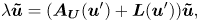
In the present investigation, the adopted geometric configuration is akin to prior studies conducted by Lopez et al. (Reference Lopez, Marques, Rubio and Avila2009), Peres, Poncet & Serre (Reference Peres, Poncet and Serre2012) and Yim et al. (Reference Yim, Chomaz, Martinand and Serre2018). The configuration comprises two vertical disks with a radius of  $R$, enclosed by a shroud represented by a vertical cylinder of width
  $2H$. The rotor and the cylinder rotate at an angular velocity of
  $\varOmega$ while the stator remains stationary. A schematic diagram of the flow system is presented in figure 1. The cavity aspect ratio, defined as the ratio of
  $R$ to
  $H$, is fixed at
  $10.26$. The characteristic Reynolds number is defined as
  ${{Re}} = \varOmega R^2 / \nu$.
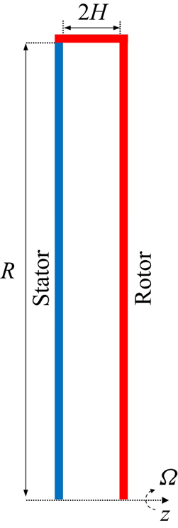
Figure 1. A sketch of the computational domain for rotor–stator cavity flow. Here,  $\varOmega$ is the angular velocity,
  $2H$ is the distance between stator and rotor and
  $R$ represents the radius of the shroud. The rotor rotates along with the shroud.
The spectral element mesh has 800 elements, and tensor products of sixth-order Gauss–Lobatto–Legendre Lagrange shape functions are used within each element, providing a total of 28800 independent mesh points in the discretisation of the meridional  $(r, z)$ semiplane. In the azimuthal direction of the three-dimensional DNS, we have chosen the fundamental wavenumber
  $\beta = 32$, which corresponds to a sector of an angle of
  $2{\rm \pi} /32$ rad. Therefore, the relationship between the azimuthal wavenumber
  $m$ in the physical space and the Fourier mode
  $k$ in the direct numerical simulation can be expressed as
  $m = \beta k = 32k$ . After verification, it was determined that using 48 Fourier planes provided sufficient accuracy for the current problem. Therefore, 48 Fourier planes were chosen for DNS, corresponding to a total of 24 Fourier modes.
No-slip boundary conditions are enforced at the stator and rotor interfaces:  $u = w = 0$, while the azimuthal velocity
  $v = 0$ on the stationary disk and
  $v = \varOmega r$ on the rotating disk and rotating shroud. The rotation induced by the rotating shroud ensures a stable inflow within the stationary-disk boundary layer, effectively mitigating additional disturbances and thereby enhancing the accuracy of the results in the global linear stability analysis. At the junction of the rotating shroud with the stator, the azimuthal velocity profile is regularised using
 \begin{equation} v = \varOmega r(1 - \mathrm{e}^{ - {z/( {H + 1})}/{{0.006}}}), \end{equation}
where the value 0.006 was shown to accurately model the velocity profiles observed in experiments (Serre et al. Reference Serre, Del Arco and Bontoux2001). On the cylinder axis ( $r=0$), boundary conditions are wavenumber dependent
 \begin{equation} \left. \begin{aligned} k = 0,{\partial _r}{\hat w_0} = \tilde u_0^{{\dagger}} = {\tilde v_0} = {\partial _r}{\hat p_0} = 0\\ k =1,\hat w_1^{{\dagger}} = \tilde u_1^{{\dagger}} = {\partial _r}{\tilde v_1} = \hat p_1^{{\dagger}} = 0\\ k > 1,\hat w_k^{{\dagger}} = \tilde u_k^{{\dagger}} = \tilde v_k^{{\dagger}} = \hat p_k^{{\dagger}} = 0 \end{aligned} \right\},\ \mathrm{at} \ r = 0. \end{equation}
Here, the superscript  ${{\dagger}}$ indicates the essential pole boundary conditions, and the remaining terms are derived from parity requirements. For specific details, please refer to Lopez et al. (Reference Lopez, Marques and Shen2002) and Blackburn & Sherwin (Reference Blackburn and Sherwin2004). For the global linear stability analysis, the boundary perturbation velocity
  $\boldsymbol {u}'$ was set to zero, while a high-order Neumann boundary condition was applied to the perturbation pressure (Karniadakis, Israeli & Orszag Reference Karniadakis, Israeli and Orszag1991).
The two-dimensional (2-D) DNS provided the base flow on the meridional  $(r, z)$ semiplane at the specific Reynolds number for stability analysis. Due to the fact that the Fourier mode
  $k=0$ in 2-D simulations is not affected by any
  $k\ne 0$ modes, this implies that referring to the results of 2-D DNS as the base flow is more appropriate. Sipp & Lebedev (Reference Sipp and Lebedev2007) specifically emphasised that the base flow and mean flow can lead to different stability analysis results. After comparing the results of global linear stability analysis, a sixth-order polynomial distribution was ultimately adopted, and the time interval
  $\tau =2/\varOmega$ was divided into 2000 time steps
  $\Delta t$. The initial velocity distribution for the 3-D DNS were obtained by linearly superimposing the most unstable mode
  $k=32$ obtained from stability analysis with the base flow. For all DNS, the time step satisfied
  $\Delta t = {{2{\rm \pi} }}/{{(6280\varOmega )}}$.
3. Results
3.1. Base flow characteristics
The main characteristics of the steady base flow are indicated in figure 2, in which dimensionless radial, azimuthal and axial velocity profiles for the flow at  ${{Re}} = 1.2 \times {10^5}$ are presented. Unless otherwise specified, all meridional
  $(r, z)$ semiplane plots in the present paper depict the left side representing the stator and the right side representing the rotor. As depicted in figure 2(a), most of the cavity exhibited axial flow directed from the stator towards the rotor. However, at the outermost radial position, the presence of the shroud induced a redirection of the flow, causing it to move from the rotor towards the stator, effectively simulating an inflow originating from the stator. The entire cavity encompassed three distinct boundary layers: the stationary-disk boundary layer, the rotating-disk boundary layer and the boundary layer at the shroud. Figure 2(a) provides a clear visualisation of the extent of these boundary layers on both the stator and rotor sides. An inviscid core within the cavity separated these two boundary layers, while the boundary layer at the shroud exhibited characteristics resembling a Stewartson boundary layer (Poncet et al. Reference Poncet, Serre and Le Gal2009). In figure 2(b), the non-dimensionalised azimuthal velocity component
  $v/(\varOmega r)$ increases with the radial position. Particularly near the shroud, the azimuthal velocity was nearly two orders of magnitude greater than the radial and axial velocities. This characteristic permitted a reasonable approximation of the flow as an axisymmetric flow with a dominant velocity component of (0,
  $v(r)$, 0). Moreover, the azimuthal velocity exhibited a positive gradient for the radial position (i.e.
  ${\textrm {d}}(vr)/\textrm {d}r > 0$). Applying the Rayleigh stability criterion, this flow configuration could be considered stable against inviscid, axisymmetric disturbances (Sipp & Jacquin Reference Sipp and Jacquin2000). The stationary-disk boundary layer at the shroud is deemed stable. Additionally, it is apparent from figure 2(c) that the axial velocity component
  $w/(\varOmega R)$ demonstrated a considerably lower magnitude, approximately two orders of magnitude lower than the other two velocity components, and it tended toward zero. Therefore, this observation prompted us to utilise the axial velocity as a representative parameter to characterise the perturbation in the subsequent analysis.
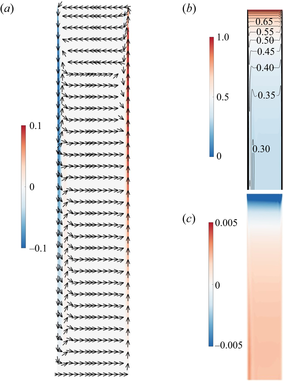
Figure 2. Two-dimensional DNS at  ${Re} = 1.2 \times {10^5}$. (a) Contour plots of dimensionless radial velocity
  ${{u}}/(\varOmega R)$ and vector field, (b) contour plots of dimensionless azimuthal velocity
  ${{v}}/(\varOmega r)$ and (c) axial velocity
  ${{w}}/(\varOmega R)$ on the meridional
  $(r, z)$ semiplane.
Figures 3(a) and 3(b) display the axial distribution of the radial velocity  $u/(\varOmega r)$ at the radius
  $r/H = 5.13$ in the stationary-disk boundary layer and the rotating-disk boundary layer, respectively. Unlike the radial velocity on the rotating-disk boundary layer, which decreased almost monotonically from its maximum value within the rotating-disk boundary layer, the stationary-disk boundary layer exhibited multiple inflection points, which inevitably rendered the stationary-disk boundary layer more prone to the development of inviscid cross-flow instability (Schwiderski & Lugt Reference Schwiderski and Lugt1964).
Figure 3. Two-dimensional DNS at  ${Re} = 1.2 \times {10^5}$. Profiles of the radial velocity
  $u/(\varOmega r)$ at
  $r/H=5.13$ in the (a) stationary-disk boundary layer, and (b) rotating-disk boundary layer.
3.2. Global linear stability analysis
Figure 4(a) illustrates the variation of the linear growth rate. This contour plot was composed of 452 data points, representing the growth rates  $\lambda _r$ of the most unstable mode for various azimuthal wavenumbers
  $m$ at Reynolds numbers ranging from
  $0.6 \times 10^5$ to
  $1.5 \times 10^5$.
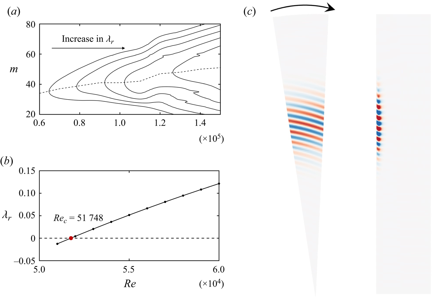
Figure 4. Results of global linear stability analysis. (a) The variation of the linear growth rate of the most unstable mode  $\lambda _r$ with azimuthal wavenumber
  $m$ for different Reynolds numbers
  $Re$. The solid lines from left to right represent
 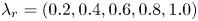 $\lambda _r = (0.2, 0.4, 0.6, 0.8, 1.0)$. The dashed represents the azimuthal wavenumber
  $m$ corresponding to the Reynolds number
  $Re$ with the maximum growth rate. (b) The growth rate
  $\lambda _r$ at different Reynolds numbers
  $Re$ for
  $m = 32$. (c) The visual representation of the most unstable mode of the base flow at
  $Re = 1.2 \times 10^5$ and
  $m=32$, the arrows indicate the direction of fluid rotation. The colour is consistent with figure 2(c), where the axial perturbation velocity
  $w'$ ranges from negative (blue) to positive (red).
Figure 4(a) is a contour plot interpolated from the linear growth rates  $\lambda _r$ derived from global linear stability analysis across 452 sets of (
 $Re$,
$Re$,  $m$), with the Reynolds number ranging from
  $0.6 \times 10^5$ to
  $1.5 \times 10^5$. Arrows on the plot indicate the direction of increasing
  $\lambda _r$. Owing to the global linear stability analysis being conducted in the Krylov subspace (Barkley et al. Reference Barkley, Blackburn and Sherwin2008), for a given Reynolds number
  $Re$ and azimuthal wavenumber
  $m$, multiple eigenmodes with a positive linear growth rate (
 $\lambda _r > 0$) may exist. Here, we consider only the eigenmode with the largest
  $\lambda _r$. As the Reynolds number increased, the maximum linear growth rate occurred at larger azimuthal wavenumbers. As depicted by the dashed line in figure 4(a), it represents the azimuthal wavenumber
  $m$ at which the growth rate
  $\lambda _r$ reached the maximum for each Reynolds number. When
  $Re=0.6\times 10^5$, the azimuthal wavenumber
  $m=32$ exhibited the highest growth rate. According to Lopez et al. (Reference Lopez, Marques, Rubio and Avila2009),
  $m=32$ corresponds to the azimuthal wavenumber at the critical Reynolds number. Therefore,
  $m=32$ was selected for the global stability analysis across the Reynolds number range from
  $0.51 \times 10^5$ to
  $0.6 \times 10^5$, and the results are shown in figure 4(b). This result is mainly consistent with Lopez et al.'s (Reference Lopez, Marques, Rubio and Avila2009) findings. In his model with a geometric parameter of
  ${R}/{H}=10$, a critical Reynolds number of
  $Re_c=51735$ was obtained when the azimuthal wavenumber
  $m=32$. Using cubic spline interpolation, the critical Reynolds number for the linearised perturbation growth at
  $m=32$ was obtained as
  $Re_c=51748$ in the present study. Figure 4(c) presents the 3-D structure of the perturbation eigenmode when
  $m=32$ and
  $Re=1.2 \times 10^5$. From left to right, the images represent the axial perturbation velocity
  $w'$ near the stationary-disk side at
  $z/H=-0.98$ and on the meridional
  $(r, z)$ semiplane. The perturbation eigenmode mainly occupies the radial position of
  $4 < r/H < 8$, with an average radial wavelength of 13
 $\delta$, where
  $\delta = \sqrt {{\nu /\varOmega }}$. This radial wavelength is shorter than those obtained through linear stability analysis by Serre et al. (Reference Serre, Tuliszka-Sznitko and Bontoux2004) and Lingwood (Reference Lingwood1997). This is due to the higher Reynolds number, which leads to a smaller radial wavelength of the spiral waves. A similar phenomenon was observed in the study by Yim et al. (Reference Yim, Chomaz, Martinand and Serre2018), where the radial wavelength of the spiral waves in the rotating-disk boundary layer decreased from
  $25.5\delta$ at
  $Re=1.76\times 10^5$ to
  $15.6\delta$ at
  $Re=2.9\times 10^5$.
In previous research (Serre et al. Reference Serre, Tuliszka-Sznitko and Bontoux2004), spiral waves were precisely defined via local stability analysis, and diverse characteristic parameters, such as the radial wavelength and frequency of spiral waves, were scrutinised. However, due to notable disparities in the base flow, reflecting stability characteristics at various radial positions, particularly at mid to high radii, establishing a suitable reference base flow to establish a meaningful correlation between the outcomes of the current global stability analysis and the analysis of local stability poses a significant challenge. As such, the present study does not incorporate a comparison with existing results from local stability analysis.
3.3. Direct numerical simulation
Global linear stability analysis provides the perturbation eigenmode that exhibits linear growth characteristics. However, understanding the nonlinear behaviour following linear growth and predicting the occurrence of local turbulence necessitates the adoption of DNS. By adding a small perturbation eigenmode to the base flow as the initial conditions, 3-D DNS could be initiated to explore the evolution of nonlinear behaviour. In the present study, the initial perturbation eigenmode energy was set to be  ${10}^{-10}$ of the base flow.
Here, for all DNS in the present study, the spiral eigenmode with azimuthal wavenumber  $m = 32$ was also selected without losing generality. As an important prerequisite, the present study concentrates on a fundamental instability mechanism related to eigenmodes. It is the primary instability spiral mode that distorts the base flow and admits transition. In this viewpoint, the chosen spiral mode is just a representative to illustrate this mechanism. The choice of the azimuthal wavenumber
  $m$ at a given
  $Re$ was relatively non-decisive. In addition, it is convenient to compare with other works and validate our observations and analysis, we chose
  $m = 32$, which is commonly used in the existing literature and represents the most unstable azimuthal wavenumber at the current critical Reynolds number
  $Re_c$.
Figure 5 displays the results of DNS at  $Re=1.2 \times 10^5$. The solid lines are the dimensionless amount of flow kinetic energy contained in each Fourier mode
  $k$
$k$
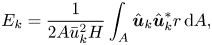 \begin{equation} {E_{{k}}} = \frac{1}{{2A\bar u_k^2}H}\int_A {{{\hat{\boldsymbol{u}}}_k}} \hat{\boldsymbol{u}}_k^*r\, {\rm d} A, \end{equation}
where  $A$ is the area of the 2-D meridional
  $(r, z)$ semiplane,
  $\bar u_k = \varOmega H$ and
  $\hat {\boldsymbol {u}}_k^*$ denotes the complex conjugate of the velocity data in the
  $k_{th}$ Fourier mode. The azimuthal wavenumber
  $m$ corresponding to these Fourier modes is given by
  $m = 32k$. The dotted line in figure 5 indicates the exponential growth for azimuthal wavenumber
  $m = 32$ (
 $k=1$ in the DNS), as predicted from the global linear stability analysis, and closely aligns with the DNS results.
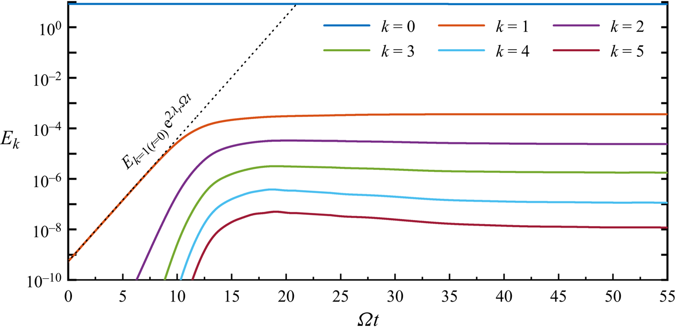
Figure 5. Growth to saturation at  $Re = 1.2 \times 10^5$, represented by kinetic energies in Fourier modes. The dotted line indicates the exponential growth rate for azimuthal wavenumber
  $m = 32$ (
 $k=1$ in the DNS).
The final simulation results of  $Re=1.2 \times 10^5$ ultimately reached a relatively stable state. However, in addition to this, the simulations of
  $Re=1.5 \times 10^5$ exhibited localised turbulence after sufficient development.
3.4. Discussion
3.4.1. Linear growth and nonlinear saturation
In figure 5, it is evident that all modes displayed a distinct phase characterised by linear energy amplification within a specific temporal window. Subsequently, this phase of linear global instability underwent a transition into nonlinear energy amplification at approximately  $\varOmega t=8$ rad, ultimately culminating in saturation around
  $\varOmega t=15$ rad. When
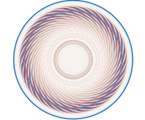
  $\varOmega t=45$ rad, in addition to the spiral waves resulting from inviscid instability, circular waves were also generated within the boundary layer due to the combined effects of viscosity and the Coriolis force. Existing literature substantiates that these circular waves propagate radially inward and lack the self-sustaining characteristics observed in spiral modes (Schouveiler et al. Reference Schouveiler, Le Gal, Chauve and Takeda1999, Reference Schouveiler, Le Gal and Chauve2001; Lopez et al. Reference Lopez, Marques, Rubio and Avila2009). Figure 6 displays instantaneous axial velocity
  $w/\varOmega R$ contour plots corresponding to linear growth (
 $\varOmega t=8$ rad), nonlinear saturation (
 $\varOmega t=15$ rad) and the coexistence of circular waves and spiral waves (
 $\varOmega t=45$ rad), respectively. In comparison with the perturbation eigenmode in figure 4(b), during the linear growth phase, the spiral waves exhibited minimal positional migration. The increase in perturbation velocity of the spiral waves reflects the linear growth of their energy. Since the inflow on the stationary-disk boundary layer was highly stable, with no disturbances present, perturbations at the high radial positions of the stationary-disk boundary layer originated from the nonlinear growth of spiral waves. That is, when nonlinear energy growth occurred, spiral waves simultaneously transmitted perturbation energy upstream (towards a higher radius) and downstream. Finally, circular waves appeared at smaller radial positions and occupied all the lower radial positions. As a result, nearly the entire boundary layer became perturbed.
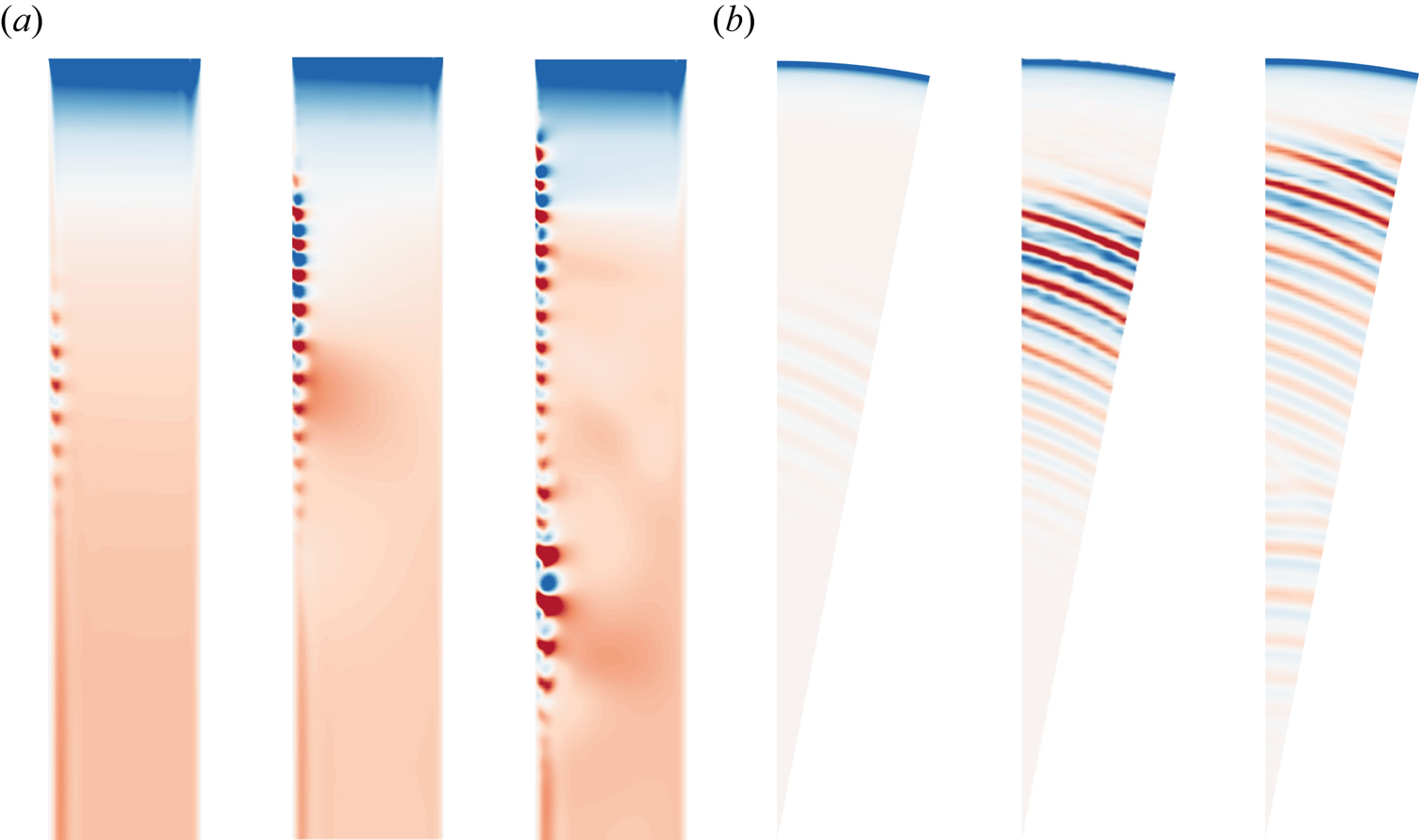
Figure 6. The visual representation of DNS at  $Re = 1.2 \times 10^5$. (a) Meridional
  $(r, z)$ semiplane. (b) Plane at
  $z/H=-0.98$. Here,
  $\varOmega t=8$ rad (left),
  $\varOmega t=15$ rad (middle) and
  $\varOmega t=45$ rad (right). The colour is consistent with figure 2(c), where the dimensionless axial velocity
  $w/(\varOmega R)$ ranges from -0.005 (blue) to 0.005 (red).
Owing to the radial constraints in the cavity, the spiral waves could not propagate endlessly upstream. Nonetheless, the upstream region corresponded to an area with higher local Reynolds numbers, making disturbances in its vicinity the most energetic throughout the boundary layer. This observation was clearly reflected in the vibrant colours observed in the upstream sector of figure 6. In previous investigations of the rotating-disk boundary layer, it has been noted that, when the radial extent is sufficiently large, whether due to convective instability or local absolute instability, spiral waves tend to induce localised turbulence downstream in the high-radius region. However, for the stationary-disk boundary layer, it is not yet clear whether it is due to further development of the spiral waves in the radial range, leading to localised turbulence in the boundary layer. This aspect will be further discussed later on.
The radial space–time plot in figure 7(a) illustrates the temporal evolution of the flow field at the position where  $z/H=-0.98, \theta =0$. Apart from linear growth and nonlinear saturation phenomena, circular waves developed when
  $\varOmega t = 25$ rad. Under the current Reynolds number, circular waves emerged from the mid-radius position and propagated downstream. During the time interval depicted in the figure, the initial radial position of the circular waves gradually decreased. The green dashed line and arrow in the figure emphasise this phenomenon, indicating that the circular waves would diminish over time. Notably, the phase velocities of different circular waves propagating downstream were inconsistent, which could result in the merging of circular waves. The green circle in the figure highlights this phenomenon. Results not presented here indicate that, even after undergoing 20 rotations of the rotating disk, circular waves persist and gradually dissipate. Compared with the results of Lopez et al. (Reference Lopez, Marques, Rubio and Avila2009), the current decay rate was very slow. In their study, they proposed that sudden changes in
  $Re$ led to the appearance of circular waves, largely attributed to changes in the mean flow. In the present research, it was observed that the saturation of spiral waves also led to variations in the mean flow. This correlation provided a possible explanation for the occurrence of circular waves in the present investigation. In a study by Lopez et al. (Reference Lopez, Marques, Rubio and Avila2009), with
  $Re=0.5\times 10^5$, the mean flow quickly stabilised, resulting in the rapid decay of circular waves within a short period of time. Contrastingly, in the present study, the mean flow continued to evolve after the saturation of spiral waves, which explains why the present circular waves persisted for a much longer duration compared with those in the study conducted by Lopez et al. (Reference Lopez, Marques, Rubio and Avila2009).
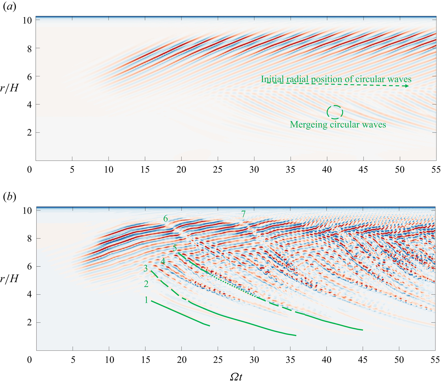
Figure 7. (a) Space–time plot showing  $w/\varOmega R$ at
  $z/H=-0.98$,
  $\theta = 0$ for
  $Re = 1.2 \times {10^5}$. (b) Space–time plot showing
  $w/\varOmega R$ at
  $z/H=-0.98$,
  $\theta =0$ for
  $Re = 1.5 \times {10^5}$. The colour is consistent with figure 2(c), where the dimensionless axial velocity
  $w/(\varOmega R)$ ranges from -0.005 (blue) to 0.005 (red).
3.4.2. The interference between spiral waves and circular waves and the generation of local turbulence
When conducting DNS at a higher Reynolds number, specifically  $Re=1.5 \times 10^5$, the observed linear growth patterns and subsequent nonlinear energy saturation closely resembled those observed at
  $Re=1.2 \times 10^5$. Nonetheless, owing to the elevated local Reynolds numbers associated with the high-radius region, the boundary layer manifests more complex disturbance behaviour following the nonlinear energy saturation.
The radial space–time plot depicted in figure 7(b) reveals that the earliest formation of circular wave structures occurred at  $\varOmega t=15$ rad. Additionally, multiple circular waves were observed between
  $r/H=4$ and
  $r/H=6$, denoted by the numbers 1, 2 and 3 in figure 7(b). These three circular waves exhibited similarities in terms of temporal and spatial scales. Their main characteristics in the space–time diagram are solid green lines. The only distinction is that wave 3 emerges at a higher radial position, resulting in its interaction and interference with the pre-existing spiral waves in terms of spatial localisation. As a result, this interference manifests as discontinuous structures during the initial phase of wave 3, as shown by the green dashed line in the space–time diagram. Subsequently, circular waves 4 and 5, appearing at higher radial positions, exhibited a more complex flow dynamics than the preceding waves. Initially, they interacted with the spiral waves, giving rise to disturbances with larger temporal and spatial scales. As they merged with other circular waves during downstream propagation, they swiftly induced high-frequency, small-scale perturbations in the flow field. Figure 7(a) also shows this merging phenomenon. However, specific small-scale vortices are not observed due to the absence of spiral waves at their intersection locations. Continuity was restored when the high-frequency, small-scale perturbations reached extremely low radial positions. Green dotted lines correspondingly illustrate the characteristics of these high-frequency, small-scale structures in the space–time diagram. While these circular waves interacted to different extents with the spiral waves, causing further disturbances in the boundary layer, their frequencies of occurrence and the radial range they affected were relatively small. As a result, the boundary layer could still revert to a relatively stable state.
As circular waves originating from higher radial positions propagated downstream, they interfered with the spiral waves throughout the entire boundary layer. Waves 6 and 7 emerged from the highest radial position of the spiral waves, and their initial interference with the spiral waves did not result in strong disturbances. During the downstream convective process, when they merged with other circular wave disturbances, they exhibited high-frequency small-scale perturbations similar to waves 4 and 5.
The present evidence suggests that, at  $Re=1.5\times 10^5$, besides the development of nonlinear saturated spiral waves, the interaction between circular waves and spiral waves led to additional disturbances in the boundary layer and the formation of small-scale perturbation structures. Starting from
  $\varOmega t=40$ rad, the growing frequency of circular waves exacerbated small-scale disturbances across the entire boundary layer. Therefore, this led to the consistent occurrence of localised turbulence, indicated by high-frequency small-scale disturbances, at the mid-radius position of the cavity.
The entire transition process was analysed from the perspective of a space–time diagram. The overall changes in the mean flow field and perturbation flow field resulting from the mutual interference of circular waves and spiral waves could be characterised by the energy of different modes  $E_k$. Figure 8(a) shows the time-dependent changes in modal energy between mode
  $k=1$ and mode
  $k=5$ after the nonlinear saturation of spiral waves. Figure 8(b) provides a magnified depiction of the alterations in the area of mode
  $k=0$, representing the mean flow, both before and after the nonlinear saturation of the spiral waves. As the energy of the spiral waves linearly increased, the energy of the mean flow slowly rose. Nevertheless, with the onset of nonlinear effects, the energy of the mean flow underwent a rapid decline. This decline could be ascribed to two factors: the corrections made to the mean flow and the energy provided to the perturbation field. As the simulation progressed towards its conclusion, the energy of the mean flow continued to decline, while the energy of the perturbation field steadily rose. As such, the turbulence intensity in the boundary layer was expected to escalate further. In the range of
  $10\ \textrm {rad} < \varOmega t < 40$ rad, the energy of mode
  $k=1,2,3,4,5$ exhibited relatively calm fluctuations. Each consecutive increase in mode energy corresponded to the generation of circular waves at higher radial positions, which then convected and disturbed the original boundary layer downstream. Specifically, the mode energy for
  $k=1,2,3,4,5$ reached its peak within the ranges of
  $22.5<\varOmega t<27.5$ rad and
  $32.5<\varOmega t<37.5$ rad, as indicated by the green shading in the figure, corresponding to the abundant radial small-scale disturbances within these two time intervals in the space–time plot of figure 7(b). Beyond
  $\varOmega t > 40$ rad, new circular waves continuously emerge at higher radial positions, causing an escalating presence of small-scale disturbances within the boundary layer. These disturbances became increasingly fragmented over time. As a result, the energy of larger Fourier modes continued to rise, rather than decreasing after reaching a peak, as observed in the previous time interval. Additionally, the energy of Fourier mode
  $k=1$ in figure 8(c) exhibited sustained fluctuations compared with the preceding period.
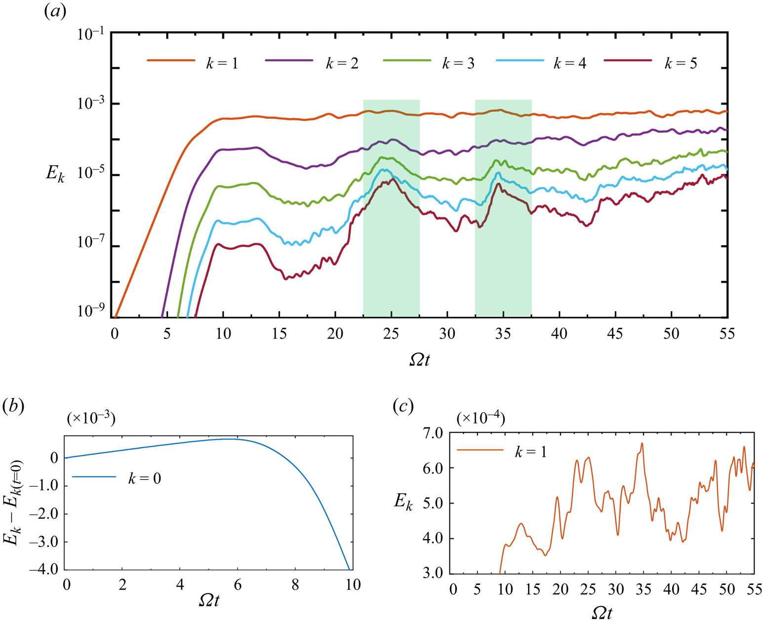
Figure 8. (a) Kinetic energies between Fourier modes  $k=1$ and
  $k=5$ at
  $Re=1.5\times 10^5$. (b) Kinetic energies in Fourier mode
  $k=0$ at
  $Re=1.5\times 10^5$. (c) Local magnification of the Fourier mode
  $k=1$.
From the described analysis, it can be inferred that, when  $\varOmega t > 40$ rad, higher radii consistently generated circular waves. These circular waves gradually created small-scale perturbation structures as they interacted with spiral waves during the downstream convective process, eventually resulting in localised turbulence at intermediate radii. However, at lower radii with lower Reynolds numbers and in the absence of spiral waves, the perturbations were solely caused by circular waves and did not give rise to localised turbulence.
To illustrate the location where localised turbulence occurred, figures 9(a) and 9(b), respectively, depict the non-dimensional axial velocity  $w/(\varOmega R)$ contour plots at
  $\varOmega t=50$ rad for the mean flow
  $k=0$, mode
  $k=1$ and mode
  $k=2$ at the meridional
  $(r, z)$ semiplane and plane at the
  $z/H=-0.98$, respectively. The mean flow contour plot reveals the presence of circular waves convecting downstream throughout the entire boundary layer. These circular waves interacted with the spiral waves in the boundary layer, leading to the generation of localised turbulence. Due to the strong perturbations already present in the current flow field, the
  $k=1$ mode only exhibited recognisable complete spiral waves at higher radii, while the spiral waves structure essentially disappears in the mid–lower-radius region. The perturbations of the mode
  $k=2$ mainly existed at the intermediate radius position, the radial location where localised turbulence was generated. As the Fourier mode varied (from 0 to 1 to 2), shown in figure 9(a), the radial scale depicted became smaller. Meanwhile, in figure 9(b), the azimuthal scale also became smaller. This phenomenon reinforces the previously mentioned correspondence between the radial small scale and the azimuthal small scale.
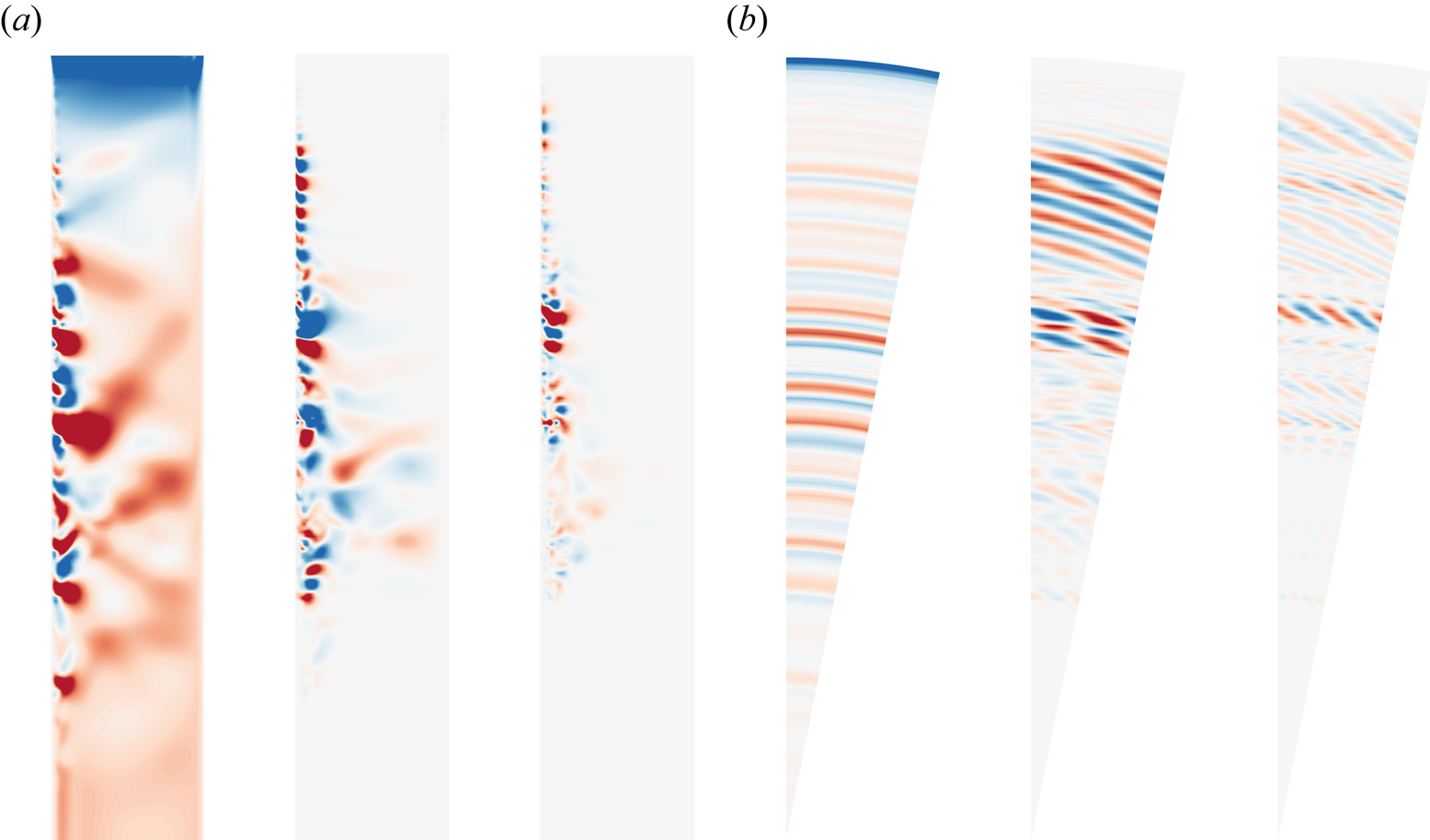
Figure 9. The visual representation of DNS at  $Re = 1.5 \times 10^5$: (a) meridional
  $(r, z)$ semiplane at
  $k=0, 1, 2$; (b) plane at
  $z/H=-0.98$ at
  $k=0, 1, 2$. The colour is consistent with figure 2(c), where the dimensionless axial velocity
  $w/(\varOmega R)$ ranges from
  $-$0.005 (blue) to 0.005 (red).
According to Jeong & Hussain (Reference Jeong and Hussain1995), the  $\lambda _2$ criterion can serve as a robust indicator for discerning vortex structures in the stationary-disk boundary layer. The contour plot shown in figure 10 illustrates the isosurface at
  $\lambda _2=-0.001$. When computing
  $\lambda _2$, the velocity and spatial scales were appropriately non-dimensionalised by
  $\varOmega H$ and
  $H$, respectively. The colour represents the axial velocity
  $w/\varOmega R$ on the vortex structures. Figures 10(a) and 10(b) each display the 3-D vortex structures from distinct viewpoints. The majority of the boundary was populated by chaotic vortex structures. The spiral wave structure in the higher-radius region interacted with the circular wave structure, convecting downstream and creating large-scale vortices accompanied by small-scale vortices, ultimately leading to the formation of localised turbulence. In these regions, the vortex structures exhibited uniformity in both radial and azimuthal scales. However, in the lower-radius region, where spiral waves were absent, only the circular wave structure existed.
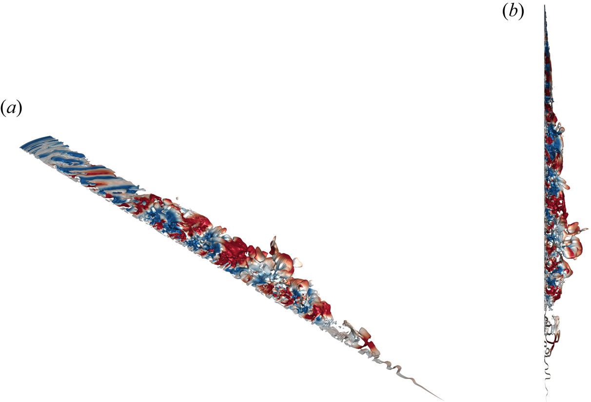
Figure 10. Vortical flow structures visualised by the iso-surface  $\lambda _2= -0.001$ coloured by
  $w/(\varOmega R)$ at
  $\varOmega t=50$ rad for
  $Re=1.5 \times 10^5$. The colour is consistent with figure 2(c), where the dimensionless axial velocity
  $w/(\varOmega R)$ ranges from
  $-$0.005 (blue) to 0.005 (red).
3.5. Turbulence transition pathway on the stationary-disk boundary layer
Based on the dynamic process of DNS, the pathway leading to the occurrence of localised turbulence in the boundary layer on the stationary-disk boundary layer could be summarised as follows.
After the linear energy growth of the perturbation eigenmode, nonlinear energy amplification caused the spiral waves to propagate upstream towards the high-radius region on the stationary-disk boundary layer. Subsequently, the spiral waves at the high-radius location on the stationary-disk boundary layer underwent nonlinear saturation. Following nonlinear saturation, the mean flow underwent significant changes owing to the influence of spiral waves, thereby inducing the appearance of circular waves. As an increasing number of circular waves propagated downstream from the higher-radius position of the boundary layer, they interact with the fully developed spiral waves, causing the formation of vertical structures that exist simultaneously at large and small scales, ultimately resulting in localised turbulence. At lower radial positions, the flow became relatively stable again due to the presence of only circular waves in the boundary layer.
Along the flow direction, from high to low radius, the process of laminar–transition–turbulent flow in the stationary-disk boundary layer can be qualitatively divided into four regions:
(i) In the outermost region, at a high radial distance from the centre, the boundary layer exhibits spiral waves indicative of type I instability.
(ii) Moving inward, an initial interaction between circular and spiral waves is observed. This interaction leads to mutual disturbances, which amplify the instability structures initially induced by the spiral waves.
(iii) Nearing the centre, the merging of larger-scale disturbances gives rise to localised turbulence. This turbulence is interspersed with high-frequency, small-scale perturbations and is typically found at mid-radii.
(iv) In the innermost region, at the lowest radial distance, the boundary layer is characterised by circular waves associated with type II instability.
4. Summary and conclusions
In the present study, the enigma surrounding the transition to turbulence in the stationary-disk boundary layer was addressed. The proposed approach seamlessly integrates global linear stability analysis and DNS to offer a fresh perspective on the matter. Notably, the current study's azimuthal wavenumber restriction, which only considers  $m=32$ and its harmonics, means that all other wavenumbers are excluded from the analysis. This limitation precludes the investigation of nonlinear interactions among all different azimuthal wavenumbers, which may play a significant role in the transition process. As a result, this study provides a possible transition mechanism of the stationary-disk boundary layer, considering only the nonlinear interactions of the azimuthal wavenumber
  $m=32$ and its harmonics. In future research, it is necessary to employ a full cavity model or experimental approaches to investigate the transition mechanism of the boundary layer under fully nonlinear interactions. The principal conclusions of the present study are as follows:
(i) Based on 452 data points spanning Reynolds numbers from
 $0.6 \times 10^5$ to $1.5 \times 10^5$, a contour plot was constructed to illustrate the relationship between the azimuthal wavenumber $m$ and the growth rate $\lambda _r$ of the perturbation eigenmode. Further, the critical Reynolds number ($Re_c$) at which global linear instability exists was determined to be $Re_c=51748$ when $m=32$.
(ii) For lower Reynolds numbers,
$Re=1.2 \times 10^5$, the DNS results reveal that the energy of the spiral mode initially increased linearly. With the emergence of nonlinear effects, the disturbance of the spiral waves propagated upstream to higher radial positions. Subsequently, circular waves of type II instability, generated due to mean flow distortion, occupied the entire lower-radius position. For higher Reynolds numbers, $Re=1.5 \times 10^5$, the linear and nonlinear processes were consistent with $Re=1.2 \times 10^5$. However, in this scenario, circular waves originate from higher radial positions and interfere with the spiral waves during their downstream development. This interference exacerbates the instability of the boundary layer, leading to the generation of localised turbulence(iii) Combining the 2-D base flow with the perturbation eigenmode at a specific azimuthal wavenumber, the initial flow for the 3-D DNS was derived. This approach facilitated the capture of the spiral instability of the flow without introducing additional perturbations. Subsequently, the interaction between type I and type II instabilities within the stationary-disk boundary layer triggered the emergence of localised turbulence in the rotor–stator cavity.


When investigating the transition to turbulence on the rotating-disk boundary layer, the flow generally underwent a process from low Reynolds numbers upstream to high Reynolds numbers downstream. As the disturbances developed and the local Reynolds numbers increased, whether due to convective instability or absolute instability, localised turbulence naturally appeared at a specific critical location. Further downstream, the development of turbulence became more vigorous. Therefore, research on the turbulence route on the stationary-disk boundary layer should not solely focus on the idea that turbulence appears first at high radii (Reynolds numbers). This approach can be misleading, as when turbulence appears at high radii, the mid- to low-radius regions of the entire boundary layer may already be chaotic with localised turbulence. This could explain why there is limited research on the study of turbulence pathways on the stationary-disk boundary layer.
However, the present study can serve as an initial exploration of the transition mechanism on the stationary-disk boundary layer. In future research, more rigorous discussions and analyses are required. Firstly, it is crucial to establish an appropriate reference base flow that can connect the present study with local stability analysis. Secondly, investigating whether the transition mechanism aligns with the findings of the current study in the presence of pulsatile or sustained disturbances would further enhance the credibility of the study. Finally, although there are challenges in obtaining the perturbation eigenmode from the present global linear stability analysis, using other methods, experiments or DNS can be employed to introduce circumferentially uniformly distributed roughness on the disk. This approach would force the generation of a specific azimuthal wavenumber for comparative analysis with the current study.
Acknowledgements
The authors extend their sincere gratitude to D. Fan, J. Liu, Z. Zhang and S. Liu for their valuable assistance and insightful discussions on numerical simulation. We would also like to thank the referees for their constructive comments on this paper.
Funding
The authors wish to acknowledge the financial support of the National Natural Science Foundation Outstanding Youth Foundation (grant no. 52122603), the National Science and Technology Major Project (J2019-III-0003-0046), Taishan Scholars Program and the cloud computing supported by the Beijing Super Cloud Computing Center.
Declaration of interest
The authors report no conflict of interest.


