


1. Introduction
Dual-robot system has high flexibility and efficiency, and they can complete some complex tasks that a single robot hard to finish [Reference Xiao, Zhang, Liao, Zhang, Ding and Jin1]. Because of these advantages, the dual-robot system has been widely used in many industrial scenes, such as loading, assembling, welding, and so on [Reference Yagiz, Hacioglu and Arslan2–Reference Xiong, Fu, Chen, Pan, Gao and Chen4]. However, the two robots in the dual-robot system share the same workspace, when the two robots cross to palletizing, they are prone to collide during the process of movement [Reference Yoon, Chung and Hwang5], which can hurt productivity and even cause serious production accidents [Reference Zhang, Zheng, Chen, Kong and Hamid6]. Therefore, it is necessary to realize the collision avoidance of the dual-robot system in an effective way. Many collision avoidance trajectory planning methods for the dual-robot system have been proposed in previous literatures. These usually can be divided into two sorts: kinematical-based method and intelligent optimization algorithm-based method.
Dual-robot trajectory planning based on kinematics is one of the main methods to realize collision avoidance. Kinematic collision avoidance trajectory planning is realized by modifying robot’s path, joint velocity, and acceleration. With the method of kinematic collision avoidance trajectory planning, Kang et al. [Reference Shin and Zheng7] gave a collision-free trajectory planning program for a dual-robot system by making one robot move along its path as fast as possible and delaying the other robot at the initial position. The two robots reached their final position without a collision. Chang et al. [Reference Chang, Chung and Lee8] proposed a collision map method, which can be used to describe collisions between two robots effectively. The minimum delaying time value of the robots was obtained by following the boundary contour of collision region on collision map. This method realizes the collision avoidance of dual-robot by delaying a short time. Ju et al. [Reference Ju, Liu and Hwang9] proposed a real-time velocity alteration strategy. In this approach, the two robots were set with low and high priority, respectively. The robot with low priority changed its speed by calculating the collision trend index to avoid the collision. The collision can also be avoided by locally changing the path of the robot. On the basis of the B-spline knot refinement and the local modification scheme, Chen et al. [Reference Chen and Li10] proposed an approach that only changes the local trajectory around collision area without changing the shape in the global way.
In aspect of the intelligent optimization algorithm-based method, Liang et al. [Reference Liang, Xu, Zhou, Li and Ye11] proposed a dual-robot collision-free motion planning strategy based on a dynamic neural network with physical constraints, which can successfully avoid collision. By taking this approach, the planning errors of 8-DOF modular robot and 14-DOF Baxter robot are reduced to 0 within 0.5 s and 0.3 s, respectively. Liu et al. [Reference Liu, Yu, Sheng and Zhang12] gave a 6-DOF dual-robot collision avoidance method based on the danger field. Meanwhile, a robust decentralized control strategy was proposed based on signal compensation and back-stepping. The result showed that the proposed scheme ensures that the space robotic system can automatically avoid self-collision and displays good robust performance. Su et al. [Reference Su and Xu13] combined the map search method with the time sampling method to search the optimal local path in each sampling time and synthesized all local paths into a complete path. The result showed that the proposal can successfully achieve collision avoidance of dual manipulators system while meeting the real-time requirements for multi-manipulator cooperate assembling scenarios. However, compared to the intelligent optimization algorithms used for the dual-robot system, there are more intelligent algorithms for the single robot obstacle avoidance trajectory planning, such as the C-space algorithm [Reference Zhao, Zhao, Duan, Gong and Bian14–Reference Masehian and Amin-Naseri16], grids algorithm [Reference Ferguson and Stentz17, Reference Duchon, Andrej, Martin, Peter, Martin, Tomas and Ladislav18], genetic algorithm [Reference Merchan-Cruz and Morris19–Reference Abu-Dakka, Valero, Suñer and Mata21], ant colony algorithm [Reference Yang, Qi, Miao, Sun and Li22], artificial network [Reference Xu, Zhou and Li23, Reference Ameer, Li and Luo24], and the APF method [Reference Fethi, Boumedyen and Mohamed25]. The application results of these methods in the dual-robot trajectory planning remained to be explored.
The artificial potential field (APF) algorithm is an obstacle avoidance algorithm [Reference Khatib26], which has been widely used in obstacle avoidance of a single robot because of its simplicity, practicability and good real-time performance. Compared to intelligent algorithms, it does not require too much computation or complex theoretical models. Wang et al. [Reference Wang, Zhu, Wang, He, He and Xu27] used the APF algorithm to plan the path of the 9-DOF redundant manipulator. By setting the angular velocity and angular acceleration of the robot in a limit range, the robot can maintain a safe distance from the obstacle. Anoush and Amirreza [Reference Anoush and Amirreza28] combined the APF method with randomized trees algorithm to plan the path of the robot. By this method, the robot can bypass the obstacles to reach the target point with the maximum position and direction errors are 0.01 m and 3°, respectively. Zhou et al. [Reference Zhou, Zhou, Yu, Zhang and Liu29] combined the APF method with cosine adaptive genetic algorithm, and the motion simulation analysis of 5-DOF pickup manipulator was carried out. This method realized the trajectory optimization of the manipulator in the obstacle environment and improved the pickup efficiency. Park et al. [Reference Park, Lee and Kim30] proposed a method combining numerical method based on Jacobian matrix and APF method to solve the real-time inverse kinematics and trajectory planning of redundant robots in unknown environment. This method simplified the solution of inverse kinematics, and through the motion planning experiment of 7-DOF robot, it was proved that this method can successfully avoid collision. These studies have shown that the APF algorithm has effective obstacle avoidance and navigation ability.
However, the traditional APF algorithm has been rarely used in collision avoidance trajectory planning of the dual-robot system. This is because it has the problems such as oscillation phenomenon in the target point and easy to fall into local minimum points [Reference Zhang, Zhu, Liu and Xu31]. To solve these problems of the traditional APF method, many modified APF methods are proposed, such as Xu et al. [Reference Xu, Zhou, Tan, Li, Fu and Peng32] proposed that when the robot falls into the local minimum, the robot was set to move along the direction of the potential surface of repulsive potential energy, so as to make the robot break away from the local minimum. Tang et al. [Reference Tang, Xu, Wang, Kang and Xie33] modified the potential field and force model of the APF method, reduced the amount of calculation of the algorithm, and avoided the problems of target unreachable and local minimum trap. Compared with the traditional APF method, the modified APF reduced the operation time by 54.89% and the total joint error by 45.41%. These studies show that appropriate modifications of the traditional APF method can reduce the impact of the shortcomings of the algorithm and improve the performance of the algorithm.
In this paper, a collision avoidance trajectory planning method for dual-robot systems based on a modified APF approach is proposed. The frame diagram of this study in a dual-robot palletizing field is shown in Fig. 1. Firstly, a collision detection model of the dual-robot system is established. And then, a modified APF algorithm was proposed. Finally, this paper studied the application of the collision avoidance trajectory planning strategy in a dual-robot palletizing field, and the performance of the proposed method is investigated by a trajectory planning simulation and experiment. This study will provide important guidance for the design of dual-robot collaborative operation trajectories that are collision avoidance and high-efficiency oriented.

Figure 1. The frame diagram of this study in a dual-robot palletizing field.
2. Dual-robot kinematic model and collision detecting
In a dual-robot system, two robots operate within the same workspace and are at risk of colliding with each other. To address this issue, kinematic analysis was conducted to determine an effective collision detection method between the two robots.
2.1. Kinematic modeling of the dual-robot system
Second, the simplified structure of a dual-robot system is shown in Fig. 2. There are two 6-DOF multi-joint robots, named R1 and R2, in the dual-robot system. The two robots are horizontally arranged, where O1 is the base position of the robot R1, Ji (i = 1,2…,6) represents the joint of the robot. O2 is the base position of the robot R2, Jiʹ(i = 1, 2, …, 6) represents the joint of the robot R2. L1 represents the distance between the base positions of two robots. The sum of the working radii of the two robots is larger than L1, when the two robots palletize together, there might have been a collision between the two robots.

Figure 2. Simplified structure of the dual-robot.
The kinematics model of the robot was established by the modified D-H method [Reference Liu, Xiao, Tong, Tao, Xu, Jiang, Chen, Cao and Sun34]. According to the modified D-H method, the coordinate relationship between two adjacent links of the robot is shown in Eq. (1).
 \begin{equation}{}^{{i}-1\!\!}{}_{{i}}{{T}}{}=\left[\begin{array}{c@{\quad}c@{\quad}c@{\quad}c} c{\theta }_{{i}} & {-}{s}{\theta }_{{i}} & 0 & {p}_{{i}{-}1}\\[5pt] {s}{\theta }_{{i}}{c}{\alpha }_{{i}{-}1} & {c}{\theta }_{{i}}{c}{\alpha }_{{i}{-}1} & {-}{s}{\alpha }_{{i}{-}1} & {-}{d}_{{i}}{s}{\alpha }_{{i}{-}1} \\[5pt] {s}{\theta }_{{i}}{s}{\alpha }_{{i}{-}1} & {c}{\theta }_{{i}}{s}{\alpha }_{{i}{-}1} & c{\alpha }_{{i}{-}1} & {d}_{{i}}{c}{\alpha }_{{i}{-}1}\\[5pt] 0 & 0 & 0 & 1 \end{array}\right]\end{equation}
where α i is twist angle, p i is link length, d i is link offset, θ i is joint angle, i = 1, 2, …, 6, sθ i =sinθ i , cθ i =cosθ i . Since the six joints of the robot are rotating joints, the joint angle θ i is the only variable in the D-H parameters of the robot.
The forward kinematics equation of the robot is shown in Eq. (2), and it was obtained by multiplying the coordinate transformation matrices.
 \begin{equation}{}_{6}^{0}{{T}}{}={}_{1}^{0}{{T}}{}_{2}^{1}{{T}}{}_{3}^{2}{{T}}{}_{4}^{3}{{T}}{}_{5}^{4}{{T}}{}_{6}^{5}{{T}}{}\end{equation}
2.2. Collision criterion of the two robots
The master/slave control strategy is suitable for the situation where the velocity of the robot is moderate and the operating object is not easy to distort [Reference Kosuge, Ishikawa, Furuta and Sakai35]. The principle of this strategy is to satisfy the task requirements of the master robot first and to make the trajectory of a slave robot based on the trajectory of the master robot. The master/slave control strategy was used in the dual-robot system, the robots R1 and R2 are set as the master robot and the slave robot, respectively. When a collision between the two robots is detected, the trajectory of the slave robot will be modified. Therefore, robot R1 can be regarded as a dynamic obstacle of robot R2. The distances between the end effector of robot R2 and the joints, links, end effector of robot R1 are taken as the main judgment parameters of collision.
To analyze the collision problem, the dual-robot system was simplified into a geometric model. The end effector of the two robots was regarded as a spherical body with a radius of r a . The joint of the two robots was regarded as a spherical body with a radius of r b . The link of the two robots was regarded as a cylindrical body with a length of l b , and the radius of the cylinder is r c . The positional relationships between the geometries are shown in Fig. 3. The distances between the end effector of robot R2 and the joints of robot R1 are [d 1,…,d i ] (i = 1, 2, …, 6). The distances between the end effector of robot R2 and the links of robot R1 are [d 1, …, d j ] (j = 1, 2, …, 6). The distance between the end effector of R2 and the end effector of robot R1 is d k . The two robots collide when the following criteria in Eq. (3) are met.
 \begin{align} \begin{cases} \begin{array}{c} \min \left[{d}_{1},\ldots,{d}_{{i}}\right]\gt {r}_{{a}}{+}{r}_{{b}}={d}_{{s}1},{i}=1,2,\ldots,6\\[5pt] \mathrm{or} \end{array}\\[5pt] \begin{array}{c} \min \left[{d}_{1}{,}{\ldots }{,}{d}_{{j}}\right]{\gt }{r}_{{a}}{+}{r}_{{c}}={d}_{{s}2},{j}=1,2,\ldots,6\\[5pt] \mathrm{or} \end{array}\\[5pt] \quad\qquad\qquad {d}_{{k}}\gt {r}_{{a}}+{r}_{{d}}={d}_{{s}3} \end{cases}\end{align}
where d s1, d s2, d s3 are the minimum safe distances from the end effector of robot R2 to joints, links, and end effector of robot R1, respectively.

Figure 3. The positional relationships between geometries. (a) R1’s joints and R2’s end effector. (b) R1’s links and R2’s end effector. (c) R1’s end effector and R2’s end effector.
3. The TAPF algorithm and a modified APF algorithm
The traditional APF algorithm (TAPF) is a local trajectory planning method by establishing virtual APFs in the motion space of the robot [Reference Khatib36]. The APF is composed of attractive field and repulsive fields. The attractive field is set at the target point, and the repulsive fields are set at the obstacles. The robot avoids obstacles under the action of repulsive fields and reaches the target point under the action of the attractive field. The function of the traditional attractive potential field is shown in Eq. (4).
 \begin{equation}{U}_{\mathrm{att}}=\frac{1}{2}{K}_{\mathrm{att}}{\rho }({q}{,}{{q}_{{g}}})^{2}\end{equation}
where K
att is the attractive coefficient. $\rho$
(q, q
g
) is a vector, its value is equal to the Euclidean distance from the current position of the robot q to the target point q
g
, and its direction is along a straight line from the position of the robot to the target point. The function of the virtual attractive potential force is shown in Eq. (5).
$\rho$
(q, q
g
) is a vector, its value is equal to the Euclidean distance from the current position of the robot q to the target point q
g
, and its direction is along a straight line from the position of the robot to the target point. The function of the virtual attractive potential force is shown in Eq. (5).
 \begin{equation}{F}_{\mathrm{att}}=-\nabla {U}_{\mathrm{att}}={K}_{\mathrm{att}}{\rho }({q},{q}_{{g}})\end{equation}
The repulsive potential fields are set at the joints of robot R1. The function of the repulsive potential field is shown in Eq. (6).
 \begin{equation}{U}_{\mathrm{rep}{\_ }{i}}=\left\{\begin{array}{ll} \dfrac{1}{2}{K}_{\mathrm{rep}}\left(\dfrac{1}{{\rho }({q},{q}_{{i}})}-\dfrac{1}{{d}_{{i}}}\right)^{2}, & {d}_{{i}}\leq {r}_{{s}}\\[12pt] \mathrm{0} & \!\!\!,{d}_{{i}}\gt {r}_{{s}} \end{array}\right.\end{equation}
where K
rep is the repulsive coefficient. $\rho$
(q, q
o
) is a vector, its value is equal to the Euclidean distance from the current position of the robot q to the obstacle q
o
, and its direction is along a straight line from the position of the robot to the obstacle. d
i
is the distance between the robot and joint of robot R1 (i = 1, 2, …, 6), r
s
is the critical action distance of the repulsive potential field.
$\rho$
(q, q
o
) is a vector, its value is equal to the Euclidean distance from the current position of the robot q to the obstacle q
o
, and its direction is along a straight line from the position of the robot to the obstacle. d
i
is the distance between the robot and joint of robot R1 (i = 1, 2, …, 6), r
s
is the critical action distance of the repulsive potential field.
The function of the virtual repulsive force is shown in Eq. (7).
 \begin{equation}{F}_{\mathrm{rep}{\_ }{i}}=-\nabla {U}_{\mathrm{rep}{\_ }{i}}=\left\{\begin{array}{ll} {K}_{\mathrm{rep}}\left(\dfrac{1}{{\rho }\left({q},{q}_{{i}}\right)}-\dfrac{1}{{d}_{{i}}}\right)\dfrac{1}{{\rho }^{2}\left({q},{q}_{{i}}\right)}\nabla {\rho} \left({q},{q}_{{i}}\right),& {d}_{{i}}\leq {r}_{{s}}\\[12pt] \mathrm{0}& \!\!\!, {d}_{{i}}\gt {r}_{{s}} \end{array}\right.\end{equation}
The total potential field is the sum of the attractive potential field and all repulsive potential fields; it is as presented in Eq. (8).
 \begin{equation}{U}={U}_{\mathrm{att}}+\sum _{{i}=1}^{{n}}{U}_{\mathrm{rep}{\_ }{i}}\end{equation}
where U is the total potential field, n is the number of robot joints.
The resultant force on the robot is shown in Eq. (9).
 \begin{equation}{F} =-\nabla {U}={F}_{\mathrm{att}}{+}\sum _{{i}=1}^{{n}}{F}_{\mathrm{rep}{\_ }{i}}\end{equation}
Then, the joint acceleration of the robot can be obtained by Eqs. (10)–(12).
 \begin{equation}{M}={{J}_{{F}}}^{\mathrm{T}}({\theta }_{1},{\theta }_{2},\ldots,{\theta }_{6}){F}\end{equation}
 \begin{equation}{J}_{{F}}= \left[\begin{array}{c@{\quad}c@{\quad}c@{\quad}c@{\quad}c@{\quad}c} \dfrac{\partial x_{1}}{\partial \theta _{1}} & \dfrac{\partial x_{1}}{\partial \theta _{{2}}} & \dfrac{\partial x_{1}}{\partial \theta _{{3}}} & \dfrac{\partial x_{1}}{\partial \theta _{{4}}} & \dfrac{\partial x_{1}}{\partial \theta _{{5}}} & \dfrac{\partial x_{1}}{\partial \theta _{6}}\\[12pt] \dfrac{\partial x_{{2}}}{\partial \theta _{1}} & \dfrac{\partial x_{{2}}}{\partial \theta _{{2}}} & \dfrac{\partial x_{{2}}}{\partial \theta _{{3}}} & \dfrac{\partial x_{{2}}}{\partial \theta _{{4}}} & \dfrac{\partial x_{{2}}}{\partial \theta _{{5}}} & \dfrac{\partial x_{{2}}}{\partial \theta _{{6}}}\\[12pt] \dfrac{\partial x_{{3}}}{\partial \theta _{1}} & \dfrac{\partial x_{{3}}}{\partial \theta _{{2}}} & \dfrac{\partial x_{{3}}}{\partial \theta _{{3}}} & \dfrac{\partial x_{{3}}}{\partial \theta _{{4}}} & \dfrac{\partial x_{{3}}}{\partial \theta _{{5}}} & \dfrac{\partial x_{{3}}}{\partial \theta _{{6}}}\\[12pt] \dfrac{\partial x_{{4}}}{\partial \theta _{1}} & \dfrac{\partial x_{{4}}}{\partial \theta _{{2}}} & \dfrac{\partial x_{{4}}}{\partial \theta _{{3}}} & \dfrac{\partial x_{{4}}}{\partial \theta _{{4}}} & \dfrac{\partial x_{{4}}}{\partial \theta _{{5}}} & \dfrac{\partial x_{{4}}}{\partial \theta _{{6}}}\\[12pt] \dfrac{\partial x_{{5}}}{\partial \theta _{1}} & \dfrac{\partial x_{{5}}}{\partial \theta _{{2}}} & \dfrac{\partial x_{{5}}}{\partial \theta _{{3}}} & \dfrac{\partial x_{{5}}}{\partial \theta _{{4}}} & \dfrac{\partial x_{{5}}}{\partial \theta _{{5}}} & \dfrac{\partial x_{{5}}}{\partial \theta _{{6}}}\\[12pt] \dfrac{\partial x_{6}}{\partial \theta _{1}} & \dfrac{\partial x_{{6}}}{\partial \theta _{{2}}} & \dfrac{\partial x_{{6}}}{\partial \theta _{{3}}} & \dfrac{\partial x_{{6}}}{\partial \theta _{{4}}} & \dfrac{\partial x_{{6}}}{\partial \theta _{{5}}} & \dfrac{\partial x_{6}}{\partial \theta _{6}} \end{array}\right] \end{equation}
 \begin{equation}\ddot{{\theta }}={M}/{B}_{{J}}\end{equation}
where M is the joint torque, J
F
is the Jacobian matrix, $\ddot{{\theta }}$
is the joint acceleration of the robot, B
J
is the inertia of the robot joint.
$\ddot{{\theta }}$
is the joint acceleration of the robot, B
J
is the inertia of the robot joint.
However, there are two defects of the APF algorithm, which affect its application in dual-robot trajectory planning. The attractive potential force of the traditional APF algorithm is related to the joint acceleration of the robot. Under the action of potential force, when the robot moves to the target point, the joint acceleration is reduced to 0 m/s2, while the joint speed of the robot is not reduced to 0 m/s. This will cause the robot to oscillate under the action of potential field force instead of stopping at the target point [Reference Yang, Wu, Zhou, Lv, Liu, Zhang, Hou and Wang37]. And in the traditional APF algorithm, the attractive potential force is proportional to the distance between the robot and the target point. When the robot is far from the target point, the attractive force will be large, which may cause the two robots to collide.
To solve the defects of the traditional APF algorithm, two improvements are made to the traditional APF algorithm in the present study:
1) To solve the problem of excessive attractive potential force, r q was defined as a threshold distance for attractive potential filed. When the distance between the robot and the target point is less than or equal to r q , the attractive potential force is proportional to the distance. When the distance between the robot and the target point is greater than critical action distance r q , the attractive force is set to be U k , the value of U k is equal to the value of U att when the distance from the robot end effector to the target point is r q . The functions of the modified attractive potential field and virtual attractive potential force are shown in Eqs. (13) and (14).
 \begin{equation}{U}_{\mathrm{att}}=\left\{\begin{array}{ll} \dfrac{1}{2}{K}_{\mathrm{att}}{\rho }({q}{,}{{q}_{{g}}})^{2},& {d}_{{q}}\leq {r}_{{q}}\\[12pt] {U}_{{k}}&\!\!\!,{d}_{{q}}\gt {r}_{{q}} \end{array}\right.\end{equation}
 \begin{equation}{F}_{\mathrm{att}}=-\nabla {U}_{\mathrm{att}}=\left\{\begin{array}{ll} {K}_{\mathrm{att}}{\rho} (\mathrm{q},{q}_{{g}}),& {d}_{{q}}\leq {r}_{{q}}\\[5pt] {F}_{{k}}&\!\!\!, {d}_{{q}}\gt {r}_{{q}} \end{array}\right.\end{equation}
where d q is the distance between the robot and the target point, F k is the value of F att when the distance from the robot end effector to the target point is r q .
2) In order to solve the problem of oscillation at the target point, the virtual force field was directly transformed into joint velocity rather than joint acceleration. Thus, the joint velocity of the robot can be obtained by Eqs. (10)–(11) and Eq. (15).
 \begin{equation}\dot{{\theta }}=K_{v}{M}/{B}_{{J}}\end{equation}
where $\dot{{\theta }}$
is the joint velocity of the robot and K
v
is the joint velocity coefficient.
$\dot{{\theta }}$
is the joint velocity of the robot and K
v
is the joint velocity coefficient.
4. Application of dual-robot system in palletizing
4.1. Working condition of the dual-robot system
As an example of research, a bagged cement loading system using dual robots is analyzed. The system is mainly composed of a dual-robot system, mechanical grippers, vehicle contour scanning system, bagged cement conveyor, dust collector, gantry truss walking mechanism, and control system. The dual-robot system consists of two KR240 R3100 K ultra-A robots, which have 6-DOF. The loading system and key parameters of the robot are given in Fig. 4. The schematic diagram of the robot geometric parameters is shown in Fig. 5. The robot’s D-H parameters were calculated using Eqs. (1) and (2), and the results are listed in Table 1.

Figure 4. The loading system and key parameters of the robot.

Figure 5. The schematic diagram of the robot geometric parameters.
Table 1. D-H parameters of KUKA KR240 R3100 K ultra-A robot.

Figure 6 shows the mechanical gripper of the robot and the size of the palletizing bag. The gripper can grab two bags at a time, and the size of bag is 0.64 m × 0.5 m. According to the Section 2.2, the mechanical gripper can be regarded as a spherical body with a radius of 0.64 m. The minimum safe distance d s3 between two robots was set to be 1.28 m. In order to prevent the collision between two robots, the critical action distance of the repulsive potential field r s was set to 1.92 m, with a margin of 50%. The minimum safe distances d s1 and d s2 were all set to be 0.8 m.

Figure 6. The mechanical gripper of the robot and size of the palletizing bag.
4.2. Dual-robot collision avoidance trajectory planning
For robot R1 in the dual-robot system, its palletizing trajectory can be defined by using the “point-to-point” method. As shown in Fig. 7, the palletizing process was divided into three steps with four necessary passing locations (or points), where P1 is the initial location. P2 and P3 are two intermediate locations. P4 is the target location. The three steps are as follows.

Figure 7. The schematic diagram of the robot’s trajectory.
Step 1. The robot grabs the bags at point P1 and then translates upward to reach the intermediate point P2.
Step 2. The robot moves from intermediate point P2 to intermediate point P3. The trajectory from P2 to P3 can be fitted by the cubic polynomial curve. The cubic polynomial interpolation equation is shown in Eq. (16).
 \begin{equation}\begin{cases} {\unicode[Arial]{x03B8}} \left({t}\right)={a}_{0}+{a}_{1}\mathrm{t}+{a}_{2}{t}^{2}+{a}_{3}{t}^{3}\\[5pt] \dot{{\theta }}\left({t}\right)={a}_{1}+\mathrm{2}{a}_{2}\mathrm{t}+3{a}_{3}{t}^{2} \\[5pt] \ddot{{\theta }}\left({t}\right)=\mathrm{2}{a}_{2}+\mathrm{6}{a}_{3}\mathrm{t} \end{cases}\end{equation}
where θ(t), $\dot{{\theta }}(\mathrm{t})$
,
$\dot{{\theta }}(\mathrm{t})$
, $\ddot{{\theta }}({t})$
represent joint angle, joint velocity, and joint acceleration, respectively. a
0, a
1, a
2, a
3 are the polynomial interpolation coefficients.
$\ddot{{\theta }}({t})$
represent joint angle, joint velocity, and joint acceleration, respectively. a
0, a
1, a
2, a
3 are the polynomial interpolation coefficients.
Step 3. The robot translates downward from intermediate point P3 to target point P4.
The procedure of collision avoidance trajectory planning method is shown in Fig. 8. First, the initial points and the target points of the two robots are determined, and the initial trajectories for the two robots were generated. Second, the distances between robot R1 and robot R2 at each moment in the trajectories are calculated. When the distances (d i , d j , d k ) are less than the 1.5 times of the minimum safe distances (d s1, d s2, d s3), the two robots are considered to have collision risk. Third, when a collision risk between the two robots is detected, the modified APF algorithm starts to work. The virtual attractive field and repulsive fields are set in the workspace of the dual-robot system to modify the trajectory of the robot R2. And robot R2 will avoid away from robot R1 under the action of repulsive potential fields. After robot R1 completes its palletizing task and leaves, robot R2 will reach the target point under the action of the attractive potential field. The schematic diagram of the modified trajectory of robot R2 is shown in Fig. 9.

Figure 8. The procedure of collision avoidance trajectory planning.
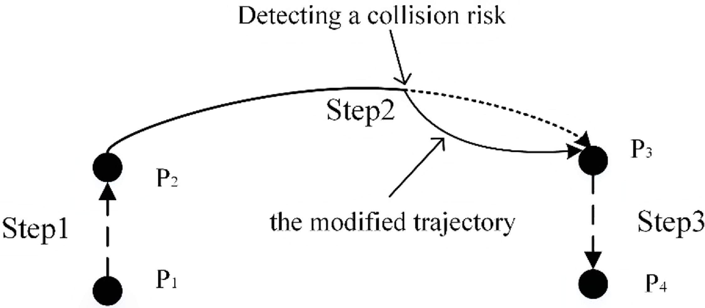
Figure 9. The schematic diagram of the robot R2’s modified trajectory.
4.3. Verification of trajectory planning method
The collision avoidance performance of the collision avoidance algorithm was verified through a trajectory planning simulation method. The three-dimensional geometric model of the robot was established using SolidWorks software, and the kinematic model of the dual-robot system was established according to the D-H parameters of the robot. Through the SW2URDF plug-in, the three-dimensional model of the robot was transformed into the URDF file. Then, the URDF file of the dual-robot system was imported into MATLAB software, and its trajectory planning simulation can be carried out using the Robotics System Toolbox. The experiment has been conducted under the working conditions given in Section 4.1.
The reachable positions of the two robots are shown in Fig. 10, which are represented by scattered points. The blue points represent the reachable positions of the robot R1, and the red points represent the reachable positions of the robot R2. It can be seen that the workspace of the two robots has obvious overlapping region.

Figure 10. Three-dimensional model of the dual-robot in MATLAB.
The collision avoidance simulation of the dual-robot system was conducted using two different methods: with and without collision avoidance. In this simulation, the two robots were placed 2.25 m apart along the Y-axis, with their base coordinates at [0, 0, 0] and [0, 2.25, 0], respectively. Robot R1 started at initial point [1.5, −1.2, −0.5] and aimed to reach target point [2, 0.5, −1], while robot R2 began at initial point [1.5, 3.45, −0.5] and aimed for target point [2, 1, −1]. These target points are marked by red and blue dots in Fig. 10. The attractive coefficient K att was set to 1, while the repulsive coefficient K rep was set to 3.
Figure 11 shows the trajectories of the two robots without applicating the collision avoidance algorithm. The distances between the end effector of robot R1 and the joints of robot R2 in the working process are shown in Fig. 12. It can be seen from Fig. 11 that, in the 3.75–6.35 s time period, the distances between the end effector of robot R2 and J4, J5, J6 of robot R1 are less than the minimum safe distance d s1, which means that there is a collision between the two robots.

Figure 11. The trajectory of the dual-robot system without collision avoidance.

Figure 12. The distances from end effector of R2 to joints of R1 without the collision avoidance algorithm.
The modified APF collision avoidance algorithm was applied to the trajectory planning of the dual-robot system, resulting in the trajectories shown in Fig. 13. Figure 13a and b display the initial trajectories of the two robots when no collision risk was detected. However, upon detecting a potential collision, the trajectory of robot R2 was adjusted using the proposed APF algorithm, as illustrated in Fig. 13c. The modified trajectory of robot R2 is depicted in Fig. 13d, showing its successful arrival at the target point under the influence of the virtual attractive potential field. Meanwhile, robot R1 moves towards its target point in both Fig. 13a and Fig. 13b, and returns to its starting position in Fig. 13c and Fig. 13d.

Figure 13. The trajectory of the dual-robot system with the modified APF algorithm.
Figures 14 and 15 give the distances from the end effector of robot R2 to the joints and links of robot R1. It can be found that the collision risk was detected at 2.9 s, and the end effector of robot R2 generated a partial velocity away from robot R1 from this moment on. After 4.8 s, the distance between robot R2 and R1 is no longer reduced. During the whole process, the distances from robot R2 to the joints and links of robot R1 are greater than the minimum safe distance d s1 and d s2, respectively. This result indicates that the proposed APF collision avoidance algorithm can effectively avoid the collision between the two robots.

Figure 14. The distances from the end effector of R2 to joints of R1 with the proposed APF algorithm.

Figure 15. The distances from end effector of R2 to links of R1 with the proposed APF algorithm.
The rapidly exploring random tree (RRT) algorithm is a trajectory search method of incremental sampling. It is often used for static and dynamic obstacle avoidance of robots [Reference Ryo and Takeshi38, Reference Kang, Lim, Choi, Jang and Jung39]. In this simulation experiment, the RRT algorithm and the traditional APF method were used as comparison algorithms to verify the effectiveness of the algorithm proposed in this paper. The random sampling probability is set to 0.5, the rapidly exploring random tree has a probability of 0.5 to directly advance the sampling end point, and a probability of 0.5 to advance in any direction within the space. To match the motion speed of the robot, the growth step was set to 0.025m.
Simulation results show that the modified APF algorithm took 8.2 s to obtain the modified trajectory of robot R2, while it was 11.1 s for RRT and 215.3 s for the traditional APF algorithm. In addition, the modified APF algorithm’s convergence time is 0.9 s, which is 14.2% faster than that of the traditional APF algorithm. The distances from the end effector of R2 to the end effector of R1 during the movement of the two robots are given in Fig. 16. As shown in the figure, the trajectory generated by RRT has obvious oscillation phenomenon in the process of obstacle avoidance, while the trajectory is smooth generated by the modified APF method. In addition, the minimum distance between the end effectors of two robots with the traditional APF method is smaller than the minimum safe distance (1.28 m). The safety factor SA is utilized to assess the safety of robot trajectories, which is calculated as the ratio of the shortest distance between end effectors to the minimum safe distance. The safety factors for robot operation obtained through the modified APF, traditional APF, and RRT method are presented in Table 2. It is evident that the robot trajectory safety factor obtained through the modified APF method is 11% and 4% higher than those obtained by the traditional APF and RRT method, respectively. The results indicated that the improved APF algorithm can ensure the distance between the end effectors of the two robots is greater than the minimum safe distance, and the experimental results confirmed this conclusion. Meanwhile, the oscillation phenomenon induced by the traditional APF algorithm and RRT was avoided when using the modified APF algorithm.

Figure 16. The distances from end effector of R2 to end effector of R1.
4.4. Experiment validation
As described in Section 4.1, the dual-robot system was mounted on a gantry with a height of 5.13 m. The robots have a repetitive positioning accuracy within ±1 mm and a maximum working radius greater than 2.5 m. The platform at the top of the gantry measures 5.90 m in length and 2.72 m in width. A conveyor belt is installed below the platform to transport bags to the grab position. The two robots used in this system are KUKA KR270 R3100 ultra K models, controlled by KUKA KR C4 and programmed using KUKA smartPAD. The dual-robot collision avoidance experiment platform is depicted in Fig. 17.
The complete experimental process is as follows:
Step 1: Determine the position and attitude of the teaching point through the teaching device and input the position transition radius, attitude transition radius and other given trajectory parameters at the same time;
Step 2: The control module reads the position and attitude of the input teaching point, position transition radius, attitude transition radius, and other given trajectory parameters;
Step 3: According to the read parameters, the control module obtains the functional relationship between the position trajectory length and time at the end effector of the robot and the functional relationship between the angular displacement length of the attitude trajectory and time through the compiled end trajectory planning algorithm program of the robot;
Step 4: The control module performs isochronous interpolation and calculates the displacement and angular displacement corresponding to the interpolation time according to the functional relationship between the position trajectory length and the angular displacement length of the attitude trajectory and time in each interpolation cycle;
Step 5: Calculate the position and attitude of the corresponding interpolation point at the interpolation time according to the length of the position trajectory and the angular displacement length of the attitude trajectory corresponding to the interpolation time through the interpolation algorithm of the position trajectory and the interpolation algorithm of the attitude trajectory;
Step 6: According to the position and posture of the interpolation point, the joint angles corresponding to the interpolation point are obtained through the robot kinematics model and inverse kinematics program;
Step 7: Send the angles of each joint to the servo driver. The servo driver drives the servo motors of the six joint axes of the six-axis robot to rotate according to the input joint angle signal.
The experiment demonstrates the working process of the loading system, two robots respectively grab 100 kg bags of cement for palletizing work. When the collision avoidance algorithm detects a collision risk, the slave robot starts to change its trajectory away from the master robot, while the master robot keeps its own trajectory unchanged, so as to complete the palletizing work without collision.
Table II. Robot trajectory safety factor values obtained through the modified APF, traditional APF, and RRT method.


Figure 17. Dual-robot collision avoidance experiment.
The experimental results show that the proposed collision avoidance algorithm can meet the safety work requirements of the dual-robot system. The two robots can avoid collisions during their work process. The dual-robot system adopts the proposed trajectory planning method, which can achieve the goal of loading 2000 bags of cement per hour.
5. Conclusions
To solve the collision problem that may occur during the working process of the dual-robot system, a collision avoidance trajectory planning method was proposed in the present study. The main conclusions were drawn as follows.
1. A dual-robot collision detection model was established. By which the distance between the two robots can be calculated to determine whether there is a collision between the two robots.
2. A collision avoidance trajectory planning method was proposed on the basis of a modified APF algorithm. By using the proposed APF algorithm, the problems of excessive attractive potential force and oscillation at the target point can be avoided.
3. It is proved that the proposed algorithm can be successfully applied in the field of dual-robot palletizing through simulation and experiment. The solution speed and convergence speed of the modified APF method are faster than that of the traditional APF algorithm. And the oscillation phenomenon rapidly-exploring random tree algorithm was solved by the modified APF algorithm.
The proposed algorithm is well-suited for the off-line design of initial trajectories for dual robots, but its primary limitation lies in its inability to handle real-time obstacle avoidance scenarios. Furthermore, we are confident that the proposed method can also be applied to complex environments. Nevertheless, due to limitations in our experimental setup, we have been unable to create a more intricate experimental scenario at present. In future research, we intend to explore more complex experimental subjects and provide a more comprehensive discussion on the benefits of the proposed approach.
Acknowledgements
The authors would like to express their thanks to Qirui He, who participated in the layout of the format
Author contributions
All authors contributed to the study conception and design. Methodology was designed by Dong Yang and Junkang Dai. Simulation was developed by Li Dong. The first draft of the manuscript was written by Dong Li. All authors commented on the manuscript. All authors read and approved the final manuscript.
Financial support
This work was financially supported by the Key Research and Development Program of Anhui Province (Grant No. 202004a05020059), and the Anhui Graduate Scientific Research Project (Grant No. YJS20210011).
Competing interests
The authors declare no competing interests.
Ethical approval
None.


