


1. Introduction
The accuracy of large-scale climate and ocean models depends on the parametrization of turbulent fluxes. Turbulent mixing events are often modelled using idealized shear instabilities in stratified flows. Shear instability has been observed in the stably stratified nocturnal atmospheric boundary layer (Newsom & Banta Reference Newsom and Banta2003; Smyth, Mayor & Lian Reference Smyth, Mayor and Lian2023) as well as at higher elevations (Fritts et al. Reference Fritts2023). Shear instability has also been observed in a variety of oceanic contexts, including equatorial undercurrents (Moum, Nash & Smyth Reference Moum, Nash and Smyth2011), flows over sills (Van Haren et al. Reference Van Haren, Gostiaux, Morozov and Tarakanov2014; Chang et al. Reference Chang2022), estuarine shear zones (Geyer et al. Reference Geyer, Lavery, Scully and Trowbridge2010; Holleman, Geyer & Ralston Reference Holleman, Geyer and Ralston2016; Tu et al. Reference Tu, Fan, Liu and Smyth2022), and the strongly stratified transition layer within the ocean surface boundary layer (Kaminski et al. Reference Kaminski, D'Asaro, Shcherbina and Harcourt2021).
Previous theoretical research on shear instabilities has assumed a single, isolated stratified shear layer (e.g. Caulfield & Peltier Reference Caulfield and Peltier2000; Mashayek & Peltier Reference Mashayek and Peltier2013; Salehipour & Peltier Reference Salehipour and Peltier2015; Kaminski & Smyth Reference Kaminski and Smyth2019; Lewin & Caulfield Reference Lewin and Caulfield2021; Liu, Kaminski & Smyth Reference Liu, Kaminski and Smyth2022, Reference Liu, Kaminski and Smyth2023), neglecting the potential influence of nearby flow structures. Our goal here is to relax the assumption of a single, isolated shear layer. As a starting point, we examine a pair of shear layers, varying the distance between them and analysing the resulting changes in the route to turbulence and in the resulting mixing.
This is the third in a sequence of three studies using ensembles of direct numerical simulations with small, random variations in the initial state. Liu et al. (Reference Liu, Kaminski and Smyth2022) (hereafter L22) showed that even a slight change in the initial perturbation can lead to significant variations in turbulence timing and strength due to interactions between the primary Kelvin–Helmholtz (KH), subharmonic, and three-dimensional (3-D) secondary instabilities. This resulted in differences of up to a factor of four in the maximum turbulent kinetic energy, and a factor of two in the potential energy gain due to mixing. Liu et al. (Reference Liu, Kaminski and Smyth2023) (hereafter L23) studied the effects of boundary proximity on KH instability. Boundary effects have a pronounced effect on the dynamics of KH instability, influencing its growth, secondary instability, and the resulting turbulent mixing. Notably, the cumulative mixing efficiency vanishes as the shear layer approaches a solid boundary. As in L22, these results were sensitive to small changes in the initial conditions, emphasizing the need to compare ensemble-averaged statistics.
Our work is motivated in part by observations of multiple stratified shear layers in geophysical fluids at consecutive depths, sometimes in close proximity to each other (Desaubies & Smith Reference Desaubies and Smith1982; Alford & Pinkel Reference Alford and Pinkel2000). Fritts et al. (Reference Fritts, Bizon, Werne and Meyer2003) showed layered structures in the atmosphere due to shear instability and gravity-wave breaking. Recent work on stratified shear flows reveals spontaneous organization into layers of quiescent, strongly stratified fluid and strongly turbulent, weakly stratified fluid (Woods Reference Woods1968; Caulfield Reference Caulfield2021). We therefore wonder about conditions under which instabilities of nearby shear layers could interact, and with what effect on instability, turbulence and mixing.
We find that as the separation distance between the two layers decreases to (approximately) the layer thickness, instability is suppressed. We also show that the presence of a neighbouring shear layer can excite one of two novel forms of instability, one stationary and one oscillatory. This distinction has profound effects on the transition to turbulence and the resulting mixing, including an abrupt change in mixing efficiency, even when the difference in initial states is small.
In § 2 we describe the set-up for our numerical simulations and the choice of the initial parameter values, as well as the diagnostic tools required for the analysis of 3-D energetics and mixing. We then describe the effects of neighbouring shear instability on the linear stability characteristics in § 3, and introduce the stationary and oscillatory modes of instability. In § 4, we analyse the perturbation kinetic energy budget to explain how a neighbouring shear instability could alter the route to turbulence. In § 5, we describe the neighbouring effects on the irreversible mixing and mixing efficiency. Conclusions are summarized in § 6, and possible directions for future research are discussed in § 7.
2. Methodology
2.1. The mathematical model
We begin by considering a stably stratified parallel shear flow,
 \begin{equation} U^{*}(z)=U^{*}_{0}\left[\tanh \left( \frac{z^*-D^*}{h^*}\right)+\tanh \left(\frac{z^*+D^*}{h^*}\right) \right] \end{equation}
and
 \begin{equation} B^{*}(z)=B^{*}_{0}\left[\tanh \left( \frac{z^*-D^*}{h^*}\right)+\tanh \left(\frac{z^*+D^*}{h^*}\right) \right],\end{equation}
in which  $2U^{*}_{0}$ and
  $2B^{*}_{0}$ are, respectively, velocity and buoyancy differences across the individual shear layer, and
  $2h^{*}$ is its thickness (figure 1). Both stratified shear layers are at a distance
  $D^{*}$ from the centre of the domain (so that the distance between the centres is
  $2D^*$). The domain has a vertical extent
  $L_z^{*}$ with upper and lower boundaries at
  $\pm L_z^*/2$. Asterisks indicate dimensional quantities. The Cartesian coordinates are
  $x^*$ (streamwise),
  $y^*$ (spanwise) and
  $z^*$ (vertical, positive upwards), and the corresponding velocity components are
  $u^*$,
  $v^*$ and
  $w^*$. After non-dimensionalizing velocities by
  $U^{*}_{0}$, buoyancy by
  $B^{*}_{0}$, lengths by
  $h^{*}$, and times by the advective time scale
  $h^{*}/U^{*}_{0}$, (2.1) and (2.2) become
 \begin{equation} U(z)=B(z)=\tanh \left(z-D\right)+\tanh \left(z+D\right). \end{equation}
The evolution of the flow is governed by the Boussinesq Navier–Stokes equations, as well as the equations of buoyancy conservation and mass continuity. Non-dimensionalized, these are
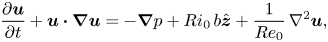 $$\begin{gather} \frac{\partial\boldsymbol{u}}{\partial t}+\boldsymbol{u}\boldsymbol{\cdot}\boldsymbol{\nabla}\boldsymbol{u}={-} \boldsymbol{\nabla} p+Ri_{0}\,b\hat{\boldsymbol{z}}+\frac{1}{Re_{0}}\,\nabla^{2}\boldsymbol{u}, \end{gather}$$
 $$\begin{gather}\frac{\partial b}{\partial t}+\boldsymbol{u}\boldsymbol{\cdot}\boldsymbol{\nabla} b =\frac{1}{Re_{0}\,Pr}\,\nabla^{2}b, \end{gather}$$
 $$\begin{gather}\boldsymbol{\nabla}\boldsymbol{\cdot}\boldsymbol{u}=0, \end{gather}$$
where  $p$ is the pressure, and
  $\hat {\boldsymbol {z}}$ is the vertical unit vector. The equations involve three dimensionless parameters: the initial Reynolds number
  $Re_0=U^{*}_{0}h^{*}/\nu ^{*}$, where
  $\nu ^{*}$ is the kinematic viscosity, the Prandtl number
  $Pr=\nu ^{*}/\kappa ^{*}$, where
  $\kappa ^{*}$ is the diffusivity, and the initial bulk Richardson number
  $Ri_{0}=B^{*}_{0}h^{*}/U^{*2}_{0}$.
In general, we define the gradient Richardson number as
 \begin{equation} Ri_g(z,t)=\frac{\partial \langle b^*\rangle_{xy}/\partial z^*}{(\partial \langle u^*\rangle_{xy}/\partial z^*)^{2}}=Ri_0\,\frac{\partial \langle b\rangle_{xy}/\partial z}{(\partial \langle u\rangle_{xy}/\partial z)^2}=\frac{N^2}{S^2}. \end{equation}
Here, the notation  $\langle \cdot \rangle _{r}$ represents an average over
  $r$, where
  $r$ can encompass any combination of
  $x$,
$x$,  $y$,
$y$,  $z$ and
  $t$. Also,
  $N^2$ is the squared buoyancy frequency, and
  $S$ is the mean shear. The minimum of
  $Ri_g$ with respect to
  $z$ is denoted as
  $Ri_{min}(t)$. In the inviscid limit, a necessary condition for instability is that
  $Ri_{min}$ be less than
  $1/4$ (Howard Reference Howard1961; Miles Reference Miles1961). For the flow described by (2.3), the initial
  $Ri_{min}$ increases from
  $Ri_0/2$ to
  $Ri_0$ when
  $D$ increases from 0 to infinity (figure 2).

Figure 2. The dependence of initial minimum Richardson number  $Ri_{min}$ on
  $D$. Here,
  $Ri_0$ is 0.16.
Boundary conditions are periodic in both horizontal directions, with periodicity intervals  $L_x$ and
  $L_y$. The upper and lower boundaries are free-slip (
 $\partial u/\partial z = \partial v/\partial z = 0$), insulating (
 $\partial b/\partial z = 0$) and impermeable (
 $w=0$).
A small, random velocity perturbation is incorporated into the initial state (2.3). This initial perturbation field is purely stochastic and is applied uniformly to all three velocity components across the computational domain. The maximum amplitude of any single component is limited to 0.05, equivalent to 2.5 % of the velocity change across each shear layer. This magnitude is kept small to ensure that the initial growth phase is consistent with linear perturbation theory. For each value of  $D$, an ensemble of three cases is simulated, each using a distinct seed to generate the random velocities (L22).
2.2. Linear stability analysis
To evaluate the linear instabilities, (2.4)–(2.6) are linearized about the initial base flow (2.3). These equations are then subjected to perturbations induced by small-amplitude, normal mode disturbances proportional to the real part of  $a(z)\exp {(\sigma t+\textrm{i}kx)}$. In this context,
  $a(z)$ denotes the vertically varying, complex amplitude of any perturbation quantity,
  $\sigma$ stands for the complex exponential growth rate, and
  $k$ is the wavenumber in the streamwise direction. The streamwise phase speed is
  $c=\textrm{i}\sigma /k$. The normal mode equations are discretized using a Fourier–Galerkin method, yielding a generalized matrix eigenvalue problem that is solved using standard methods. Details may be found in § 13.3 of Smyth & Carpenter (Reference Smyth and Carpenter2019) or in Lian, Smyth & Liu (Reference Lian, Smyth and Liu2020).
2.3. Direct numerical simulations
Simulations are conducted using DIABLO (Taylor Reference Taylor2008), which utilizes a hybrid implicit–explicit time-stepping scheme with pressure projection. The viscous and diffusive components are addressed implicitly using a second-order Crank–Nicolson method, while other terms are explicitly resolved employing a third-order Runge–Kutta–Wray method. The vertical  $z$ direction dependence is discretized using second-order finite differences, whereas the periodic streamwise and spanwise directions (
 $x, y$) are managed using the Fourier pseudo-spectral method.
To allow subharmonic mode growth, we set the streamwise periodicity interval  $L_x$ to two wavelengths of the fastest-growing KH mode, as determined through linear stability analysis (§ 2.2). For the development of 3-D secondary instabilities, a spanwise periodicity interval of
  $L_y=L_x/4$ is adequate (e.g. Klaassen & Peltier Reference Klaassen and Peltier1985; Mashayek & Peltier Reference Mashayek and Peltier2013). The domain height is
  $L_z=30$ to minimize boundary effects. The computational grid is uniform and isotropic, and resolves
  $\sim$2.5 times the Kolmogorov length scale
  $L_k=(Re^{-3}/\epsilon )^{1/4}$, with
  $\epsilon$ representing a characteristic viscous dissipation rate after turbulence onset (e.g. Smyth & Moum Reference Smyth and Moum2000). Grid sizes are given in table 1.
Table 1. Parameter values for five 3-member direct numerical simulations ensembles. In all cases,  $Re_0=1000$,
  $Pr=1$,
  $Ri_0=0.16$. Data for the case
  $D=\infty$ are sourced from L22 and include only a single, isolated shear layer. The maximum initial random velocity component is 0.05.

Given the sensitivity of turbulent flows to initial conditions, we work with ensemble mean statistics where appropriate. Following L22, we use an ensemble of three cases at each separation distance  $D$. Five values of
  $D$ are considered, for a total of 15 simulations (listed in table 1). We also employ a three-member ensemble of simulations of a single shear layer described in L22 to represent the limiting case
  $D\rightarrow \infty$.
To maintain our primary focus on the influence of the adjacent shear layer, we keep the initial state parameters, specifically the Richardson, Reynolds and Prandtl numbers, fixed. The choice  $Ri_0=0.16$ is large enough for the pairing instability (e.g. Klaassen & Peltier Reference Klaassen and Peltier1989) to be damped by stratification when
  $Ri_{min}=Ri_0$ (i.e. for large
  $D$). In all cases, we set
  $Re_0 = 1000$ and
  $Pr=1$. While smaller than would be typical in nature, these values reflect a necessary compromise dictated by computational resource constraints.
2.4. Diagnostics
The total velocity field can be decomposed into a horizontally averaged component, referred to as the mean flow, and a perturbation
 \begin{equation} \boldsymbol{u}(x,y,z,t)=\bar{U}\,\hat{\boldsymbol{e}}^{(x)}+\boldsymbol{u}'(x,y,z,t), \quad \mathrm{where}\ \bar{U}(z,t)=\left\langle u\right\rangle_{xy}, \end{equation}
with  $\hat {\boldsymbol {e}}^{(x)}$ the unit vector in the streamwise direction. Following Caulfield & Peltier (Reference Caulfield and Peltier2000), the perturbation velocity is further subdivided into two-dimensional (2-D) and 3-D components:
 \begin{equation} \boldsymbol{u}'(x,y,z,t)= \boldsymbol{u}_{2d}+\boldsymbol{u}_{3d}, \end{equation}
where
 \begin{equation} \boldsymbol{u}_{2d}(x,z,t)=\left\langle\boldsymbol{u}\right\rangle_y - \bar{U}\,\hat{\boldsymbol{e}}^{(x)}\quad \mathrm{and}\quad \boldsymbol{u}_{3d}(x,y,z,t)=\boldsymbol{u}-\boldsymbol{u}_{2d}-\bar{U}\,\hat{\boldsymbol{e}}^{(x)}=\boldsymbol{u} - \left\langle\boldsymbol{u}\right\rangle_y. \end{equation}
Similarly, the buoyancy field can be decomposed as
 $$\begin{gather} b(x,y,z,t)=\bar{B}+b'(x,y,z,t), \quad\mathrm{where}\ \bar{B}(z,t)=\langle b\rangle_{xy}, \end{gather}$$
 $$\begin{gather}b_{3d}(x,y,z,t)=b-\langle b\rangle_y. \end{gather}$$
The total kinetic energy can now be partitioned as
 \begin{equation}
\mathscr{K}=\bar{\mathscr{K}}+\mathscr{K}',\quad\mathscr{K}'=\mathscr{K}_{2d}+\mathscr{K}_{3d},
\end{equation}
\begin{equation}
\mathscr{K}=\bar{\mathscr{K}}+\mathscr{K}',\quad\mathscr{K}'=\mathscr{K}_{2d}+\mathscr{K}_{3d},
\end{equation}
where
 \begin{align} \bar{\mathscr{K}}=\tfrac{1}{2}\langle\bar{U}^2\rangle_{z},\quad \mathscr{K}_{2d}=\tfrac{1}{2}\langle u_{2d}^2+v_{2d}^2+w_{2d}^2\rangle_{xz},\quad \mathscr{K}_{3d}=\tfrac{1}{2}\langle u_{3d}^2+v_{3d}^2+w_{3d}^2\rangle_{xyz}. \end{align}
These constituent kinetic energies  $\bar {\mathscr {K}}$,
  $\mathscr {K}'$,
  $\mathscr {K}_{2d}$ and
  $\mathscr {K}_{3d}$ can be identified as the horizontally averaged kinetic energy associated with the mean flow, the turbulent kinetic energy, and the kinetic energy related to 2-D and 3-D motions. We denote the instances in time when
  $\mathscr {K}_{2d}$ and
  $\mathscr {K}_{3d}$ reach their maximum values as
  $t_{2d}$ and
  $t_{3d}$, respectively.
Quantification of irreversible mixing involves decomposing the total potential energy  $\mathscr {P}=-Ri_0\,\langle bz\rangle _{xyz}$ into available and background components,
  $\mathscr {P}=\mathscr {P}_a+\mathscr {P}_b$. The background potential energy
  $\mathscr {P}_b$ is the minimum potential energy achievable by adiabatically rearranging the buoyancy field into a statically stable state
  $b^*$ (Winters et al. Reference Winters, Lombard, Riley and D'Asaro1995; Tseng & Ferziger Reference Tseng and Ferziger2001). After computing the total and background potential energies, the available potential energy is determined from the residual,
  $\mathscr {P}_a=\mathscr {P}-\mathscr {P}_b$. Here,
  $\mathscr {P}_a$ represents the potential energy available for conversion to kinetic energy, arising from lateral variations in buoyancy or statically unstable regions.
The irreversible mixing rate due to fluid motions is defined as
 \begin{equation} \mathscr{M}=\frac{\textrm{d}\mathscr{P}_b}{\textrm{d}t}-\mathscr{D}_p, \end{equation}
where
 \begin{equation} \mathscr{D}_p=\frac{Ri_0\,(b_{top}-b_{bottom})}{Re_0\,Pr\,L_z} \end{equation}
refers to the rate at which the potential energy of a statically stable buoyancy distribution would increase solely due to diffusion of the mean buoyancy profile in the absence of any fluid motion.
There exists a variety of definitions for mixing efficiency in the literature (e.g. Gregg et al. Reference Gregg, D'Asaro, Riley and Kunze2018). Here, we define the instantaneous mixing efficiency as
 \begin{equation} \eta_i = \frac{\mathscr{M}}{\mathscr{M}+\epsilon}, \end{equation}
where  $\epsilon =({2}/{Re})\langle s_{ij}s_{ij}\rangle _{xyz}$ is the total dissipation rate, and
  $s_{ij}=(\partial u_i/\partial x_j+\partial u_j/\partial x_i)/2$ is the strain rate tensor. The mixing efficiency quantifies the fraction of energy directed towards irreversible mixing to the total kinetic energy loss that is irreversibly lost to friction (Peltier & Caulfield Reference Peltier and Caulfield2003). The cumulative mixing efficiency serves as a valuable measure for quantifying the overall efficiency of the entire mixing process, and is defined as
 \begin{equation} \eta_c = \frac{\displaystyle\int\nolimits^{t_f}_{t_i} \mathscr{M} \,\textrm{d}t}{\displaystyle\int\nolimits^{t_f}_{t_i} \mathscr{M} \,\textrm{d}t + \displaystyle\int\nolimits^{t_f}_{t_i} \epsilon \,\textrm{d}t}, \end{equation}
where  $t_i\sim 2$ is the initial time after the model adjustment period, and
  $t_f$ is the final time of the integral at which
  $\mathscr {M}=\mathscr {D}_p$.
An alternative quantifier of mixing that readily shows the spatial structure is the perturbation buoyancy variance dissipation rate, defined as
 \begin{equation} \chi'(x,y,z,t)=\frac{2\,Ri_0}{Re\,Pr}\,|\boldsymbol{\nabla} b'|^2, \end{equation}
where  $b'$ is the buoyancy perturbation, representing the deviation from the horizontal mean buoyancy.
The evolution equation for the kinetic energy of 3-D perturbations can be expressed in the form (Caulfield & Peltier Reference Caulfield and Peltier2000)
 \begin{align} \sigma_{3d}&=\frac{1}{2\mathscr{K}_{3d}}\,\frac{\textrm{d}}{\textrm{d}t}\mathscr{K}_{3d} \end{align}
 \begin{align} &=\mathscr{R}_{3d}+\mathscr{S\!h}_{3d}+\mathscr{A}_{3d}+\mathscr{H}_{3d}+\mathscr{D}_{3d}, \end{align}
where the first two terms represent the 3-D perturbation kinetic energy extraction from the background mean shear and the background 2-D KH billow by means of Reynolds stresses, respectively defined as
 $$\begin{gather} \mathscr{R}_{3d}={-}\frac{1}{2\mathscr{K}_{3d}}\left\langle u_{3d}w_{3d}\,\frac{\partial\bar{U}}{\partial z}\right\rangle_{xyz}, \end{gather}$$
 $$\begin{gather}\mathscr{S\!h}_{3d}={-}\frac{1}{2\mathscr{K}_{3d}}\left\langle u_{3d}w_{3d} \left(\frac{\partial u_{2d}}{\partial z}+\frac{\partial w_{2d}}{\partial x}\right) \right\rangle_{xyz}. \end{gather}$$
The third term represents the stretching deformation of the 3-D motions and is defined as
 \begin{equation} \mathscr{A}_{3d}={-}\frac{1}{2\mathscr{K}_{3d}}\left\langle\frac{1}{2}\left( u_{3d}^2-w_{3d}^2\right) \left(\frac{\partial u_{2d}}{\partial x}-\frac{\partial w_{2d}}{\partial z}\right) \right\rangle_{xyz}. \end{equation}
The final two terms are the buoyancy production term and the negative-definite viscous dissipation term associated with 3-D perturbations, and are defined respectively as
 $$\begin{gather} \mathscr{H}_{3d}=\frac{Ri_0}{2\mathscr{K}_{3d}}\,\langle b_{3d}w_{3d} \rangle_{xyz}, \end{gather}$$
 $$\begin{gather}\mathscr{D}_{3d}={-}\frac{1}{\mathscr{K}_{3d}\,Re}\,\langle s_{ij}s_{ij}\rangle_{xyz}, \end{gather}$$
where  $s_{ij}$ is the strain rate tensor of the 3-D motions. The time at which
  $\sigma _{3d}$ is a maximum is defined as
  $t_{\sigma _{3d}}$. The enstrophy in the three vorticity components is defined as
 \begin{equation} \mathcal{Z}_x=\tfrac{1}{2}(\omega_{x}^2), \quad \mathcal{Z}_y=\tfrac{1}{2}(\omega_{y}^2), \quad \mathcal{Z}_z=\tfrac{1}{2}(\omega_{z}^2), \end{equation}
where
 \begin{equation} \omega_{x}=\frac{\partial w}{\partial y}-\frac{\partial v}{\partial z},\quad \omega_{y}=\frac{\partial u}{\partial z}-\frac{\partial w}{\partial x}\quad \textrm{and}\quad \omega_{z}=\frac{\partial v}{\partial x}-\frac{\partial u}{\partial y}. \end{equation}
3. The primary linear instability
In the extreme cases,  $D=0$ and
  $D\rightarrow \infty$, (2.3) is equivalent to one or two isolated shear layers that produce standard KH instabilities (e.g. Hazel Reference Hazel1972; Smyth & Carpenter Reference Smyth and Carpenter2019) if
  $Ri_0<1/4$. In the previously unexplored cases with finite, non-zero
  $D$, (2.3) represents a superposition of two shear layers whose modes of instability interact in complex ways.
In the case  $D=0$, (2.3) becomes
  $U(z)=B(z)=2\tanh {(z)}$, i.e. the two shear layers sum to make a single stratified shear layer with doubled shear and stratification (dark blue curve in figure 3). The corresponding
  $Ri_{min}$ is
  $Ri_0/2=0.08$. The dominant mode is the stationary KH mode, with a fastest-growing wavenumber 0.44. We term this a stationary mode because there is only a single fastest-growing mode for a given initial state. (This is in contrast to oscillatory instability, discussed below, which is a superposition of two modes with equal growth rates but different phase speeds.) In the reference frame assumed here, the phase speed of the stationary mode is zero, while the two phase speeds of the oscillatory mode are opposites.

Figure 3. Profiles of (a) horizontally averaged velocity and buoyancy, (b) mean velocity and mean buoyancy gradient, and (c) gradient Richardson number. The vertical dashed line in (c) shows  $Ri_0$, and the vertical solid line denotes the stability criterion
  $1/4$.
As  $D$ increases to
  $\tanh ^{-1}\sqrt {1/3}$ (approximately 0.66), the single shear maximum at
  $z=0$ widens (light blue curve in figure 3b). Therefore, the wavenumber of the fastest-growing mode decreases, the growth rate decreases (figure 4, red curve), and
  $Ri_{min}$ increases (figure 3(c), light blue curve). The corresponding mode is a continuation of the stationary mode found at
  $D=0$ as discussed above. It may be thought of as a KH-like instability of the two shear layers in toto, rather than of one or the other layer.

Figure 4. Stability diagram showing the transition from the stationary mode to the oscillatory mode as  $D$ increases, with
  $Re=1000$,
  $Pr=1$,
  $Ri_0=0.16$, and boundaries at
  $z=\pm L_z/2=\pm 15$. Colours and black contours represent the growth rate of the fastest-growing mode on the
  $k\unicode{x2013}D$ plane. The contour interval is 0.02. White contours show the (positive) phase velocity. The horizontal dashed line denotes the critical distance
  $D_c$ (
 $=1.06$). Stars highlight the cases
  $D=0.5$ and
  $D=2$, where the eigenfunctions of the fastest-growing modes are shown in figure 7.
If  $D$ slightly exceeds
  $\tanh ^{-1}\sqrt {1/3}$, then two small shear maxima appear slightly above and below
  $z=0$. These produce two inflectional instabilities having equal (though small) growth rates, and equal but opposite phase velocities. (Only the positive phase velocity is shown in figure 4.) Combined, these modes result in an oscillatory instability. As
  $D$ increases further, the oscillatory and stationary modes coexist (figure 4). The shear maxima become weaker but more distinct (green curve in figure 3b). The growth rate of the oscillatory mode increases, while that of the stationary mode continues to decrease (figure 4). The two modes attain equal growth rates at a critical separation distance
  $D=D_c$, with
  $D_c=1.06$ in the present case,
 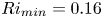 $Ri_{min}=0.16$ (dashed horizontal lines in figures 4 and 5). More generally,
  $D_c$ decreases slightly with increasing
  $Ri_{0}$ (figure 5).

Figure 5. The dependence of critical distance  $D_c$ on
  $Ri_0$. The corresponding
  $D_c$ for
  $Ri_0=0.16$ is
  ${\sim }1.06$, as shown by the red dot.
At higher  $D$ (approximately 1.2 in our case), the stationary mode is stabilized, while the growth rate of the oscillatory mode continues to increase with increasing
  $D$ (figure 4). When
  $D=3$, for example, the two shear maxima are separated by a weakly stratified layer (orange curve in figure 3). The resulting pair of modes have equal growth rates and opposite phase velocities. They combine to form the oscillatory mode. As
  $D\rightarrow \infty$, the upper and lower instabilities that form the oscillatory mode are independent, stationary KH modes with unequal phase speeds.
We next explore the effects of varying  $Ri_0$ (figure 6). When
  $D=0$, the stability boundary for the two superimposed shear layers can be written as
  $Ri_0=2k(1-k)$, neglecting viscosity and assuming an infinite domain (e.g. Smyth & Carpenter Reference Smyth and Carpenter2019). This results in the instability criterion
  $Ri_0<1/2$. Figure 6(a) depicts the growth rate in the
  $k\unicode{x2013}Ri_0$ plane. (Positive values lying outside the theoretical stability boundary are an artefact of the finite vertical domain size; cf. Hazel Reference Hazel1972.) The stationary mode dominates for
  $D=0$ and 0.5 (figures 6a,b). As
  $D$ increases from 0 to 0.5, the unstable modes shift towards lower wavenumbers. When
  $D=1$, the stationary mode is the fastest-growing mode, and its associated fastest-growing wavenumber decreases to less than 0.2 for all
  $Ri_0$ (figure 6c). At higher wavenumbers, the oscillatory mode dominates. With an increase in
  $D$ to 3, the upper and lower shear layers become widely separated, resulting in the disappearance of the stationary mode and the dominance of the oscillatory mode (see figure 6d). The stability boundary under the inviscid limit, depicted as the dashed curve, aligns well with the numerical results. This alignment suggests that, at least within the linear regime, the configuration with
  $D=3$ resembles a pair of isolated shear layers. To summarize, figure 6 shows that the modal structure in the linear regime is remarkably insensitive to the choice of
  $Ri_0$; at each
  $D$, we see only the expected decrease of growth rate with increasing
  $Ri_0$. In what follows, we will focus on the case
  $Ri_0=0.16$.

Figure 6. Stability diagram illustrating the transition from the stationary mode (SM) to the oscillatory mode (OM) as  $D$ increases, with
  $Re=1000$,
  $Pr=1$, and boundaries at
  $z=\pm L_z/2=\pm 15$. Colours and black contours represent the growth rate on the
  $k\unicode{x2013}D$ plane for different values of
  $D$: (a)
  $D=0$, (b)
  $D=0.5$, (c)
  $D=1$, and (d)
  $D=3$. The fastest growth rate at each
  $k, Ri_{0}$ is shown. The contour interval is 0.02. White contours represent the corresponding frequency
  $\sigma _i$. The red curve denotes the fastest-growing mode at each
  $Ri_0$. Dashed curves show the inviscid stability boundary for an infinite domain,
  $Ri_0=2k(1-k)$ when
  $D=0$ in (a), and
  $Ri_0=k(1-k)$ for the single tanh profile considered in (d). The horizontal dashed line and solid line show
  $Ri_0=0.16$ and
  $Ri_0=0.25$, respectively.
We next examine the vertical structures of typical stationary and oscillatory modes. The eigenfunction of the stationary mode at  $D=0.5$ (figure 7a) displays symmetry about
  $z=0$, characteristic of KH instability (e.g. Smyth & Peltier Reference Smyth and Peltier1989). The corresponding phase speed is zero (figure 7a). When
  $D=2$, modes are associated with the upper and lower shear layers. The corresponding eigenfunctions are reflections of each other about
  $z=0$ (figures 7b,c). While upper and lower modes share identical growth rates
  $\sigma _r$, their phase speeds are equal but opposite, so that their sum has an oscillatory, standing-wave-like character.

Figure 7. (a) Magnitudes of the vertical velocity eigenfunction  $\hat {w}$ for the fastest-growing mode when
  $D=0.5$. This mode corresponds to a stationary KH-like instability. (b,c) Magnitudes of the vertical velocity eigenfunction for the upper and lower modes when
  $D=2$. Both of these modes are oscillatory, exhibiting identical growth rates
  $\sigma _r$ and phase speeds
  $c_r$ of equal magnitude but opposite signs.
To close this section, we discuss the mechanisms that cause growth rates to decrease as  $D$ approaches
  $D_c$. As
  $D\rightarrow D_c$ from above, the oscillatory mode is damped. To explain, we invoke the wave resonance mechanism for piecewise linear shear layers (Heifetz et al. Reference Heifetz, Bishop, Hoskins and Methven2004; Carpenter et al. Reference Carpenter, Tedford, Heifetz and Lawrence2013; Heifetz & Guha Reference Heifetz and Guha2019; Smyth & Carpenter Reference Smyth and Carpenter2019). The schematic representation in figure 8(a) shows a piecewise linear velocity profile with four kinks (i.e. vorticity discontinuities). Correspondingly, figure 8(b) depicts the vorticity wave associated with each kink, showing phase-locking between wave 1 and wave 2, as well as between wave 3 and wave 4, each in the phase configuration that is optimal for resonant amplification. This results in the growth of two trains of KH billows, corresponding to the oscillatory instability discussed above. When
  $D$ is finite, an added interaction occurs between wave 2 and wave 3. (Interactions between waves 1 and 3, 2 and 4, and 1 and 4 are present but weaker when
  $D>D_c$.) The phase relationship between these waves now varies in time, owing to their opposing horizontal propagation. Figure 8(b) provides an example. In this particular configuration, waves 2 and 3 force each other in their own directions. The opposite can be true for other phase relationships that occur as the waves pass each other. Regardless of the horizontal propagation, waves 2 and 3 consistently perturb each other's phases, so that they cannot remain phase-locked in the optimal configuration for resonance, and the growth rate is thus reduced. This destructive interference increases as
  $D$ decreases until
  $D=\tanh ^{-1}{\sqrt {1/3}}$, at which point the oscillatory mode vanishes, leaving only the stationary mode.

Figure 8. (a) Piecewise linear background velocity profile. (b) Vorticity wave field diagram. Waves 1 and 2 resonate to create the upper KH-like instability. The phase difference  $0.35{\rm \pi}$ is optimal for growth. The same is true for waves 3 and 4, which create the lower KH-like instability. The main interaction between these two instabilities involves waves 2 and 3. Counter-rotating vorticity perturbation causes alternately upward and downward motion (black solid arrows). These motions induce vertical motions to the nearby waves (black dashed arrows). Therefore, the interaction accelerates the upper wave to the left (blue arrows) and the lower wave to the right (red arrows).
The damping that we find as  $D\rightarrow D_c$ from below (figure 4) is unsurprising because the shear maximum at
  $z=0$ weakens (figure 3(b), compare dark blue and light blue curves), but it can also be understood in terms of wave resonance. The resonance between wave 1 and wave 2, as well as between wave 3 and wave 4, diminishes due to the disturbances between waves 2 and 3 described above. However, resonance between wave 1 and wave 4 remains strong, leading to the development of a KH-like instability. As
  $D\rightarrow D_c^-$, the separation between wave 1 and wave 4 increases, rendering resonance less effective.
4. The route to turbulence
4.1. Overview of the nonlinear development
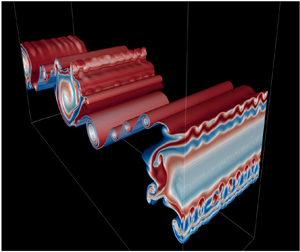
In this subsection, we look beyond the linear regime to examine the various secondary instabilities that emerge at different separation distances  $D$ and trigger the transition to turbulence (see examples in figure 9). In all cases, the initial condition consists of an unstable parallel shear flow whose primary instability grows to form 2-D periodic laminar vortices. These vortices attain maximum kinetic energy at
  $t=t_{2d}$ (figures 9a,e,i). As expected, the wavelength is largest (among these three examples) for
  $D=1$, and smallest for
  $D=2$, where two trains of billows combine to form the oscillatory instability (figure 9i). In the oscillatory case,
  $D=2$, the growth rate and the time of turbulence onset are sensitive to the details of the initial perturbations, as is evident in the contrast between the upper and lower billow trains (figures 9i,j). The evolution progresses at a comparatively slower rate for
  $D=1$, consistent with its relatively small linear growth rate, while growth is faster for
  $D=0.5$ (compare the values of
  $t_{2d}$ between cases). During this progression, various secondary instabilities emerge, facilitating the breakdown of the primary KH billows (e.g. figures 9b,f,j). This breakdown leads to the generation of turbulence (e.g. at
  $t=t_{3d}$, figures 9c,g,k). Following the turbulent mixing phase, the flow relaminarizes (figures 9d,h,l).

Figure 9. Cross-sections through the 3-D buoyancy field for example cases with (a–d)  $D=0.5$, (e–h)
  $D=1$, and (i–l)
  $D=2$, at successive times as indicated. The buoyancy values plotted range from
  $-1.5$ (blue) to 1.5 (red). Snapshots in (a,e,i) correspond to
  $t=t_{2d}$, in (c,g,k) to
  $t=t_{3d}$, and in (d,h,l) to
  $t=t_f$, the time when
  $\mathscr {M}=\mathscr {D}_p$.
Secondary instabilities that govern the evolution of isolated KH billows at different values of  $Ri_{min}$ have been explored in previous research (e.g. Davis & Peltier Reference Davis and Peltier1979; Klaassen & Peltier Reference Klaassen and Peltier1985, Reference Klaassen and Peltier1991; Mashayek & Peltier Reference Mashayek and Peltier2012a,Reference Mashayek and Peltierb, Reference Mashayek and Peltier2013, L22). In §§ 4.2 and 4.3, we focus on secondary instabilities that contribute to 3-D perturbation kinetic energy in the regimes
  $D>D_c$ and
  $D< D_c$, wherein the linear development is dominated by the oscillatory and stationary modes, respectively. Pertinent examples include the central core instability (CCI, e.g. Klaassen & Peltier Reference Klaassen and Peltier1991, L23), which is catalysed by the initial growth of the KH instability, and the shear-aligned convective instability (SCI, e.g. Davis & Peltier Reference Davis and Peltier1979; Klaassen & Peltier Reference Klaassen and Peltier1985), which manifests when KH billows reach a sufficient size to overturn the buoyancy structure. In § 4.4, we discuss 2-D secondary instabilities: the secondary shear instability (SSI) of the braids and pairing of adjacent billows (visible in figures 9(f) and 9(b), respectively).
4.2. Regime  $D>D_c$

We examine the regime  $D>D_c$, using ensembles of simulations with
  $D\rightarrow \infty$,
  $D=3$ and
  $D=2$ as examples. When the shear layers are infinitely separated (
 $D\rightarrow \infty$), they are independent of each other, and each exhibits the standard KH instability (e.g. L22). The 3-D perturbation kinetic energy
  $\mathscr {K}_{3d}$ (figure 10a) is created mostly by shear production
  $\mathscr {R}_{3d}$, which draws energy from the mean flow (blue curve). The growth of
  $\mathscr {R}_{3d}$ can be attributed to the sinusoidal distortion of the spanwise vortex tube at the core of each nascent KH billow, which redirects spanwise (
 $\kern0.7pt y$) vorticity towards the
  $x\unicode{x2013}z$ plane. The tilt of the sinusoidal distortion is such that the Reynolds stress
  $\langle u_{3d}w_{3d}\rangle _{xyz}$ becomes negative (see figure 14 of Lasheras & Choi (Reference Lasheras and Choi1988), figure 9 of Smyth & Winters (Reference Smyth and Winters2003), or figure 8 of Smyth Reference Smyth2006). This negative 3-D stress field works with the positive mean shear
  $\textrm{d}\bar {U}/\textrm{d}z$ to generate 3-D kinetic energy. By
  $t=t_{\sigma _{3d}}$ (the time of maximum 3-D growth),
  $\textrm{d}\bar {U}/\textrm{d}z$ is no longer a maximum in the billow core, but the Reynolds stress is. Therefore, the dominant contributor to energy growth, quantified by
  $\mathscr {R}_{3d}$, arises in this region. We identify this mode as the CCI.

Figure 10. Time variation of terms of the  $\sigma _{3d}$ equation (2.21) when (a)
  $D=\infty$, (b)
  $D=3$, and (c)
  $D=2$. All curves are ensemble averaged. Vertical dashed lines show the time at which the growth
  $\sigma _{3d}$ is a maximum. Note that the time for each ensemble case is shifted, such that the 3-D growth rate
  $\sigma _{3d}$ is a maximum at
  $t-t_{\sigma _{3d}}=0$. Terms except for
  $\sigma _{3d}$ are obtained from cubic spline fits.
The buoyancy production  $\mathscr {H}_{3d}$ (red curve) is positive but much smaller than
  $\mathscr {R}_{3d}$. In the current case with
  $Ri_0=0.16$, previous work suggests that the SCI (signalled by positive
  $\mathscr {H}_{3d}$) should be suppressed. Based on secondary stability analysis, the SCI grows only when
  $0.065< Ri_0<0.13$ (Klaassen & Peltier Reference Klaassen and Peltier1991). The dominance of shear production
  $\mathscr {R}_{3d}$ and suppression of buoyancy production
  $\mathscr {H}_{3d}$ when
  $D\rightarrow \infty$ are also consistent with the findings of Mashayek, Caulfield & Peltier (Reference Mashayek, Caulfield and Peltier2013), particularly in their case
  $Ri_0=0.16$,
  $Re=6000$.
As the separation distance between two shear layers is decreased from infinity to values approaching  $D_c$ (e.g. our examples
  $D=3$ and 2), interactions become evident. When
  $D=3$, the evolution of each perturbation energy term resembles the infinite separation case (compare figures 10a,b), suggesting only a weak interaction between the upper and lower instabilities. When
  $D=2$,
  $\mathscr {R}_{3d}$ remains the dominant term (i.e. the principal secondary instability is still the CCI); however, a reduction in
  $\mathscr {H}_{3d}$ (figure 10c) is observed. At
  $t=t_{\sigma _{3d}}$, for example, the reduction is
  ${\sim }40\,\%$ compared to case
  $D\rightarrow \infty$. This reduction can be attributed to the close proximity of the shear layers, which results in additional suppression of SCI beyond the inherent effects of high
  $Ri_{min}$. Because the upper and lower billows co-rotate, roll-up is suppressed, reducing overturning. This is reminiscent of the effect of a nearby boundary on the SCI (L23).
4.3. Regime $D< D_c$

We now examine distinctions that arise when  $D< D_c$, using examples
  $D=0$,
  $0.5$ and 1. When
  $D=0$, the two shear layers add to form a single shear layer with
 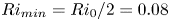 $Ri_{min}=Ri_0/2=0.08$. Thus the instability behaves similarly to a weakly stratified shear instability, and we expect to encounter the SCI. During the earliest stage of 3-D growth (
 $t-t_{\sigma _{3d}}\sim -18$ to
  $-6$), the
  $\mathscr {K}_{3d}$ budget is dominated by the shear production term
  $\mathscr {R}_{3d}$ due to the CCI. By
  $t \sim t_{\sigma _{3d}}$, the billow has rolled up enough to form convectively unstable layers. Consistent with the low initial
  $Ri_{min}$, the SCI is now the principal secondary instability that breaks down the KH billow structure. This is indicated in the
  $\mathscr {K}_{3d}$ budget (figure 11) by increased values of
  $\mathscr {H}_{3d}$ as well as
  $\mathscr {S\!h}_{3d}$ and
  $\mathscr {A}_{3d}$. One would expect the buoyancy production term
  $\mathscr {H}_{3d}$ to be substantial due to the prevailing influence of the SCI (Caulfield & Peltier Reference Caulfield and Peltier2000, L23). Surprisingly, both
  $\mathscr {S\!h}_{3d}$ and
  $\mathscr {A}_{3d}$ exhibit larger magnitudes than
  $\mathscr {H}_{3d}$ (figure 11a). This finding is distinguished from previous studies (Mashayek & Peltier Reference Mashayek and Peltier2013, L23), where buoyancy production dominated in the presence of the SCI. This may reflect a difference in the initial perturbations; the buoyancy field was perturbed in the previous studies but not in the present work.

Figure 11. As in figure 10, but with  $D=0$.
When  $D$ is slightly above 0 (typified here by
  $D=0.5$),
  $Ri_{min}$ is small enough that the KH billow is again susceptible to SCI (Klaassen & Peltier Reference Klaassen and Peltier1991). During the initial growth phase (dot-dashed line in figure 12a), large positive values of
  $\mathscr {R}_{3d}$ concentrate in the billow core, indicating the CCI. This mechanism can be discerned qualitatively in the spanwise-averaged
  $x\unicode{x2013}z$ representation of
  $\mathscr {R}_{3d}$ (figure 12(b), region 1). Simultaneously, small areas of positive
  $\mathscr {S\!h}_{3d}$ manifest at the upper and lower extents of the billows (figure 12(c), region 2). Moreover, positive
  $\mathscr {A}_{3d}$ emerges along the braids (figure 12(d), region 3). These results are associated with the mechanism illustrated in figure 12 of Lasheras & Choi (Reference Lasheras and Choi1988), which shows that vortex filaments present in the braids undergo amplification through stretching along the principal plane of positive strain. These vortex filaments eventually envelop the spanwise vortex tubes of the central core, resulting in positive
  $\mathscr {S\!h}_{3d}$ in the upper and lower regions of each billow, and positive
  $\mathscr {A}_{3d}$ at the braids. Owing to the wrapping of these vortex filaments, the spanwise vortex tubes undulate (figure 14 in Lasheras & Choi Reference Lasheras and Choi1988), creating positive
  $\mathscr {R}_{3d}$ in the core. Nonetheless,
  $\mathscr {S\!h}_{3d}$ is mostly negative in the braids and in the billow cores, leading to an overall negative volume average (dashed line in figure 12a). Positive
  $\mathscr {H}_{3d}$ in the eyelids (region 4 of figure 12e) indicates the SCI.

Figure 12. Dominant stationary mode when  $D=0.5$. (a) As in figure 10. Vertical dot-dashed line and dashed line show the times at
  $t-t_{\sigma _{3d}}=-11$ and 0, respectively. (b–e) Spatial distribution of each energy term:
  $\mathscr {R}_{3d}$,
  $\mathscr {S\!h}_{3d}$,
  $\mathscr {A}_{3d}$ and
  $\mathscr {H}_{3d}$, respectively, at
  $t_{\sigma _{3d}}=-11$ (dot-dashed line in a). (f–i) Same at
  $t-t_{\sigma _{3d}}=0$ (dashed line in a).
At  $t=t_{\sigma _{3d}}$, similar to
  $D=0$,
  $\mathscr {H}_{3d}$ is smaller than both
  $\mathscr {S\!h}_{3d}$ and
  $\mathscr {A}_{3d}$ (figure 12a). The SCI induces the formation of shear-aligned convective rolls, consistent with increased buoyancy production
  $\mathscr {H}_{3d}$ (figure 12(i), region 7). Positive
  $\mathscr {S\!h}_{3d}$ coincides with these convective rolls (region 5), suggesting that the SCI could be responsible for its generation. During the early growth phase,
  $\mathscr {H}_{3d}$ (region 4) begins to increase on the eyelids of each billow, whereas
  $\mathscr {S\!h}_{3d}$ remains small or negative in that area (figure 12c). This implies that as time progresses, the increase in positive
  $\mathscr {S\!h}_{3d}$ on the eyelids results from the formation of shear-aligned convective rolls with circulations tilted against the 2-D shear (figure 13). Vortex tubes at the periphery of the billows also undergo stretching, as quantified by
  $\mathscr {A}_{3d}$. Stretching occurs when denser fluid descends on the upper right portion of the billow under the action of gravity, while lighter fluid ascends on the lower left (figure 12(h), region 6).

Figure 13. Schematic showing shear-aligned convective rolls tilting and stretching to form positive  $\mathscr {S\!h}_{3d}$ and
  $\mathscr {A}_{3d}$, respectively.
During this phase of maximum growth, negative  $\mathscr {R}_{3d}$ emerges at the margins of the billows (figure 12f). Consequently, the volume-averaged value is negative (figure 12(a), indicated by the blue curve at
  $t=t_{\sigma _{3d}}$). This suggests that the background mean flow contributes little to the 3-D perturbation kinetic energy in this instance. Instead, the perturbation energy is partially created by buoyancy production, but is predominantly due to shear production and the stretching of vortex tubes as discussed above.
In the case  $D=1$, although the oscillatory mode is unstable, the dynamics is governed primarily by the stationary mode. The perturbation energy terms evolve similarly to the case
  $D=0.5$ (compare figures 12(a) and 14). This is interesting because
  $Ri_{min}=0.15$, which is outside the range 0.065–0.13 where the SCI is expected based on secondary stability analysis of an isolated shear layer (Klaassen & Peltier Reference Klaassen and Peltier1991), yet the roll motions are visible, for example, on the right-hand face of figure 9(f). We conclude that as in the case
  $D=0.5$, the SCI gives rise to shear-aligned convection rolls, consistent with positive values of
  $\mathscr {H}_{3d}$. The dominant source terms are again
  $\mathscr {S\!h}_{3d}$ and
  $\mathscr {A}_{3d}$ (figure 14).

Figure 14. Dominant stationary mode when  $D=1$. As in figure 10.
4.4. The SSI and pairing
We discuss the SSI and pairing separately as they affect  $\mathscr {K}_{3d}$ negligibly. The SSI grows on the braids of the primary billows where the flow is nearly parallel and the shear is intensified by the strain of the large billows (Corcos & Sherman Reference Corcos and Sherman1976; Staquet Reference Staquet1995; Smyth Reference Smyth2003; Mashayek & Peltier Reference Mashayek and Peltier2012a). Staquet (Reference Staquet1995) and Smyth (Reference Smyth2003) find that the SSI tends to occur at higher
  $Re_0$. When
  $D< D_c$, the initial mean flow resembles a single shear layer with increased thickness and velocity change, i.e. with a larger Reynolds number. Therefore, the SSI may occur, depending on the initial noise field. An example is seen in figure 9(f). This secondary instability plays a notable role in generating turbulent mixing (to be discussed in § 5). At
  $t=t_{\sigma _{3d}}$, when
  $\sigma _{3d}$ is a maximum, the enstrophy of the spanwise component
  $\mathcal {Z}_y$ (figure 15b) is significantly stronger than that of the other two components combined,
  $\mathcal {Z}_x+\mathcal {Z}_z$ (figure 15a). The same is true for later times (figures 15(c,d) in the SSI-affected region), further confirming the 2-D nature of the SSI.

Figure 15. Spatial distribution of enstrophy during and after maximum secondary instability growth. Data are from a sample simulation in the  $D=1$ ensemble: (a,c)
  $x$ and
  $z$ components combined; (b,d)
  $y$ component. (a,b) are both at
  $t-t_{\sigma _{3d}}=0$, and (c,d) are at
  $t-t_{\sigma _{3d}}=7$. Horizontal streaks are artefacts of limited spatial resolution.
Secondary billows can be created either in pairs straddling the braid stagnation point or individually (Smyth Reference Smyth2003), as seen at  $t-t_{\sigma _{3d}}=7$ in figure 15(d). Between the large billow cores, a pair of smaller billows emerges at the stagnation point. The pair eventually merges and becomes a larger single vortex, which then creates its own tertiary shear instability in its surroundings, a vivid illustration of a self-similar downscale energy cascade. Other secondary billows developed away from the stagnation point are advected outwards by the extensional strain.
Vortex pairing is also affected by a nearby shear layer. Pairing is more likely to occur when  $D$ is small (e.g.
  $D=0$ and 0.5), due to small
  $Ri_{min}$ (figure 9b). L22 found that pairing is laminar (i.e. it occurs prior to the onset of turbulence) in cases with
  $Ri_{min}$ less than 0.14, and we expected this to remain true in the present cases where
  $Ri_{min}$ is considerably smaller. However, figure 9(c) indicates turbulent pairing. This is likely due to the difference in shape between the present shear layer and the single hyperbolic tangent profile assumed in L22. When
  $D\sim 0$, pairing precedes the onset of the SSI, leading to the disappearance of alternate braids. Subsequently, if the braids are not yet turbulent, then the SSI is likely to appear. The timing of turbulence onset, which itself depends on the choice of initial perturbation (L22), partly determines the occurrence of pairing and the SSI.
5. Turbulent mixing
A neighbouring unstable shear layer could influence turbulent mixing through its impact on the route to turbulence. We test this possibility by investigating three mixing properties: the mixing rate  $\mathscr {M}$, the dissipation rate
  $\epsilon$, and the mixing efficiency
  $\eta$, in both instantaneous (figure 16) and cumulative (figure 18) forms.

Figure 16. Time variation of the instantaneous (a) mixing rate, (b) total dissipation of the kinetic energy, and (c) mixing efficiency, with varying  $D$. For clarity, only one ensemble member is included for each case of different
  $D$. Note that the magnitude and timing of the peak can be slightly different, but the overall trend is similar between the ensemble cases. The solid and dashed black curves are the case with the isolated shear layer. A running mean is carried out for all curves. Diamonds correspond to the snapshots in figure 17.

Figure 17. An  $x\unicode{x2013}z$ slice of the buoyancy variance dissipation rate
  $\log \chi '$ when the instantaneous mixing efficiency
  $\eta _i$ is a maximum for (a)
  $D=0.5$, (b)
  $D=1$, (c)
  $D=2$, and (d)
  $D=3$. The snapshots for different
  $D$ cases correspond to the diamond symbols in figure 16. In (b), horizontal streaks are artefacts of limited spatial resolution.
5.1. Instantaneous mixing properties
We first examine cases with an isolated shear layer, namely,  $D=0$ and
  $D\rightarrow \infty$, to set the stage for cases with
  $D\sim O(1)$. When
  $D=0$, mixing efficiency peaks as the billows roll up (
 $t\sim 60$, black curve in figure 16c). At this pre-turbulent stage, the mixing rate is large (figure 16a) due to sharp scalar gradients, while the dissipation rate (figure 16b) remains small, and mixing efficiency is therefore large (Winters et al. Reference Winters, Lombard, Riley and D'Asaro1995; Caulfield & Peltier Reference Caulfield and Peltier2000; Smyth & Moum Reference Smyth and Moum2001; Smyth Reference Smyth2020). Subsequently, the billow structure collapses due to the SCI (§ 4), leading to an increase in both mixing and dissipation rates. Thus mixing efficiency is reduced at
  $t\sim 70$ as the flow becomes turbulent. As the billows pair and merge into a single large vortex (
 $t\sim 110$), the mixing and dissipation rates begin to rise.
In the case  $D\rightarrow \infty$,
  $Ri_{min}$ doubles to 0.16. Therefore, mixing is visibly weaker than at
  $D=0$ (compare black solid and dashed curves in figure 16a). However, since the dissipation rate is also smaller, the peak mixing efficiency at
  $t\sim 208$ (
 $\eta _i=0.63$) for
  $D\rightarrow \infty$ is not very different from the peak value for
  $D=0$ at
  $t\sim 62$ (
 $\eta _i=0.78$). The two peaks of
  $\mathscr {M}$ are associated respectively with the breakdown of the billow and with mixing due to fully developed turbulence (cf. Kaminski & Smyth Reference Kaminski and Smyth2019, L23).
When  $D=0.5$, the mixing characteristics resemble those at
  $D=0$. Mixing efficiency exhibits a peak during roll-up (as
  $t=76$, marked by the blue diamond in figure 16c). Strong mixing, quantified by the buoyancy variance dissipation rate
  $\chi '$ (2.19), begins along the braids and extends inwards through overturned layers surrounding the core (figure 17a).
When  $D=1$, the time at which the billows roll up is the latest compared with other cases of
  $D$, consistent with its smallest growth rate (figure 4). The increase of mixing efficiency begins at
  $t\sim 180$ (red curve in figure 16c). Subsequently, the mixing rate increases rapidly due to the amplifying KH billow. At
  $t=217$, the 2-D kinetic energy reaches its maximum, while dissipation remains relatively weak, accounting for the highly efficient mixing. Before the SCI collapses the KH billow structure, the SSI emerges along the braids. The emergence of the SSI leads to a surge of highly efficient mixing (
 $t=215\unicode{x2013}235$ in figure 16a). Mixing is most intense in the braids, where it coincides with the secondary KH billows (figure 17b), and is most efficient at
  $t=235$ (red diamond) because the secondary billows have not yet become turbulent, with
  $\eta _i\sim 0.8$ (figure 16c).
The SSI billows travel along the braids towards the primary KH billow, and then intermingle with the shear-aligned convective rolls at the eyelids (at  $x=40$, figure 17b). The primary KH billow then collapses, and the flow becomes more turbulent (
 $t\sim 250$). At this time, the mixing and dissipation rates approach their peak values, coinciding with a precipitous drop in the mixing efficiency (figure 16c).
The regime  $D>D_c$, in which the oscillatory instability dominates (§ 3), is typified here by the cases
  $D=2$ and
  $D=3$. Both the mixing rate and dissipation rate are weak compared to cases where stationary mode dominates, e.g.
  $D=0$,
  $0.5$ and 1 (figures 16a,b). This weakening is due to the stronger stratification, which tends to damp both the SCI and pairing. In addition, the mutual interference of neighbouring billows suppresses the growth of the primary KH instability, leading to reduced overturning and 3-D convection, hence smaller
  $\mathscr {M}$ (compare
  $D=2$ and
  $D=\infty$ in figure 18a).

Figure 18. Dependence of (a) cumulative mixing, (b) cumulative dissipation, and (c) cumulative mixing efficiency on  $D$. All ensemble cases are plotted. Red curves are the ensemble mean. The end time for the time integral is when
  $\mathscr {M}=\mathscr {D}_p$. The vertical dashed lines denote the critical separation distance
  $D_c$. The horizontal line denotes the canonical
  $\eta _c=1/6$ suggested by Osborn (Reference Osborn1980).
While the general pattern of mixing, dissipation, and mixing efficiency remains largely consistent across all cases when  $D>D_c$, there is a reduction in mixing efficiency as
  $D\rightarrow D_c^+$ (compare peak values for
  $D=\infty$,
  $D=3$ and
  $D=2$ in figure 16c). This reduction mainly reflects the diminished mixing rate
  $\mathscr {M}$ observed at smaller values of
  $D$. As shown in figures 17(c) and 17(d),
  $\chi '$ is less pronounced in case
  $D=2$ compared to case
  $D=3$. This suggests that as the nonlinear interaction between the upper and lower shear layers intensifies, mixing is suppressed.
5.2. Cumulative mixing properties
We next investigate the dependence of the cumulative mixing ( $\mathscr {M}_c$), dissipation (
 $\epsilon _c$) and mixing efficiency (
 $\eta _c$) on the separation distance
  $D$. When
  $D< D_c$, the net mixing and dissipation are
  $\sim$1 order of magnitude larger than when
  $D>D_c$ (figures 18a,b). There is less disparity in
  $\eta _c$, indicating an approximate balance between mixing and dissipation that tends to preserve mixing efficiency. Even so, mixing is typically more efficient by a factor
  $\sim$2 when
  $D< D_c$ compared to when
  $D>D_c$. At the extremes
  $D=0$ and
  $D\rightarrow \infty$,
  $\eta _c$ takes the high values (0.3–0.4) expected for an isolated shear layer (Winters et al. Reference Winters, Lombard, Riley and D'Asaro1995; Caulfield & Peltier Reference Caulfield and Peltier2000; Smyth, Moum & Caldwell Reference Smyth, Moum and Caldwell2001).
In the oscillatory regime, the overall reduction in total amount of mixing as  $D$ approaches
  $D_c$ from above may be attributed to the suppression of both the primary KH instability (due to interference between neighbouring billows impeding the phase-locking of resonant waves, as discussed in § 3) and secondary instabilities. The SCI, which plays a major role in driving mixing, can be impacted by both the reduced overturning in the suppressed primary KH instability and the neighbouring effect (§ 4.2). This suppression of the SCI becomes more pronounced as
  $D\rightarrow D_c^+$, potentially leading to a complete prevention of mixing – auxiliary simulations with
  $D=1.5$, not shown here, failed to generated detectable instability or mixing. While
  $\mathscr {M}_c$ decreases as
  $D\rightarrow D_c^+$, there is little corresponding change in total dissipation (figure 18b), leading to an overall decrease in mixing efficiency.
In the stationary regime  $D< D_c$, there is a slight tendency towards stronger mixing and dissipation (figures 18a,b) with decreasing
  $D$. This is likely associated with the slight reduction of
  $Ri_{min}$.
5.3. Emergence of marginal instability
Geophysical stratified shear flows are often in a state of marginal instability (MI), wherein the mean flow fluctuates around a stability boundary approximated by  $Ri_g=1/4$ (see Smyth (Reference Smyth2020), for a recent review). In the present simulations, we find MI-like behaviour when
  $D=2$ (figures 19b,e,h). As turbulence decays (
 $t\sim 250$), a layer of near-critical
  $Ri_g$ (i.e. clustered around a value near
  $1/4$) emerges around
  $z=0$ (figure 19(b), symbol
  ${\textsf{x}}$). This near-critical
  $Ri_g$ corresponds to a new stratified shear layer that forms between the two original layers (figures 19e,h) as mixing brings fluid from the upper and lower turbulent layers into close contact in the middle region, leading to local amplification of the mean buoyancy and velocity gradients.

Figure 19. Horizontally averaged time series of (a–c)  $Ri_g$, (d–f)
  $N^2$, and (g–i)
  $S^2$. The symbol
  $\textsf{x}$ indicates the potential location for MI to occur.
The MI appears only in a restricted range of  $D$, namely when the instability is in the oscillatory regime (
 $D>D_c$) but
  $D$ is not much greater than
  $D_c$. Conversely, for
  $D< D_c$, the mixing characteristics resemble those of a typical KH instability, where both stratification and shear are smoothed due to strong overturning (figures 19d,g). This leads to an increase of
  $Ri_g$ towards a stable state (figure 19a). When
  $D$ is much greater than
  $D_c$, e.g.
  $D=3$, the upper and lower shear layers remain too distant to overlap despite their expansion. Consequently, the weakly stratified and weakly sheared middle layer (at
  $z=0$) persists (figures 19f,i) such that
  $Ri_g$ is much greater than
  $1/4$ (figure 19c).
6. Summary
We have investigated the instabilities of a pair of shear layers. When the layers are either unseparated or separate to an infinite extent, flow evolution is driven by the classical KH instability. Our primary focus, however, is cases characterized by a finite, non-zero separation distance  $D$.
$D$.
In the small-amplitude limit, we find two distinct regimes: (1) a stationary mode, defined by a unique maximum growth rate, dominates when  $D< D_c$ (where
  $D_c\approx 1$ is the critical separation distance); and (2) an oscillatory mode, consisting of two modes with equal growth rates and different phase speeds, becomes unstable when
  $D > \tanh ^{-1}{\sqrt {1/3}}$, and dominates when
  $D>D_c$. As
  $D\rightarrow D_c$ from below, the stationary mode is damped because the shear maximum weakens. As
  $D\rightarrow D_c$ from above, damping of the oscillatory mode can be understood in terms of the resonant interaction of vorticity waves.
The presence of a neighbouring shear layer alters mixing and its efficiency by introducing an alternative route to turbulence. We have extended our analysis beyond the linear regime by conducting an ensemble of three direct numerical simulations, with different initial perturbations, for each of five values of the separation distance  $D$. The presence of a neighbouring shear layer exerts a profound influence on the evolution and wavelength of the primary instability as well as the amplitude of the resulting KH billows. The KH instability evolves most rapidly when
  $D$ is close to 0, consistent with its largest growth rate. As
  $D$ increases from 0 to
  $D_c$, the evolution of the instability is prolonged (consistent with its decreasing growth rate), and the wavelength and amplitude of the KH billows increase. As
  $D$ increases further from
  $D_c$ to infinity, the evolution time and wavelength of the instability converge to values characteristic of an isolated shear layer.
The value of  $Ri_{min}$ is higher in the oscillatory regime (
 $D>D_c$) and lower in the stationary regime (
 $D< D_c$). Important differences in both the route to turbulence and the resulting mixing can be traced back to this distinction. In the oscillatory regime,
  $Ri_{min}\approx Ri_0$, the SCI is suppressed due to both the influence of stratification (Klaassen & Peltier Reference Klaassen and Peltier1991) and interference from the adjacent shear layer. The CCI is now dominant. Mixing is relatively weak and inefficient. When the separation between the upper and lower shear layers is sufficiently small, a new shear layer, exhibiting MI, forms between them.
In the stationary regime ( $D< D_c$),
  $Ri_{min}$ is lower and the instability resembles a weakly stratified KH instability with large amplitude. The SCI creates shear-aligned convective rolls, leading to an increase in buoyancy production (similar to previous studies, e.g. Caulfield & Peltier Reference Caulfield and Peltier2000, L23). Additionally, owing to weak stratification, billows are likely to pair. As
  $D$ approaches
  $D_c$ from below, buoyancy production becomes less important while shear production and gravitational stretching take over as the primary mechanisms of 3-D growth. The SSI, while not contributing directly to 3-D perturbation kinetic energy, plays a significant role in generating turbulence.
The stationary mode leads to strong and efficient mixing. At the transition to the oscillatory regime, the cumulative mixing rate, dissipation rate and mixing efficiency all decrease abruptly (figure 18c), showing that mixing properties can be sensitive to small changes in the initial mean flow.
7. Future directions
In this study, the initial parameters  $Ri_0$,
  $Re_0$ and
  $Pr$ remain constant, with our primary focus on the impact of separation distances. Changing these parameters will alter the transition process in various ways. For example, a different
  $Ri_0$ may alter the growth of KH instability, subharmonic instability and 3-D secondary instabilities. Turbulent mixing and the potential for marginal instability would consequently be affected in ways that are difficult to anticipate. Moreover, varying
  $Ri_0$ while fixing
  $Ri_{min}$ could isolate the effect of the separation distance
  $D$.
$D$.
Increasing  $Re_0$ is essential for simulating geophysical flows. This increase introduces a variety of secondary instabilities, which could be affected by the presence of a neighbouring shear instability. The increase of
  $Re_0$ facilitates exploration of approaching the critical separation distance (
 $D\sim D_c$), as the KH instability may transition to turbulence even when heavily damped by a neighbouring instability.
While  $Pr=1$ is applicable to air, higher values are more realistic for water. A higher
  $Pr$ opens the possibility of a Holmboe-like instability when the mean buoyancy changes more abruptly with height than does velocity. Future studies will explore interactions of nearby Holmboe instability. This may give rise not only to KH-like instability (involving vorticity wave interaction) and Holmboe-like instability (involving vorticity and gravity wave interaction) but also to Taylor–Caulfield instability (interaction between two gravity waves; see Lee & Caulfield Reference Lee and Caulfield2001; Smyth & Carpenter Reference Smyth and Carpenter2019), depending on the separation distance. Moreover, the scouring motion induced by Holmboe waves could be affected by the adjacent shear instability.
The variability in mixing parameters at varying separation distances has significant implications for the estimation of mixing in geophysical flows, particularly those characterized by the presence of neighbouring shear instabilities (e.g. Desaubies & Smith Reference Desaubies and Smith1982; Moum et al. Reference Moum, Nash and Smyth2011). For the parameter values used here, the mixing efficiency ranges from  ${\sim }0.14$ to
  ${\sim }0.37$, depending on the separation distance (figure 18c). Under different initial parameters or varied profile structures, such as asymmetrical velocity and buoyancy profiles (e.g. Olsthoorn, Kaminski & Robb Reference Olsthoorn, Kaminski and Robb2023), the resulting mixing could also be substantially affected by a neighbouring instability.
The exploration of the parameter space will ultimately support a comprehensive parametrization framework for capturing the influence of neighbouring shear layers in a larger-scale model. A future goal is to explore these effects in a multi-layer context, such as the interaction of breaking internal waves at ocean ridges and seamounts.
Pre-existing turbulence exerts a substantial influence on KH instabilities (Brucker & Sarkar Reference Brucker and Sarkar2007; Kaminski & Smyth Reference Kaminski and Smyth2019). Furthermore, the onset timing of shear-driven turbulence is inherently arbitrary, making the simultaneous instability of two adjacent shear layers an atypical scenario. This highlights the potential impact of a near-field turbulent event on pre-turbulent shear instabilities. Such events may alter the development of turbulence in an adjacent shear layer.
Forced stratified flows may organize into layers consisting of neighbouring strongly stratified interfaces separated by regions of weak stratification, and a significant effort has been made to understand the circumstances under which these layers form and survive (Caulfield Reference Caulfield2021; Petropoulos, Mashayek & Caulfield Reference Petropoulos, Mashayek and Caulfield2023). While layered structures may be robust in certain scenarios, particularly in high- $Pr$ and double-diffusive flows (Timmermans et al. Reference Timmermans, Toole, Krishfield and Winsor2008; Taylor & Zhou Reference Taylor and Zhou2017), in other scenarios they are prone to destruction by shear. Recent efforts have described, for example, the interaction between double-diffusive staircase structures and shear-driven turbulence (e.g. Bebieva & Speer Reference Bebieva and Speer2019; Brown & Radko Reference Brown and Radko2022). In the present problem, increasing the number of layers could provide insight into the development of turbulence in these multilayered flows.
Supplementary movies
Supplementary movies are available at https://doi.org/10.1017/jfm.2024.387.
Acknowledgements
This paper is part of the first author's PhD thesis at Oregon State University. We appreciate useful input from advisory committee members J. Moum, J. Liburdy, J. Nash and B. Pearson. We appreciate J. Carpenter's advice on the damping of the oscillatory mode (figure 8), and J. Taylor's work in creating and curating DIABLO. The paper has benefited from the comments of the editor and the reviewers. We acknowledge high-performance computing support on Cheyenne (doi:10.5065/D6RX99HX) provided by NCAR's Computational and Information Systems Laboratory, sponsored by the US National Science Foundation.
Funding
This work was funded by the US National Science Foundation under grant OCE-1830071. A.K.K. was supported as the Ho-Shang and Mei-Li Lee Faculty Fellow in Mechanical Engineering at UC Berkeley.
Declaration of interests
The authors report no conflict of interest.
Data availability statement
DIABLO is available at https://github.com/johnryantaylor/DIABLO. Output data are available on request to the corresponding author.


