


1. Introduction
Massive stars (
 $\gtrsim$
8
$\gtrsim$
8
 $\textrm{M}_{\odot}$
) end their lives as core-collapse supernovae (SNe) once degeneracy pressure support is overcome by electron capture and nuclear photodissociation, leading to runaway collapse (e.g. Burbidge et al. Reference Burbidge, Burbidge, Fowler and Hoyle1957; Iben Reference Iben1974; Woosley et al. Reference Woosley, Heger and Weaver2002; Eldridge & Tout Reference Eldridge and Tout2004; Smartt Reference Smartt2009; Janka Reference Janka2012; Ibeling & Heger Reference Ibeling and Heger2013; Burrows Reference Burrows2013). However, the nature of the explosion is thought to depend on the properties of the progenitor (e.g. De Donder & Vanbeveren Reference De Donder and Vanbeveren1998; Woosley et al. Reference Woosley, Heger and Weaver2002; Heger et al. Reference Heger, Fryer, Woosley, Langer and Hartmann2003; Izzard, Ramirez-Ruiz, & Tout Reference Izzard, Ramirez-Ruiz and Tout2004; Zapartas et al. Reference Zapartas2017), as well as the type and strength of mass loss before core collapse (Smith Reference Smith2014). There have been numerous attempts to identify SN progenitor stars in archival space- and ground-based images (e.g. Smartt et al. Reference Smartt2015). The majority of progenitors discovered in pre-explosion images are red supergiants (RSGs) with masses
$\textrm{M}_{\odot}$
) end their lives as core-collapse supernovae (SNe) once degeneracy pressure support is overcome by electron capture and nuclear photodissociation, leading to runaway collapse (e.g. Burbidge et al. Reference Burbidge, Burbidge, Fowler and Hoyle1957; Iben Reference Iben1974; Woosley et al. Reference Woosley, Heger and Weaver2002; Eldridge & Tout Reference Eldridge and Tout2004; Smartt Reference Smartt2009; Janka Reference Janka2012; Ibeling & Heger Reference Ibeling and Heger2013; Burrows Reference Burrows2013). However, the nature of the explosion is thought to depend on the properties of the progenitor (e.g. De Donder & Vanbeveren Reference De Donder and Vanbeveren1998; Woosley et al. Reference Woosley, Heger and Weaver2002; Heger et al. Reference Heger, Fryer, Woosley, Langer and Hartmann2003; Izzard, Ramirez-Ruiz, & Tout Reference Izzard, Ramirez-Ruiz and Tout2004; Zapartas et al. Reference Zapartas2017), as well as the type and strength of mass loss before core collapse (Smith Reference Smith2014). There have been numerous attempts to identify SN progenitor stars in archival space- and ground-based images (e.g. Smartt et al. Reference Smartt2015). The majority of progenitors discovered in pre-explosion images are red supergiants (RSGs) with masses
 $\lesssim$
 $20 \, \textrm{M}_{\odot}$
which are associated with hydrogen-rich Type II SNe (Smartt Reference Smartt2009; Maund et al. Reference Maund2013), although there have also been progenitor stars associated with hydrogen-poor Type IIb SNe (Aldering, Humphreys, & Richmond Reference Aldering, Humphreys and Richmond1994; Crockett et al. Reference Crockett2008; Maund et al. Reference Maund2011; Van Dyk et al. Reference Van Dyk2014) and hydrogen-stripped Type Ib SNe and hydrogen-stripped Type Ib SNe (Cao et al. Reference Cao2013; Eldridge et al. Reference Eldridge, Fraser, Maund and Smartt2015; Kilpatrick et al. Reference Kilpatrick2021).
$20 \, \textrm{M}_{\odot}$
which are associated with hydrogen-rich Type II SNe (Smartt Reference Smartt2009; Maund et al. Reference Maund2013), although there have also been progenitor stars associated with hydrogen-poor Type IIb SNe (Aldering, Humphreys, & Richmond Reference Aldering, Humphreys and Richmond1994; Crockett et al. Reference Crockett2008; Maund et al. Reference Maund2011; Van Dyk et al. Reference Van Dyk2014) and hydrogen-stripped Type Ib SNe and hydrogen-stripped Type Ib SNe (Cao et al. Reference Cao2013; Eldridge et al. Reference Eldridge, Fraser, Maund and Smartt2015; Kilpatrick et al. Reference Kilpatrick2021).
Prior to core collapse, it is expected that RSGs will lose mass via winds. However, there is evidence that these winds are not strong enough to explain the properties of SNe that exhibit strong interaction with dense material (e.g. Beasor et al. Reference Beasor2020). While historically, massive star evolution was thought to be dominated by single-star wind mass loss, there is now strong evidence that
 $\sim$
10% of massive stars undergo substantial and even eruptive mass loss a few years prior to core collapse (see e.g. Smith Reference Smith2014, and references therein). This can result in up to 1
$\sim$
10% of massive stars undergo substantial and even eruptive mass loss a few years prior to core collapse (see e.g. Smith Reference Smith2014, and references therein). This can result in up to 1
 $ \textrm{M}_{\odot}$
of material being ejected in the decades to years before explosion (e.g. Smith Reference Smith2014; Tinyanont et al. Reference Tinyanont2019; Margutti et al. Reference Margutti2014; Mauerhan et al. Reference Mauerhan2013; Kilpatrick et al. Reference Kilpatrick2021), creating a dense shell of circumstellar material (CSM) around the progenitor with which the SN shock and ejecta interact (e.g. Smith et al. Reference Smith2017). While the mechanism for such mass loss in single stars is typically attributed to winds or violent eruptions (e.g. Matsumoto & Metzger Reference Matsumoto and Metzger2022), the frequency and cause of these extreme mass ejections remain uncertain. However, nuclear burning instabilities or interaction with a binary companion have been suggested as possible explanations (e.g. Quataert & Shiode Reference Quataert and Shiode2012; Smith Reference Smith2014; Smith & Arnett Reference Smith and Arnett2014; Kochanek Reference Kochanek2019; Sun et al. Reference Sun, Maund, Hirai, Crowther and Podsiadlowski2020; Matsuoka & Sawada Reference Matsuoka and Sawada2023).
$ \textrm{M}_{\odot}$
of material being ejected in the decades to years before explosion (e.g. Smith Reference Smith2014; Tinyanont et al. Reference Tinyanont2019; Margutti et al. Reference Margutti2014; Mauerhan et al. Reference Mauerhan2013; Kilpatrick et al. Reference Kilpatrick2021), creating a dense shell of circumstellar material (CSM) around the progenitor with which the SN shock and ejecta interact (e.g. Smith et al. Reference Smith2017). While the mechanism for such mass loss in single stars is typically attributed to winds or violent eruptions (e.g. Matsumoto & Metzger Reference Matsumoto and Metzger2022), the frequency and cause of these extreme mass ejections remain uncertain. However, nuclear burning instabilities or interaction with a binary companion have been suggested as possible explanations (e.g. Quataert & Shiode Reference Quataert and Shiode2012; Smith Reference Smith2014; Smith & Arnett Reference Smith and Arnett2014; Kochanek Reference Kochanek2019; Sun et al. Reference Sun, Maund, Hirai, Crowther and Podsiadlowski2020; Matsuoka & Sawada Reference Matsuoka and Sawada2023).
To shed light on pre-explosion behaviour, numerous studies have attempted to determine the frequency of these outbursts by searching for evidence of pre-SN variability in the form of precursor outbursts. These studies include the detection of precursor emission in individual supernovae such as SN2009ip (Fraser et al. Reference Fraser2013; Margutti et al. Reference Margutti2014; Smith et al. Reference Smith2022), SN2010mc (Ofek et al. Reference Ofek2013), SN2015bh (Elias-Rosa et al. Reference Elias-Rosa2016; Jencson et al. Reference Jencson2022), SN2016bhu (Pastorello et al. Reference Pastorello2018), SN2020ltf (Jacobson-Galán et al. Reference Jacobson-Galán2022a), and others (e.g. Ofek et al. Reference Ofek2014, Reference Ofek2016; Tartaglia et al. Reference Tartaglia2016; Kilpatrick et al. Reference Kilpatrick2018; Strotjohann et al. Reference Strotjohann2021), and long-term, deep, high-resolution imaging surveys such as that completed with the Large Binocular Telescope (e.g. Kochanek et al. Reference Kochanek2008; Johnson, Kochanek, & Adams Reference Johnson, Kochanek and Adams2017, Reference Johnson, Kochanek and Adams2018; Neustadt, Kochanek, & Smith Reference Neustadt, Kochanek and Smith2023; Rizzo Smith, Kochanek, & Neustadt Reference Rizzo Smith, Kochanek and Neustadt2023). Johnson et al. (Reference Johnson, Kochanek and Adams2018) found that the progenitors of a sample of Type II-P/L SNe exhibited up to 10% variability in the decade prior to explosion, with no more than 37% of these exhibiting outburst prior to explosion. Strotjohann et al. (Reference Strotjohann2021) suggested that
 $\sim$
25% of Type IIn SNe experienced precursor outbursts in the three months prior to explosion with luminosities
$\sim$
25% of Type IIn SNe experienced precursor outbursts in the three months prior to explosion with luminosities
 $>$
$>$
 $5\times10^{40}$
erg s
$5\times10^{40}$
erg s
 $^{-1}$
, the detection of which can be used to constrain the mass-loss rate and mechanism (Matsumoto & Metzger Reference Matsumoto and Metzger2022).
$^{-1}$
, the detection of which can be used to constrain the mass-loss rate and mechanism (Matsumoto & Metzger Reference Matsumoto and Metzger2022).
Apart from looking for precursor emission, core-collapse SNe exhibit photometric and spectroscopic evidence of enhanced mass loss (Smith et al. Reference Smith, Li, Filippenko and Chornock2011; Shivvers et al. Reference Shivvers2015). For example, the presence of dense CSM from end-of-life mass loss can appear as narrow emission lines in the early (
 $\sim$
days to hours after shock breakout) optical SN spectra (e.g. Gal-Yam et al. Reference Gal-Yam2014; Kiewe et al. Reference Kiewe2012; Jacobson-Galán et al. Reference Jacobson-Galán2022a; Terreran et al. Reference Terreran2021; Tinyanont et al. Reference Tinyanont2022). These emission lines, commonly referred to as ‘flash’ ionisation features, allow the composition and density of the CSM to be probed, and thus proide insight into the progenitor and its mass-loss history up to radii of
$\sim$
days to hours after shock breakout) optical SN spectra (e.g. Gal-Yam et al. Reference Gal-Yam2014; Kiewe et al. Reference Kiewe2012; Jacobson-Galán et al. Reference Jacobson-Galán2022a; Terreran et al. Reference Terreran2021; Tinyanont et al. Reference Tinyanont2022). These emission lines, commonly referred to as ‘flash’ ionisation features, allow the composition and density of the CSM to be probed, and thus proide insight into the progenitor and its mass-loss history up to radii of
 $\sim$
 $10^{15}$
cm (e.g. Khazov et al. Reference Khazov2016; Yaron et al. Reference Yaron2017; Bruch et al. Reference Bruch2021; Jacobson-Galán et al. Reference Jacobson-Galán2022a; Boian & Groh Reference Boian and Groh2020). For narrow emission lines from CSM interaction to be observed and not buried within the signal from the SN photosphere, mass-loss rates of
$10^{15}$
cm (e.g. Khazov et al. Reference Khazov2016; Yaron et al. Reference Yaron2017; Bruch et al. Reference Bruch2021; Jacobson-Galán et al. Reference Jacobson-Galán2022a; Boian & Groh Reference Boian and Groh2020). For narrow emission lines from CSM interaction to be observed and not buried within the signal from the SN photosphere, mass-loss rates of
 $>$
$>$
 $10^{-2}$
–
$10^{-2}$
–
 $10^{-3} \, \textrm{M}_{\odot}$
are generally required (Smith Reference Smith2014; Fransson & Jerkstrand Reference Fransson and Jerkstrand2015).
$10^{-3} \, \textrm{M}_{\odot}$
are generally required (Smith Reference Smith2014; Fransson & Jerkstrand Reference Fransson and Jerkstrand2015).
The shock heating of the CSM not only provides insight into the mass-loss history of a progenitor during its final stages of evolution but also produces significant X-ray, UV, and radio emission (Chevalier & Fransson Reference Chevalier and Fransson2006). As the X-ray emission depends on the CSM density and the evolutionary parameters of the SN and its progenitor, one can then use the X-ray properties to constrain the wind density and progenitor’s mass-loss history (e.g. Chevalier Reference Chevalier1982; Chevalier & Fransson Reference Chevalier and Fransson2006; Dwarkadas & Gruszko Reference Dwarkadas and Gruszko2012; Chandra Reference Chandra2018).
X-rays have been detected from a growing number of interacting transients (see Smith Reference Smith, Alsabti and Murdin2017; Dwarkadas & Gruszko Reference Dwarkadas and Gruszko2012 and Chandra Reference Chandra2018 for reviews) including the Type IIn SNe 2005kl, 2006jd, and 2010jl (Chandra et al. Reference Chandra, Chevalier, Chugai, Fransson and Soderberg2015; Katsuda et al. Reference Katsuda2016, e.g.), the interacting Type Ib SN2014C (Margutti et al. Reference Margutti2017; Brethauer et al. Reference Brethauer2022), and the peculiar fast, blue optical transient AT2018cow (Xiang et al. Reference Xiang2021; Margutti et al. Reference Margutti2018a; Kuin et al. Reference Kuin2019; Rivera Sandoval & Maccarone Reference Rivera Sandoval and Maccarone2018; Savchenko et al. Reference Savchenko2018; Miller et al. Reference Miller2018). Since these X-rays are indicative of interaction with dense material surrounding the progenitor, their detection can help to reveal the precise structure of the CSM. For example, the onset of X-rays from SN2014c after
 $\sim$
20 days indicated the presence of a low-density cavity surrounding the progenitor which extended out to a radius of
$\sim$
20 days indicated the presence of a low-density cavity surrounding the progenitor which extended out to a radius of
 $R \sim (0.8$
–
$R \sim (0.8$
–
 $2) \times 10^{16}$
cm. From this, Margutti et al. (Reference Margutti2017) inferred that significant mass loss did not occur within the last 7 yr of the progenitor’s life, assuming a wind velocity of 1 000
$2) \times 10^{16}$
cm. From this, Margutti et al. (Reference Margutti2017) inferred that significant mass loss did not occur within the last 7 yr of the progenitor’s life, assuming a wind velocity of 1 000
 $\textrm{km}\,\textrm{s}^{-1}$
. In addition, Katsuda et al. (Reference Katsuda2016) suggested an aspherical, torus-shaped CSM for a sample of Type IIn SNe based on the spectral evolution of the X-ray emission from a single-component, heavily absorbed model to a moderately and heavily absorbed two-component, thermal model.
$\textrm{km}\,\textrm{s}^{-1}$
. In addition, Katsuda et al. (Reference Katsuda2016) suggested an aspherical, torus-shaped CSM for a sample of Type IIn SNe based on the spectral evolution of the X-ray emission from a single-component, heavily absorbed model to a moderately and heavily absorbed two-component, thermal model.
In this paper, we present a comprehensive study of both the multi-wavelength emission observed prior to the explosion of SN2023ixf, and the X-ray emission detected after first light by the Neil Gehrels Swift Gamma-ray Burst Mission (Gehrels et al. Reference Gehrels2004, hereafter Swift). This builds on previous studies that have examined the infrared (e.g. Szalai & Dyk Reference Szalai and Dyk2023; Kilpatrick et al. Reference Kilpatrick2023; Jencson et al. Reference Jencson2023) and optical variability (e.g. Neustadt et al. Reference Neustadt, Kochanek and Smith2023; Dong et al. Reference Dong2023), and complements those that have focused on the higher energy post-explosion X-ray emission (e.g. Grefenstette et al. Reference Grefenstette, Brightman, Earnshaw, Harrison and Margutti2023) by making use of soft X-ray observations from Swift. In Section 2, we summarise the current knowledge of SN2023ixf at the time of writing. In Section 3, we present our observations, while in Section 4, we present our analysis of the pre-explosion properties and post-explosion X-rays. In Section 5, we present our discussion before ending with our summary and conclusions in Section 6.
2. SN2023ixf
In this section, we provide an overview of the properties of SN2023ixf and its progenitor based on the current literature and available data.
SN2023ixf was discovered on 19 May 2023 17:27 UTC (Itagaki Reference Itagaki2023) and is one of the closest and brightest core-collapse SNe of the last decade, reaching peak absolute u- and g-band magnitudes of
 $-18.6$
and
$-18.6$
and
 $-18.4$
, respectively (Jacobson-Galan et al. Reference Jacobson-Galan2023). Located in the host galaxy M101 (RA = 14:03:38.580, DEC = +54:18:42.1) at a distance of 6.4
$-18.4$
, respectively (Jacobson-Galan et al. Reference Jacobson-Galan2023). Located in the host galaxy M101 (RA = 14:03:38.580, DEC = +54:18:42.1) at a distance of 6.4
 $\pm$
0.2 Mpc (Shappee & Stanek Reference Shappee and Stanek2011) and at a redshift of
$\pm$
0.2 Mpc (Shappee & Stanek Reference Shappee and Stanek2011) and at a redshift of
 $z= 0.000804$
(Perley et al. Reference Perley, Gal-Yam, Irani and Zimmerman2023), it presents a valuable opportunity to study the evolution of a core-collapse SN in detail.
$z= 0.000804$
(Perley et al. Reference Perley, Gal-Yam, Irani and Zimmerman2023), it presents a valuable opportunity to study the evolution of a core-collapse SN in detail.
SN2023ixf’s evolution has been extensively monitored, with numerous facilities, and professional and amateur astronomers have reported early photometric (e.g. Villafane et al. Reference Villafane2023; Kendurkar & Balam Reference Kendurkar and Balam2023a,b; Brothers et al. Reference Brothers, Person, Teague and De2023; Pessev et al. Reference Pessev, Schildknecht, Kleint, Vananti and Patole2023; Vannini Reference Vannini2023; Desrosiers, Kendurkar, & Balam Reference Desrosiers, Kendurkar and Balam2023; Fowler, Sienkiewicz, & Dussault Reference Fowler, Sienkiewicz and Dussault2023; D’Avanzo et al. Reference D’Avanzo2023; Silva Reference Silva2023a; Vannini & Julio 2023a,b; Balam & Kendurkar Reference Balam and Kendurkar2023; Maund et al. Reference Maund, Wiersema, Shrestha, Steele and Hume2023; Singh et al. Reference Singh2023; Koltenbah Reference Koltenbah2023; Mayya et al. Reference Mayya2023; Kendurkar & Balam Reference Kendurkar and Balam2023c; Chen et al. Reference Chen2023; Silva Reference Silva2023b; Daglas Reference Daglas2023; Sgro et al. 2023) and spectroscopic (e.g. Sutaria & Ray Reference Sutaria and Ray2023; Sutaria, Mathure, & Ray Reference Sutaria, Mathure and Ray2023; Zhang et al. 2023b; González-Carballo et al. Reference González-Carballo2023; Stritzinger et al. Reference Stritzinger2023; BenZvi et al. Reference BenZvi2023a,b; Lundquist, O’Meara, & Walawender Reference Lundquist, O’Meara and Walawender2023) observations.
Analysis of pre-discovery data from the Zwicky Transient Facility (ZTF) (Perley & Irani Reference Perley and Irani2023), Asteroid Terrestrial-impact Last Alert System (ATLAS) (Fulton et al. Reference Fulton2023), and many other telescopes constrained the explosion time to between 19:30 and 20:30 UTC on 18 May 2023 (Yaron et al. Reference Yaron2023; Chufarin et al. Reference Chufarin2023; Zhang et al. Reference Zhang, Kennedy, Oostermeyer, Bloom and Perley2023a; Limeburner Reference Limeburner2023; Mao et al. Reference Mao2023; Hamann Reference Hamann2023; Filippenko, Zheng, & Yang Reference Filippenko, Zheng and Yang2023). In our analysis and similar to Jacobson-Galan et al. (Reference Jacobson-Galan2023), we adopt the time of first light as MJD 60082.83
 $\pm$
0.02 (Mao et al. Reference Mao2023).
$\pm$
0.02 (Mao et al. Reference Mao2023).
Shortly following its detection, SN2023ixf was classified as a Type II SN based on the strong flash ionisation features of H, He, C, and N in its spectrum, as well as the subsequent emergence of broad P-cygni features from H and He (Perley et al. Reference Perley, Gal-Yam, Irani and Zimmerman2023; Perley & Gal-Yam Reference Perley and Gal-Yam2023; Perley Reference Perley2023; Jacobson-Galan et al. Reference Jacobson-Galan2023; Teja et al. Reference Teja2023; Hiramatsu et al. Reference Hiramatsu2023a; Bianciardi et al. Reference Bianciardi2023). In addition, a strong blue continuum with Balmer emission and features of He II, N IV, and C IV, as well as similarities to other Type II SNe including SN2014G, SN2017ahn, and SN2020pni (Bostroem et al. Reference Bostroem2023), led Yamanaka, Fujii, & Nagayama (Reference Yamanaka, Fujii and Nagayama2023) to suggest that SN2023ixf is a high-luminosity Type II SN embedded in a nitrogen- and helium-rich CSM. Optical spectropolarimetry of SN2023ixf revealed a high-continuum polarisation of
 $\sim$
1% up to day 2.5 post-explosion, which decreased to
$\sim$
1% up to day 2.5 post-explosion, which decreased to
 $\sim$
 $0.5 \%$
on day 3.5 and persisted until day 14.5. This decline coincided with the disappearance of the flash ionisation features from its spectrum (Vasylyev et al. Reference Vasylyev2023). Vasylyev et al. (Reference Vasylyev2023) attributed the temporal evolution of the polarisation to an aspherical explosion in a highly-asymmetric CSM that was carved out by pre-explosion mass loss in the progenitor.
$0.5 \%$
on day 3.5 and persisted until day 14.5. This decline coincided with the disappearance of the flash ionisation features from its spectrum (Vasylyev et al. Reference Vasylyev2023). Vasylyev et al. (Reference Vasylyev2023) attributed the temporal evolution of the polarisation to an aspherical explosion in a highly-asymmetric CSM that was carved out by pre-explosion mass loss in the progenitor.
Comparisons to light curve and spectral models from the non-LTE radiative transfer code CMFGEN and the radiation hydrodynamics code HERACLES, along with the disappearance of the narrow emission lines from SN2023ixf’s spectrum a few days after the explosion (Smith et al. Reference Smith2023), indicate that the progenitor had a dense, solar-metallicity CSM that extended out to a radius of
 $(0.5$
–
$(0.5$
–
 $1) \times 10^{15}$
cm (Jacobson-Galan et al. Reference Jacobson-Galan2023), which is consistent with a wind with a density that decreases following
$1) \times 10^{15}$
cm (Jacobson-Galan et al. Reference Jacobson-Galan2023), which is consistent with a wind with a density that decreases following
 $r^{-2}$
(Kochanek Reference Kochanek2019). Jacobson-Galan et al. (Reference Jacobson-Galan2023) also determined an enhanced progenitor mass-loss rate of
$r^{-2}$
(Kochanek Reference Kochanek2019). Jacobson-Galan et al. (Reference Jacobson-Galan2023) also determined an enhanced progenitor mass-loss rate of
 $10^{-2}$
 $\textrm{M}_\odot \,\textrm{yr}^{-1}$
in the 3–6 yr prior to explosion, with Bostroem et al. (Reference Bostroem2023) finding a value of
$\textrm{M}_\odot \,\textrm{yr}^{-1}$
in the 3–6 yr prior to explosion, with Bostroem et al. (Reference Bostroem2023) finding a value of
 $10^{-3}$
–
$10^{-3}$
–
 $10^{-2}$
 $\textrm{M}_\odot \, \textrm{yr}^{-1}$
when comparing to additional CMFGEN models. This is in contrast to Jencson et al. (Reference Jencson2023), who estimated a lower pre-explosion mass-loss rate between
$\textrm{M}_\odot \, \textrm{yr}^{-1}$
when comparing to additional CMFGEN models. This is in contrast to Jencson et al. (Reference Jencson2023), who estimated a lower pre-explosion mass-loss rate between
 $3 \times 10^{-5}$
and
$3 \times 10^{-5}$
and
 $3 \times 10^{-4}$
 $\textrm{M}_\odot \, \textrm{yr}^{-1}$
in the final 3–19 yr before explosion using near- and mid-infrared (IR) spectral energy distribution (SED) modelling, while the SED fits to Spizter and HST data by Niu et al. (Reference Niu2023) yielded a value of
$\textrm{M}_\odot \, \textrm{yr}^{-1}$
in the final 3–19 yr before explosion using near- and mid-infrared (IR) spectral energy distribution (SED) modelling, while the SED fits to Spizter and HST data by Niu et al. (Reference Niu2023) yielded a value of
 $1 \times 10^{-5}$
 $\textrm{M}_\odot \, \textrm{yr}^{-1}$
.
$\textrm{M}_\odot \, \textrm{yr}^{-1}$
.
In addition, Jencson et al. (Reference Jencson2023) found no evidence of pre-explosion outbursts in Spitzer data, and instead favoured a scenario where a steady, enhanced wind ejected material for
 $>$
13 yr out to a radius of
$>$
13 yr out to a radius of
 $>$
$>$
 $4 \times 10^{14}$
cm. This is consistent with the results of Neustadt et al. (Reference Neustadt, Kochanek and Smith2023), who found no evidence of outbursts in the progenitor’s final 15 yr and a mass-loss rate of
$4 \times 10^{14}$
cm. This is consistent with the results of Neustadt et al. (Reference Neustadt, Kochanek and Smith2023), who found no evidence of outbursts in the progenitor’s final 15 yr and a mass-loss rate of
 $\sim$
 $10^{-5}$
 $\textrm{M}_\odot \, \textrm{yr}^{-1}$
. Using the empirical mass-loss rate prescription from Goldman et al. (Reference Goldman2017), Soraisam et al. (Reference Soraisam2023c) estimated a mass-loss rate of (2 –
$\textrm{M}_\odot \, \textrm{yr}^{-1}$
. Using the empirical mass-loss rate prescription from Goldman et al. (Reference Goldman2017), Soraisam et al. (Reference Soraisam2023c) estimated a mass-loss rate of (2 –
 $4) \times 10^{-4}$
 $\textrm{M}_\odot \, \textrm{yr}^{-1}$
, in closer agreement with the results of Jencson et al. (Reference Jencson2023) and Neustadt et al. (Reference Neustadt, Kochanek and Smith2023) than those from Jacobson-Galan et al. (Reference Jacobson-Galan2023) and Bostroem et al. (Reference Bostroem2023). The current mass-loss rate estimates for SN2023ixf are summarised in Fig. 1, and the discrepancies between these values are examined in Section 5.2.2.
$\textrm{M}_\odot \, \textrm{yr}^{-1}$
, in closer agreement with the results of Jencson et al. (Reference Jencson2023) and Neustadt et al. (Reference Neustadt, Kochanek and Smith2023) than those from Jacobson-Galan et al. (Reference Jacobson-Galan2023) and Bostroem et al. (Reference Bostroem2023). The current mass-loss rate estimates for SN2023ixf are summarised in Fig. 1, and the discrepancies between these values are examined in Section 5.2.2.
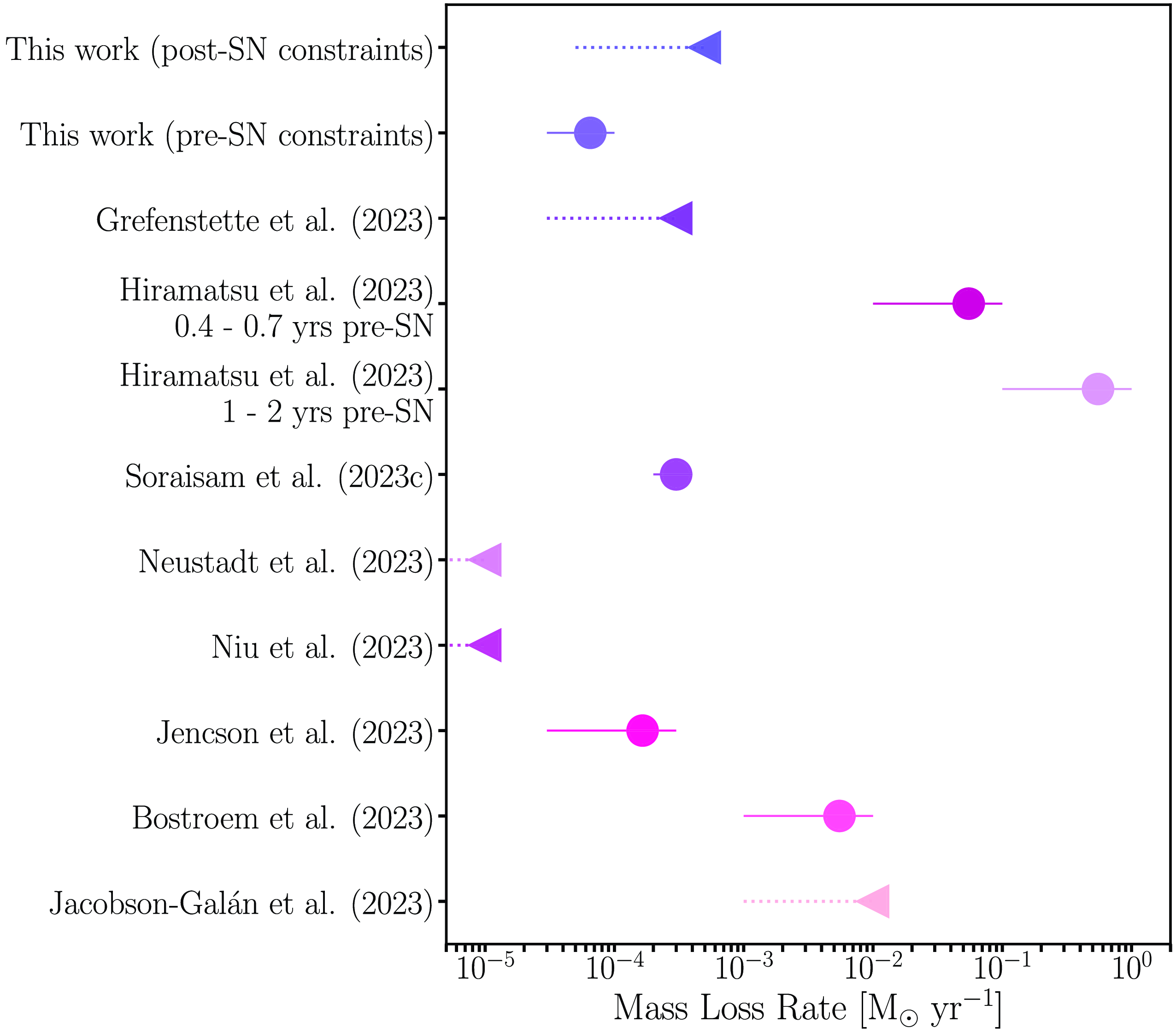
Figure 1. A summary of the mass-loss rates derived from both this study and other studies presented in the literature. Time scales (where available) and methods relevant to each analysis: this work (post-SN): formalism from Margutti et al. (Reference Margutti2012) and Margutti et al. (Reference Margutti2018b),
 $>$
0.5–1.5 yr prior to explosion; this work (pre-SN): mass-loss prescription from Matsumoto & Metzger (Reference Matsumoto and Metzger2022), Grefenstette et al. (Reference Grefenstette, Brightman, Earnshaw, Harrison and Margutti2023): NuSTAR post-explosion (
$>$
0.5–1.5 yr prior to explosion; this work (pre-SN): mass-loss prescription from Matsumoto & Metzger (Reference Matsumoto and Metzger2022), Grefenstette et al. (Reference Grefenstette, Brightman, Earnshaw, Harrison and Margutti2023): NuSTAR post-explosion (
 $t < 11$
days); Hiramatsu et al. (Reference Hiramatsu2023a): numerical light-curve modelling; Soraisam et al. (Reference Soraisam2023c): mass-loss rate prescription from Goldman et al. (Reference Goldman2017), Neustadt et al. (Reference Neustadt, Kochanek and Smith2023): mass-loss prescription from Matsumoto & Metzger (Reference Matsumoto and Metzger2022), Niu et al. (Reference Niu2023): SED modelling and mass-loss prescription from Beasor & Davies (Reference Beasor and Davies2016), Jencson et al. (Reference Jencson2023): SED modelling, 3–19 yr prior to explosion; Bostroem et al. (Reference Bostroem2023): CMFGEN spectral modelling; Jacobson-Galan et al. (Reference Jacobson-Galan2023): light curve and spectral modelling,
$t < 11$
days); Hiramatsu et al. (Reference Hiramatsu2023a): numerical light-curve modelling; Soraisam et al. (Reference Soraisam2023c): mass-loss rate prescription from Goldman et al. (Reference Goldman2017), Neustadt et al. (Reference Neustadt, Kochanek and Smith2023): mass-loss prescription from Matsumoto & Metzger (Reference Matsumoto and Metzger2022), Niu et al. (Reference Niu2023): SED modelling and mass-loss prescription from Beasor & Davies (Reference Beasor and Davies2016), Jencson et al. (Reference Jencson2023): SED modelling, 3–19 yr prior to explosion; Bostroem et al. (Reference Bostroem2023): CMFGEN spectral modelling; Jacobson-Galan et al. (Reference Jacobson-Galan2023): light curve and spectral modelling,
 $\sim$
3–6 yr prior to explosion.
$\sim$
3–6 yr prior to explosion.
From the emergence of a multi-peaked emission line profile of H
 $\alpha$
at
$\alpha$
at
 $t \sim 16$
days, Teja et al. (Reference Teja2023) proposed a shell-shaped CSM with inner and outer radii of
$t \sim 16$
days, Teja et al. (Reference Teja2023) proposed a shell-shaped CSM with inner and outer radii of
 $\sim$
 $8.5\times 10^{14}$
cm and
$8.5\times 10^{14}$
cm and
 $\sim$
 $20.9 \times 10^{14}$
cm, respectively, corresponding to enhanced mass loss
$20.9 \times 10^{14}$
cm, respectively, corresponding to enhanced mass loss
 $\sim$
35–65 yr before the explosion. The flash ionisation features and U–V colour of SN2023ixf led Hiramatsu et al. (Reference Hiramatsu2023a) to suggest a delayed shock breakout due to a dense CSM with a radial extent of
$\sim$
35–65 yr before the explosion. The flash ionisation features and U–V colour of SN2023ixf led Hiramatsu et al. (Reference Hiramatsu2023a) to suggest a delayed shock breakout due to a dense CSM with a radial extent of
 $\sim$
(3–7)
$\sim$
(3–7)
 $\times 10^{14}$
cm. Under the assumption of continuous mass loss, Hiramatsu et al. (Reference Hiramatsu2023a) determined a mass-loss rate of 0.1–1
$\times 10^{14}$
cm. Under the assumption of continuous mass loss, Hiramatsu et al. (Reference Hiramatsu2023a) determined a mass-loss rate of 0.1–1
 $\textrm{M}_\odot \, \textrm{yr}^{-1}$
in the final 1–2 yr before explosion, with the rate decreasing to 0.01–0.1
$\textrm{M}_\odot \, \textrm{yr}^{-1}$
in the final 1–2 yr before explosion, with the rate decreasing to 0.01–0.1
 $\textrm{M}_\odot \, \textrm{yr}^{-1}$
in the
$\textrm{M}_\odot \, \textrm{yr}^{-1}$
in the
 $\sim$
0.4–0.7 yr prior to explosion. Assuming an eruptive mass-loss mechanism, they proposed these eruptions released 0.3–1
$\sim$
0.4–0.7 yr prior to explosion. Assuming an eruptive mass-loss mechanism, they proposed these eruptions released 0.3–1
 $\textrm{M}_\odot$
roughly one year prior to explosion.
$\textrm{M}_\odot$
roughly one year prior to explosion.
Pre-explosion HST and Spitzer images have since revealed a point source at the SN position that is consistent with a RSG progenitor shrouded by a large amount (0.1–1
 $\textrm{M}_\odot$
, Hiramatsu et al. Reference Hiramatsu2023a) of CSM (Soraisam et al. Reference Soraisam2023b,a; Mayya Reference Mayya2023; Jencson et al. Reference Jencson2023; Soraisam et al. Reference Soraisam2023c; Neustadt et al. Reference Neustadt, Kochanek and Smith2023). However, no UV nor X-ray counterpart can be seen in AstroSat-UVIT (Basu et al. Reference Basu, Barway, Anupama, Teja and Dutta2023), Chandra (Kong Reference Kong2023), or XMM-Newton images (Matsunaga et al. Reference Matsunaga, Uchida, Enoto, Tsuru and Sato2023), consistent with our study.
$\textrm{M}_\odot$
, Hiramatsu et al. Reference Hiramatsu2023a) of CSM (Soraisam et al. Reference Soraisam2023b,a; Mayya Reference Mayya2023; Jencson et al. Reference Jencson2023; Soraisam et al. Reference Soraisam2023c; Neustadt et al. Reference Neustadt, Kochanek and Smith2023). However, no UV nor X-ray counterpart can be seen in AstroSat-UVIT (Basu et al. Reference Basu, Barway, Anupama, Teja and Dutta2023), Chandra (Kong Reference Kong2023), or XMM-Newton images (Matsunaga et al. Reference Matsunaga, Uchida, Enoto, Tsuru and Sato2023), consistent with our study.
From the pre-explosion data, progenitor masses of
 $11 \pm 2$
 $\textrm{M}_\odot$
(Kilpatrick et al. Reference Kilpatrick2023),
$\textrm{M}_\odot$
(Kilpatrick et al. Reference Kilpatrick2023),
 $\sim$
12
$\sim$
12
 $\textrm{M}_\odot$
(Pledger & Shara Reference Pledger and Shara2023),
$\textrm{M}_\odot$
(Pledger & Shara Reference Pledger and Shara2023),
 $\sim$
15
$\sim$
15
 $\textrm{M}_\odot$
(Szalai & Dyk Reference Szalai and Dyk2023),
$\textrm{M}_\odot$
(Szalai & Dyk Reference Szalai and Dyk2023),
 $17 \pm 4$
 $\textrm{M}_\odot$
(Jencson et al. Reference Jencson2023),
$\textrm{M}_\odot$
(Jencson et al. Reference Jencson2023),
 $20 \pm 4$
 $ \textrm{M}_\odot$
(Soraisam et al. Reference Soraisam2023c), 16.2–17.4
$ \textrm{M}_\odot$
(Soraisam et al. Reference Soraisam2023c), 16.2–17.4
 $\textrm{M}_\odot$
(Niu et al. Reference Niu2023), and
$\textrm{M}_\odot$
(Niu et al. Reference Niu2023), and
 $\sim$
 $9.3$
–
$9.3$
–
 $13.6$
 $ \textrm{M}_\odot$
(Neustadt et al. Reference Neustadt, Kochanek and Smith2023) have been suggested. In addition, the star formation histories constructed by Niu et al. (Reference Niu2023) using the surrounding resolved stellar populations indicated a higher-mass, Type II SN progenitor in the 17–19
$ \textrm{M}_\odot$
(Neustadt et al. Reference Neustadt, Kochanek and Smith2023) have been suggested. In addition, the star formation histories constructed by Niu et al. (Reference Niu2023) using the surrounding resolved stellar populations indicated a higher-mass, Type II SN progenitor in the 17–19
 $\textrm{M}_{\odot}$
range. Similarly, shock cooling emission models of the light curve indicated a progenitor radius of
$\textrm{M}_{\odot}$
range. Similarly, shock cooling emission models of the light curve indicated a progenitor radius of
 $410 \pm 10$
 $\textrm{R}_{\odot}$
, consistent with a RSG (Hosseinzadeh et al. Reference Hosseinzadeh2023), and in agreement with RSG designations based on HR evolutionary tracks (Kilpatrick et al. Reference Kilpatrick2023; Jencson et al. Reference Jencson2023), the progenitor’s IR colour and pulsations (Soraisam et al. Reference Soraisam2023c), and SED modelling of the progenitor (Neustadt et al. Reference Neustadt, Kochanek and Smith2023).
$\textrm{R}_{\odot}$
, consistent with a RSG (Hosseinzadeh et al. Reference Hosseinzadeh2023), and in agreement with RSG designations based on HR evolutionary tracks (Kilpatrick et al. Reference Kilpatrick2023; Jencson et al. Reference Jencson2023), the progenitor’s IR colour and pulsations (Soraisam et al. Reference Soraisam2023c), and SED modelling of the progenitor (Neustadt et al. Reference Neustadt, Kochanek and Smith2023).
Szalai & Dyk (Reference Szalai and Dyk2023) identified no significant flux variability in pre-explosion Spitzer images collected between 2004 and 2019 that might indicate eruptive mass-loss activity. Likewise, no variability was identified during the progenitor’s final 15 yr using optical pre-explosion data from the Large Binocular Telescope (Neustadt et al. Reference Neustadt, Kochanek and Smith2023), or in pre-explosion ATLAS, ZTF and WISE data (Hiramatsu et al. Reference Hiramatsu2023a). In addition, UV observations from GALEX showed no variability in the 15–20 yr prior to explosion (Flinner et al. Reference Flinner, Tucker, Beacom and Shappee2023). Performing a more detailed analysis of the Spitzer data, Kilpatrick et al. (Reference Kilpatrick2023) identified a 2.8 yr timescale variability in Spitzer 3.6 and 4.6
 $\mu$
m imaging, which was subsequently confirmed by Jencson et al. (Reference Jencson2023) and Soraisam et al. (Reference Soraisam2023c). These authors attributed this variability to pulsations as opposed to an eruptive outburst.
$\mu$
m imaging, which was subsequently confirmed by Jencson et al. (Reference Jencson2023) and Soraisam et al. (Reference Soraisam2023c). These authors attributed this variability to pulsations as opposed to an eruptive outburst.
Searches for pre-explosion optical outbursts in Distance Less Than 40 MPc survey (DLT40), ATLAS, and ZTF data by Dong et al. (Reference Dong2023) found a low probability of significant outbursts in the five years prior to the explosion. They also inferred a maximum ejected CSM mass of
 $\sim0.015 \, \textrm{M}_{\odot}$
, leading them to suggest that if the dense CSM surrounding SN2023ixf is the result of one or more precursor outbursts, they were likely faint, of short duration (
$\sim0.015 \, \textrm{M}_{\odot}$
, leading them to suggest that if the dense CSM surrounding SN2023ixf is the result of one or more precursor outbursts, they were likely faint, of short duration (
 $\sim$
days to months), or occurred more than 5 yr before explosion. Based on their analysis, Dong et al. (Reference Dong2023) proposed that more than one physical mechanism may be responsible for the dense CSM observed in SN2023ixf, such as the interaction of stellar winds from binary companions (e.g. Kochanek Reference Kochanek2019).
$\sim$
days to months), or occurred more than 5 yr before explosion. Based on their analysis, Dong et al. (Reference Dong2023) proposed that more than one physical mechanism may be responsible for the dense CSM observed in SN2023ixf, such as the interaction of stellar winds from binary companions (e.g. Kochanek Reference Kochanek2019).
No emission was initially detected at radio frequencies (Berger et al. Reference Berger2023b; Matthews et al. Reference Matthews2023b; Chandra et al. Reference Chandra, Chevalier, Nayana, Maeda and Ray2023a; Matthews et al. Reference Matthews2023c); however, statistically significant emission with a flux density of
 $41 \pm 8 \,\mu$
Jy was detected 29 days after discovery (Matthews et al. Reference Matthews2023a). Using 1.3 mm (230 GHz) observations, Berger et al. (Reference Berger2023a) determined upper limits of
$41 \pm 8 \,\mu$
Jy was detected 29 days after discovery (Matthews et al. Reference Matthews2023a). Using 1.3 mm (230 GHz) observations, Berger et al. (Reference Berger2023a) determined upper limits of
 $8.6 \times 10^{25} \textrm{erg}\, \textrm{s}^{-1}$
at 2.7 and 7.7 days, and
$8.6 \times 10^{25} \textrm{erg}\, \textrm{s}^{-1}$
at 2.7 and 7.7 days, and
 $3.4 \times 10^{25} \textrm{erg}\, \textrm{s}^{-1}$
at 18.6 days. Searches for neutrinos (Thwaites et al. Reference Thwaites, Vandenbroucke and Santander2023; Nakahata & Super-Kamiokande Collaboration Reference Nakahata2023; Guetta et al. Reference Guetta, Langella, Gagliardini and Della Valle2023) and gamma rays (Marti-Devesa Reference Marti-Devesa2023) from SN2023ixf are consistent with background. Using the derived upper limits from the Fermi-LAT gamma-ray flux and the IceCube neutrino flux, in addition to the shock and CSM properties, Sarmah (Reference Sarmah2023) placed a limit of
$3.4 \times 10^{25} \textrm{erg}\, \textrm{s}^{-1}$
at 18.6 days. Searches for neutrinos (Thwaites et al. Reference Thwaites, Vandenbroucke and Santander2023; Nakahata & Super-Kamiokande Collaboration Reference Nakahata2023; Guetta et al. Reference Guetta, Langella, Gagliardini and Della Valle2023) and gamma rays (Marti-Devesa Reference Marti-Devesa2023) from SN2023ixf are consistent with background. Using the derived upper limits from the Fermi-LAT gamma-ray flux and the IceCube neutrino flux, in addition to the shock and CSM properties, Sarmah (Reference Sarmah2023) placed a limit of
 $\sim10^{-11} \textrm{erg} \, \textrm{cm}^{-2} \, \textrm{s}^{-1}$
on the gamma-ray flux and
$\sim10^{-11} \textrm{erg} \, \textrm{cm}^{-2} \, \textrm{s}^{-1}$
on the gamma-ray flux and
 $\sim10^{-3} \textrm{GeV} \,\textrm{cm}^{-2}$
on the neutrino fluence for emission produced via the proton-proton chain.
$\sim10^{-3} \textrm{GeV} \,\textrm{cm}^{-2}$
on the neutrino fluence for emission produced via the proton-proton chain.
However, X-ray data reveal a point source at the location of SN2023ixf post explosion. NuSTAR observations in the 3–20 keV range show a highly absorbed continuum with a strong emission line at
 $\sim$
 $6.4$
keV, likely attributable to Fe. The extrapolated broadband flux in the 0.3–30 keV range of
$6.4$
keV, likely attributable to Fe. The extrapolated broadband flux in the 0.3–30 keV range of
 $2.3 \times 10^{-12}$
erg cm
$2.3 \times 10^{-12}$
erg cm
 $^{-2}$
s
$^{-2}$
s
 $^{-1}$
yields an intrinsic, absorbed X-ray luminosity of
$^{-1}$
yields an intrinsic, absorbed X-ray luminosity of
 $1.1 \times 10^{40}$
erg s
$1.1 \times 10^{40}$
erg s
 $^{-1}$
(Grefenstette Reference Grefenstette2023). A subsequent detailed analysis of NuSTAR observations yielded an absorbed X-ray luminosity of
$^{-1}$
(Grefenstette Reference Grefenstette2023). A subsequent detailed analysis of NuSTAR observations yielded an absorbed X-ray luminosity of
 $2.5 \times 10^{40}$
erg s
$2.5 \times 10^{40}$
erg s
 $^{-1}$
in the 0.3–79 keV range, assuming a hot, thermal-bremsstrahlung continuum (
$^{-1}$
in the 0.3–79 keV range, assuming a hot, thermal-bremsstrahlung continuum (
 $T > 25$
keV), from which a progenitor mass-loss rate of
$T > 25$
keV), from which a progenitor mass-loss rate of
 $\dot{M} \sim 3 \times 10^{-4}$
 $\textrm{M}_\odot \, \textrm{yr}^{-1}$
was calculated (Grefenstette et al. Reference Grefenstette, Brightman, Earnshaw, Harrison and Margutti2023).
$\textrm{M}_\odot \, \textrm{yr}^{-1}$
was calculated (Grefenstette et al. Reference Grefenstette, Brightman, Earnshaw, Harrison and Margutti2023).
The best-fit model to Chandra observations was found to be a
 $\sim$
10 keV plasma with a column density of
$\sim$
10 keV plasma with a column density of
 $\sim$
 $3.2 \times 10^{22}$
cm
$3.2 \times 10^{22}$
cm
 $^{-2}$
, consistent with a normal stellar wind (Kochanek Reference Kochanek2019). From this, Chandra et al. (Reference Chandra, Maeda, Chevalier, Nayana and Ray2023b) estimated an unabsorbed flux in the 0.3–10 keV band of
$^{-2}$
, consistent with a normal stellar wind (Kochanek Reference Kochanek2019). From this, Chandra et al. (Reference Chandra, Maeda, Chevalier, Nayana and Ray2023b) estimated an unabsorbed flux in the 0.3–10 keV band of
 $(1.6 \pm 0.1) \times 10^{-12}$
erg cm
$(1.6 \pm 0.1) \times 10^{-12}$
erg cm
 $^{-2}$
s
$^{-2}$
s
 $^{-1}$
, corresponding to a luminosity of
$^{-1}$
, corresponding to a luminosity of
 $8 \times 10^{39}$
erg s
$8 \times 10^{39}$
erg s
 $^{-1}$
at a distance of 6.4 Mpc.
$^{-1}$
at a distance of 6.4 Mpc.
Hard X-rays from ART-XC onboard the SRG Observatory were instead found to be best described by an absorbed power-law model with a narrow Gaussian at 6.4 keV and a column density fixed to
 $2 \times 10^{23}$
cm
$2 \times 10^{23}$
cm
 $^{-2}$
. In addition, the ART-XC data showed no variability across a timescale of
$^{-2}$
. In addition, the ART-XC data showed no variability across a timescale of
 $\sim$
10 ks in the 4–12 keV band (Mereminskiy et al. Reference Mereminskiy2023).
$\sim$
10 ks in the 4–12 keV band (Mereminskiy et al. Reference Mereminskiy2023).
Follow-up Swift target-of-opportunity observations identified
 $8.8 \pm 3.7$
background-subtracted counts in a 20-arcsec region around SN2023ixf’s reported position. Assuming an absorbed power law with an index of 1.3 and a column density of
$8.8 \pm 3.7$
background-subtracted counts in a 20-arcsec region around SN2023ixf’s reported position. Assuming an absorbed power law with an index of 1.3 and a column density of
 $2 \times 10^{23}$
cm
$2 \times 10^{23}$
cm
 $^{-2}$
, Kong (Reference Kong2023) found an absorbed flux in the 0.03–30 keV range of
$^{-2}$
, Kong (Reference Kong2023) found an absorbed flux in the 0.03–30 keV range of
 $7.7 \times 10^{-13}$
erg cm
$7.7 \times 10^{-13}$
erg cm
 $^{-2}$
s
$^{-2}$
s
 $^{-1}$
, corresponding to a luminosity of
$^{-1}$
, corresponding to a luminosity of
 $3.8 \times 10^{39}$
erg s
$3.8 \times 10^{39}$
erg s
 $^{-1}$
at 6.4 Mpc. Additionally, Grefenstette et al. (Reference Grefenstette, Brightman, Earnshaw, Harrison and Margutti2023) determined a
$^{-1}$
at 6.4 Mpc. Additionally, Grefenstette et al. (Reference Grefenstette, Brightman, Earnshaw, Harrison and Margutti2023) determined a
 $0.3$
–10 keV flux of
$0.3$
–10 keV flux of
 $6.6^{+10}_{-6.6} \times 10^{-14} \textrm{erg} \,\textrm{cm}^{-2}\,\textrm{s}^{-1}$
using a stacked spectrum consisting of 25 observations spanning 6 days post explosion, a value
$6.6^{+10}_{-6.6} \times 10^{-14} \textrm{erg} \,\textrm{cm}^{-2}\,\textrm{s}^{-1}$
using a stacked spectrum consisting of 25 observations spanning 6 days post explosion, a value
 $\sim$
9 times lower than their result using NuSTAR observations.
$\sim$
9 times lower than their result using NuSTAR observations.
In summary, SN2023ixf is a nearby, interacting, low-luminosity Type II SN from a RSG progenitor that shows signatures of enhanced mass loss during its final years.
3. Observations
SN2023ixf and its progenitor have been extensively observed at multiple wavelengths. In this section, we provide an overview of the UV, optical and X-ray facilities relevant to this study and describe our data reduction and preparation techniques.
3.1 Optical/UV photometry
In Fig. 2, we show the pre-explosion UV/optical light curves of SN2023ixf from the All-Sky Automated Survey for Supernovae (ASAS-SN), the Zwicky Transient Facility (ZTF), the Asteroid Terrestrial-impact Last Alert System (ATLAS), and Swift. In Fig. 3, we show the post-explosion optical/UV light curves of SN2023ixf.
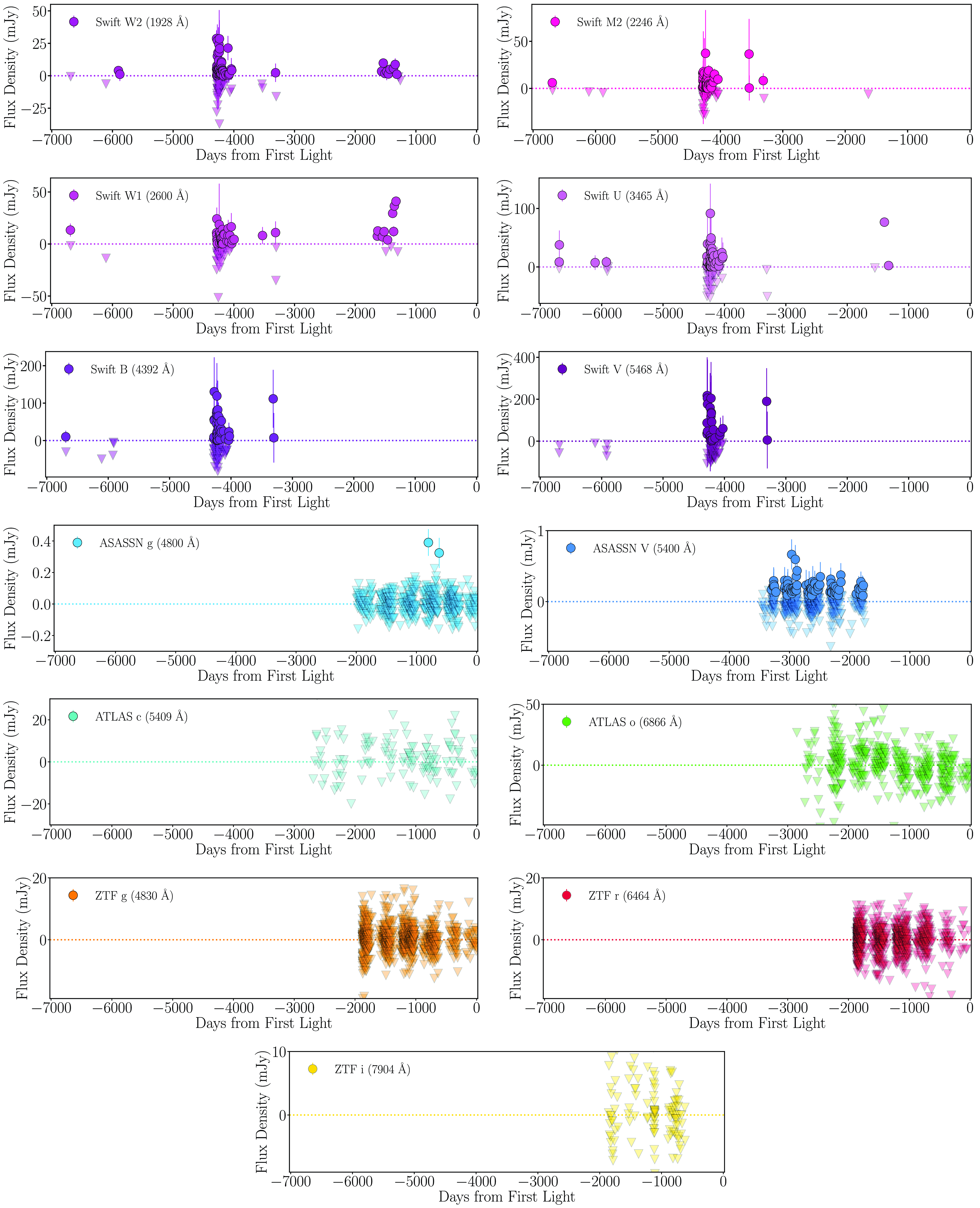
Figure 2. Pre-explosion UV/optical light curves of SN2023ixf as seen by Swift, ASAS-SN, ZTF, and ATLAS. Here, solid data points correspond to fluxes that are
 $\geq3\sigma$
above the reference flux in that band, while the shaded triangles indicate that the emission is consistent with the reference flux in that band.
$\geq3\sigma$
above the reference flux in that band, while the shaded triangles indicate that the emission is consistent with the reference flux in that band.
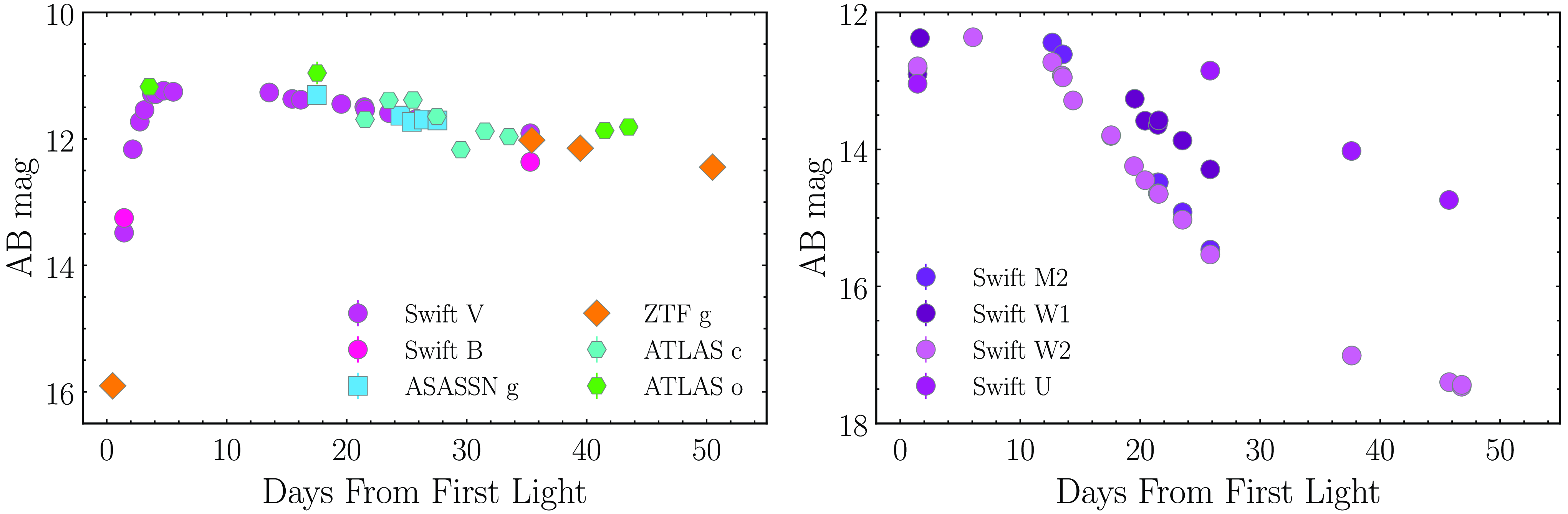
Figure 3. Post-explosion optical (left panel) and UV (right panel) light curves of SN2023ixf as seen by Swift, ASAS-SN, ATLAS, and ZTF. Here, only data detected with
 $\geq3\sigma$
detection significance is shown.
$\geq3\sigma$
detection significance is shown.
3.1.1 ASAS-SN
ASAS-SN (Shappee et al. Reference Shappee2014; Kochanek et al. Reference Kochanek2017; Hart et al. Reference Hart2023) is an automated optical transient survey that monitors the visible sky every
 $\sim$
20 hours to a depth of
$\sim$
20 hours to a depth of
 $\sim$
18.5 mag in the g-band. Starting in late 2011, ASAS-SN began observing the northern sky in the V-band which had a depth of
$\sim$
18.5 mag in the g-band. Starting in late 2011, ASAS-SN began observing the northern sky in the V-band which had a depth of
 $\sim$
17.5 mag. In 2017–2018, the survey switched to the g-band to gain a magnitude of depth and added additional units for cadence. The survey now consists of 20 individual telescopes with 14-cm aperture Nikon telephoto lenses with
$\sim$
17.5 mag. In 2017–2018, the survey switched to the g-band to gain a magnitude of depth and added additional units for cadence. The survey now consists of 20 individual telescopes with 14-cm aperture Nikon telephoto lenses with
 $\sim$
8 arcsec pixels that are grouped together into five 4-telescope units. The five telescope units are located at Haleakala Observatory, McDonald Observatory, the South African Astrophysical Observatory, with the remaining two at the Cerro Tololo Inter-American Observatory.
$\sim$
8 arcsec pixels that are grouped together into five 4-telescope units. The five telescope units are located at Haleakala Observatory, McDonald Observatory, the South African Astrophysical Observatory, with the remaining two at the Cerro Tololo Inter-American Observatory.
We used the Sky Patrol V1Footnote
a
(Kochanek et al. Reference Kochanek2017) to to obtain image-subtracted light curves for the location of SN2023ixf in addition to a grid of 13 points adjacent to the SN location. The Sky Patrol uses images reduced by the ASAS-SN fully automated pipeline which includes the ISIS image subtraction package (Alard & Lupton Reference Alard and Lupton1998; Alard Reference Alard2000). When serving image-subtracted light curves, the Sky Patrol first co-adds the subtracted images from the 3 dithers taken at each pointing during survey operations. To derive the g- and V-band photometry from these images, Sky Patrol V1 uses the IRAF apphot package with a 2-pixel (or
 $\sim$
16 arcsec) radius aperture to perform aperture photometry on each subtracted image, generating a differential light curve. The photometry is calibrated using the AAVSO Photometric All-Sky Survey (Henden et al. Reference Henden, Levine, Terrell and Welch2015). Images with a full width at half maximum of 1.7 pixels or greater and images with a shallow depth (3
$\sim$
16 arcsec) radius aperture to perform aperture photometry on each subtracted image, generating a differential light curve. The photometry is calibrated using the AAVSO Photometric All-Sky Survey (Henden et al. Reference Henden, Levine, Terrell and Welch2015). Images with a full width at half maximum of 1.7 pixels or greater and images with a shallow depth (3
 $\sigma$
detection limit of
$\sigma$
detection limit of
 $<$
18.4 mag) were discarded. ASAS-SN observed M101 665 times from Jan 2012 to Nov 2018 in the V-band and 864 times from Nov 2017 through May 2023 in the g-band.
$<$
18.4 mag) were discarded. ASAS-SN observed M101 665 times from Jan 2012 to Nov 2018 in the V-band and 864 times from Nov 2017 through May 2023 in the g-band.
3.1.2 ATLAS
ATLAS currently consists of a quadruple 0.5-m telescope system that has two units in Hawaii (Haleakala and Mauna Loa), one in Chile (El Sauce), and one in South Africa (Sutherland). The ATLAS observing strategy is to obtain a sequence of four 30-s exposures spread out over an hour (Smith et al. Reference Smith2020), using either a cyan (c) filter [4,420–650 nm] or an orange (o) filter [560–820 nm], depending on the Moon phase (Tonry et al. Reference Tonry2018a). The pixel scale of ATLAS is
 $\sim$
 $1.9$
arcsec/pixel and the typical PSF is
$1.9$
arcsec/pixel and the typical PSF is
 $\sim$
4 arcsec.
$\sim$
4 arcsec.
ATLAS data are accessible through the ATLAS Forced Photometry ServerFootnote b (Shingles et al. Reference Shingles2021). The photometric routine used, called tphot, is based on algorithms described in Tonry (Reference Tonry2011) and Sonnett et al. (Reference Sonnett2013) and can be deployed on either reduced or difference images. Both types of images have been calibrated astrometrically and photometrically using the ATLAS All-Sky Stellar Reference Catalog (Refcat, Tonry et al. Reference Tonry2018b), and the difference images also use a modified version of the image subtraction algorithm HOTPANTS (Becker Reference Becker2015) to subtract a reference sky frame.
Counting each 30-s exposure individually, ATLAS has observed the location of SN2023ixf 2491 times between 30 July 2015 and 2 July 2023. We do not use photometry from images where the location of SN2023ixf is within 40 pixels of a chip edge (10 images), where the best-fit axis ratio of a source at that location is above 1.5 (16 images), where the
 $5\sigma$
limiting magnitude is less than 16 (56 images), or where the ATLAS pipeline presents an error flag (no images). This leaves us with 1 844 o-band and 548 c-band images.
$5\sigma$
limiting magnitude is less than 16 (56 images), or where the ATLAS pipeline presents an error flag (no images). This leaves us with 1 844 o-band and 548 c-band images.
We then co-added nightly observations, discarding observations with flux values over three times their uncertainty from the median flux, weighting the remaining observations by their inverse variance in flux, and recording the interpolated 50th percentile values for epoch, flux, and uncertainty. The final light curve has 438 o-band entries and 123 c-band entries.
3.1.3 Zwicky transient facility
ZTF g-, r-, and i-band photometry covering the full ZTF survey from 17 March 2018 (
 $\textrm{JD}=2\,458\,194.5$
) until 08 July 2023 (
$\textrm{JD}=2\,458\,194.5$
) until 08 July 2023 (
 $\textrm{JD}=2460133.8$
) were obtained using the ZTF forced photometry service (Masci et al. Reference Masci2019). This covers a phase of
$\textrm{JD}=2460133.8$
) were obtained using the ZTF forced photometry service (Masci et al. Reference Masci2019). This covers a phase of
 $\sim$
 $1\,850$
days prior to discovery until
$1\,850$
days prior to discovery until
 $\sim$
50 days after discovery of SN2023ixf. Following the procedure outlined in the ZTF forced photometry manual v2.3,Footnote
c
we apply the standard baseline corrections to the data and use a signal-to-noise threshold of 3 for all available data. We note that ZTF has a characteristic pixel scale of
$\sim$
50 days after discovery of SN2023ixf. Following the procedure outlined in the ZTF forced photometry manual v2.3,Footnote
c
we apply the standard baseline corrections to the data and use a signal-to-noise threshold of 3 for all available data. We note that ZTF has a characteristic pixel scale of
 $\sim1$
arcsec/pixel and a PSF of
$\sim1$
arcsec/pixel and a PSF of
 $\sim2$
arcsec.
$\sim2$
arcsec.
3.1.4 Swift UVOT
Due to its proximity and the discovery of SN2011fe in 2011, M101 has been extensively monitored by Swift. Prior to the discovery of SN2023ixf, there had been 218 observations overlapping the location of this event. These observations were carried out between 29 August 2006 (
 $\textrm{M}JD=53976.48613$
) and 08 December 2019
$\textrm{M}JD=53976.48613$
) and 08 December 2019
 $(\textrm{MJD=58825.72311}$
) and have Swift target IDs of 35892, 30896, 32081, 32088, 32094, 32101, 33635, 11002, and 32481. These observations were conducted using both the UltraViolet and Optical Telescope (Roming et al. Reference Roming2005, UVOT) and the X-ray Telescope (Burrows et al. Reference Burrows2005, XRT). The total exposure time of these observations is
$(\textrm{MJD=58825.72311}$
) and have Swift target IDs of 35892, 30896, 32081, 32088, 32094, 32101, 33635, 11002, and 32481. These observations were conducted using both the UltraViolet and Optical Telescope (Roming et al. Reference Roming2005, UVOT) and the X-ray Telescope (Burrows et al. Reference Burrows2005, XRT). The total exposure time of these observations is
 $\sim$
431 ks.
$\sim$
431 ks.
Since the discovery of SN2023ixf until September 2023, Swift has observed the source 58 times. These observations began on 20 May 2023 (
 $\textrm{M}JD=60\,084.26901$
) and have Swift target IDs of 16038, 16043, 32481, and 89625. The total combined exposure of these observations is
$\textrm{M}JD=60\,084.26901$
) and have Swift target IDs of 16038, 16043, 32481, and 89625. The total combined exposure of these observations is
 $\sim$
68 ks. For the majority of Swift observations, Swift observed either SN2023ixf or the location of the SN using at least one or more of the six UVOT filters (Poole et al. Reference Poole2008: V (5 425.3 Å), B (4 349.6 Å), U (3 467.1 Å), UVW1 (2 580.8 Å), UVM2 (2 246.4 Å), and UVW2 (2 054.6 Å)).
$\sim$
68 ks. For the majority of Swift observations, Swift observed either SN2023ixf or the location of the SN using at least one or more of the six UVOT filters (Poole et al. Reference Poole2008: V (5 425.3 Å), B (4 349.6 Å), U (3 467.1 Å), UVW1 (2 580.8 Å), UVM2 (2 246.4 Å), and UVW2 (2 054.6 Å)).
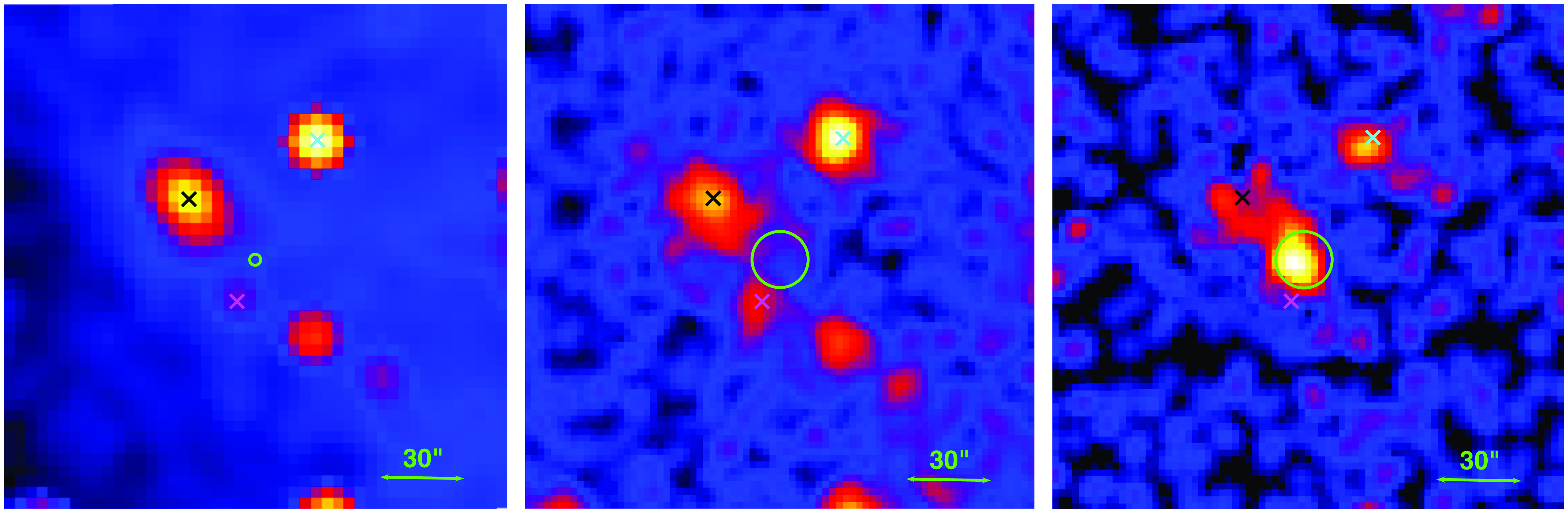
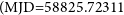
Figure 4. (Left Panel): The merged, broadband, pre-explosion Chandra observation of the location of SN2023ixf. The two arcsecond radius green circle shows the location of SN2023ixf, and the black, cyan, and magenta crosses mark the locations of the high-mass X-ray binaries (HMXBs) CXO J140341.1+541903, CXO J140336.1+541924, and [CHP2004] J140339.3+541827, respectively. (Middle Panel): The merged, broadband Swift observation obtained using all available pre-explosion observations. The green circle here has a radius of 15 arcsec and is centered on SN2023ixf used to derive count rates. (Right panel:) The merged, broadband Swift observation created using all available post-explosion observations. Here the green circle has a 20 arcsec radius and is centered on SN2023ixf. Significant X-ray emission arises from the location of the source. Note that the images are all aligned to a common reference frame.
To derive the UVOT photometry both prior to and during the rise of SN2023ixf, we used the HEASARC uvotsource package. To extract the UV and optical counts, we used a circular region with a 5-arcsec radius centered on the position of SN2023ixf and source-free background regions with a radius of 20 arcsec located at (
 $\alpha$
,
$\alpha$
,
 $\delta$
) = (14:03:42.5088, +54:18:12.172) and (
$\delta$
) = (14:03:42.5088, +54:18:12.172) and (
 $\alpha$
,
$\alpha$
,
 $\delta$
) = (14:03:31.6839, +54:16:03.572) for the pre- and post-discovery data, respectively. Similar to Hosseinzadeh et al. (Reference Hosseinzadeh2023), we find that the majority of the early post-explosion Swift UVOT observations were saturated due to the high count rate of the source and thus we discard these data and only use those that are below the maximum countrate limit of the UVOT detector. The UVOT count rates are converted into AB magnitudes and flux densities using the most recent calibrations (Poole et al. Reference Poole2008; Breeveld et al. Reference Breeveld2010). We do not correct the photometry for Galactic extinction.
$\delta$
) = (14:03:31.6839, +54:16:03.572) for the pre- and post-discovery data, respectively. Similar to Hosseinzadeh et al. (Reference Hosseinzadeh2023), we find that the majority of the early post-explosion Swift UVOT observations were saturated due to the high count rate of the source and thus we discard these data and only use those that are below the maximum countrate limit of the UVOT detector. The UVOT count rates are converted into AB magnitudes and flux densities using the most recent calibrations (Poole et al. Reference Poole2008; Breeveld et al. Reference Breeveld2010). We do not correct the photometry for Galactic extinction.
3.2 X-ray observations
3.2.1 Swift XRT
In addition to the UVOT, Swift simultaneously observed the location and rise of SN2023ixf using the XRT in photon-counting mode. Following the Swift XRT reduction guide, we reduced all observations using the standard filter and screening criteria, and the most up-to-date calibration files. Using the task XRTPIPELINE, we reprocessed all level one XRT data, producing cleaned event files and exposure maps for all observations.
To increase the signal-to-noise ratio of our observations, we combined our individual images using XSELECT version 2.5b. Here, we combined the observations taken prior to the discovery of SN2023ixf into 33 time bins, spanning
 $\sim$
 $6\,000$
days since the first serendipitous Swift observation of this location. For the observations taken post-discovery, we combined these observations into 19 time bins spanning
$6\,000$
days since the first serendipitous Swift observation of this location. For the observations taken post-discovery, we combined these observations into 19 time bins spanning
 $\sim$
46 days after first light. We also merged all observations taken prior to and after the discovery of SN2023ixf to produce a deep Swift XRT observation for both before and after the discovery of SN2023ixf (see Fig. 4 middle and right panel).
$\sim$
46 days after first light. We also merged all observations taken prior to and after the discovery of SN2023ixf to produce a deep Swift XRT observation for both before and after the discovery of SN2023ixf (see Fig. 4 middle and right panel).
Background-subtracted count rates were derived from each of these merged observations using a 20 arcsec source region centered on the position of SN2023ixf for observations taken after discovery and a 15-arcsec source region for observations taken prior to discovery. A smaller source region was used for the pre-explosion observations due to the presence of an X-ray bright source near the location of SN2023ixf in both the deep Chandra and Swift images that were obtained by merging all available observations taken prior to peak (see Fig. 4 left and middle panel). However, as these sources were only observable in these deep exposures and were not seen in the individual observations taken post-explosion due to the brightness of SN2023ixf, we use a larger region to maximise the flux from this event. The total exposure time of these merged observations was 431.2 and 68 ks, for the pre- and post-explosion observations, respectively. For all observations we used the same source-free background region with a radius of 100 arcsec centered at
 $(\alpha,\delta)$
= (14:03:27.7541, +54:14:16.237). This region, as well as the background regions used for the Chandra and XMM-Newton observations, were selected to capture the local diffuse emission and background contribution. All extracted count rates were corrected for the encircled energy fraction (Moretti et al. Reference Flanagan and Siegmund2004).
$(\alpha,\delta)$
= (14:03:27.7541, +54:14:16.237). This region, as well as the background regions used for the Chandra and XMM-Newton observations, were selected to capture the local diffuse emission and background contribution. All extracted count rates were corrected for the encircled energy fraction (Moretti et al. Reference Flanagan and Siegmund2004).
Using our merged event files, we extracted a spectrum from the position of the source using the Swift analysis tool XRTPRODUCTS and the source and background regions defined above. Ancillary response files were generated using the task XRTMKARF and the individual exposure maps from xrtpipeline that were merged using the HEASARC analysis tool ximage version 4.5.1. The response matrix files were obtained from the most recent calibration database. The resulting spectrum was grouped to have a minimum of 15 counts per energy bin using the ftools command grppha.
3.2.2 Chandra
The location of SN2023ixf has been serendipitously observed using the Chandra X-ray Observatory 21 times since 2000, with the most recent archival observation taken in 2017. These observations were taken in VFAINT or FAINT mode under the observation IDs: 934, 6175, 6170, 6169, 6152, 6118, 6115, 6114, 5323, 5322, 5309, 5300, 5297, 5296, 4737, 4736, 4735, 4733, 4732, 4731, 2065, and 19304. These observations were conducted using the ACIS-S detector and have a total combined exposure time of
 $\sim$
966.2 ks.
$\sim$
966.2 ks.
All Chandra data were reduced using version 4.15 of the Chandra analysis software CIAO. We reprocessed the level one data using the CIAO command chandra_repro and the most up-to-date calibration database. To improve the absolute astrometry of these observations, we used the CIAO tool wcs_match and cross-matched X-ray sources found within these observations using the tool wavdetect, with the USNO-A2.0 catalog.Footnote d We then used reproject_obs to reproject these event files to a common tangent point based on the updated world coordinate system (WCS) information of the earliest and deepest Chandra observation in our dataset (ObsID: 934). This command also takes the reprojected event files and merges them together to form a single event file. We then used flux_obs to combine the reprojected observations to create an exposure-corrected image in the broad (see Fig. 4 left panel), soft, medium, and hard energy bands (see Fig. 5).
Figure 5. A merged and exposure-corrected Chandra X-ray image of the location of SN2023ixf (green diamond). The black, cyan, and magenta crosses mark the locations of HMXBs CXO J140341.1+541903, CXO J140336.1+541924, and [CHP2004] J140339.3+541827, respectively. Here, the 0.5–1.2 keV (soft) emission is in red, the 1.2–2.0 keV (medium) emission is in green, and the 2.0–7.0 keV (hard) emission is in blue.
To place constraints on pre-explosion X-ray emission, we used a circular region centered on SN2023ixf with a radius of 2 arcsec and a source-free, local, background region located at
 $(\alpha,\delta)$
= (14:03:27.4629, +54:17:34.929) with a radius of 20 arcsec. A region of this size encloses 95% of all source photons at 1.496 keV, and as such, the extracted count rates were corrected for encircled energy fraction.Footnote
e
$(\alpha,\delta)$
= (14:03:27.4629, +54:17:34.929) with a radius of 20 arcsec. A region of this size encloses 95% of all source photons at 1.496 keV, and as such, the extracted count rates were corrected for encircled energy fraction.Footnote
e
3.2.3 XMM-Newton
XMM-Newton observed the location of SN2023ixf four times prior to its explosion. The first observation was taken in 2002, with the most recent from 2018. These observations have ObsIDs 0104260101, 0164560701, 0212480201, and 0824450501, totaling
 $\sim$
 $220\,$
ks prior to filtering. To analyse these observations, we used the XMM-Newton Science System (SAS) version 20.0.0 and the most up-to-date calibration file. Before extracting count rates, we produced cleaned event files by removing time intervals which were contaminated by a high background, or those during which proton flares were identified when generating count rate histograms for energies between 10.0–12.0 keV. We used the standard screening criteria as suggested by the current SAS analysis threads and XMM-Newton Users Handbook. For the MOS detectors, we used single to quadruple patterned events (PATTERN
$220\,$
ks prior to filtering. To analyse these observations, we used the XMM-Newton Science System (SAS) version 20.0.0 and the most up-to-date calibration file. Before extracting count rates, we produced cleaned event files by removing time intervals which were contaminated by a high background, or those during which proton flares were identified when generating count rate histograms for energies between 10.0–12.0 keV. We used the standard screening criteria as suggested by the current SAS analysis threads and XMM-Newton Users Handbook. For the MOS detectors, we used single to quadruple patterned events (PATTERN
 $\leq$
12), while for the PN detectors only single and double patterned events (PATTERN
$\leq$
12), while for the PN detectors only single and double patterned events (PATTERN
 $\leq$
4) were selected. The standard canned screening set of FLAGS for both the MOS (#XMMEA_EM) and PN (#XMMEA_EP) detector were also selected.
$\leq$
4) were selected. The standard canned screening set of FLAGS for both the MOS (#XMMEA_EM) and PN (#XMMEA_EP) detector were also selected.
Count rates were extracted from a circular region with a radius of 20 arcsec centered on the location of SN2023ixf and a source-free, local, background region of radius 90 arcsec centered at
 $(\alpha,\delta)$
= (14:03:40.1033, +54:21:13.639). As a region of this size encloses only
$(\alpha,\delta)$
= (14:03:40.1033, +54:21:13.639). As a region of this size encloses only
 $\sim$
80% of all source photons, all extracted counts were corrected for this aperture. Before extracting our counts, we combined both the MOS and PN detectors for each observation using the SAS tools command merge.
$\sim$
80% of all source photons, all extracted counts were corrected for this aperture. Before extracting our counts, we combined both the MOS and PN detectors for each observation using the SAS tools command merge.
4. Analysis
In this section, we infer the properties of the progenitor of SN2023ixf by searching for evidence of pre-explosion variability and mass loss using both pre- and post-explosion observations.
4.1 Properties of the explosion
To constrain the pre-explosion mass loss using post-explosion X-ray observations (see Section 5.2.2), we require an estimate of the bolometric luminosity. As such, we use the SUPERBOL pipeline (Nicholl Reference Nicholl2018) to calculate the bolometric light curve using the Swift UVOT light curves extracted post-explosion and the u/U, B, g, V, r/R, i/I, and z photometry published in Figure 1 of Jacobson-Galan et al. (Reference Jacobson-Galan2023). To show all light curves across the same timescale, we used the i-band as the reference filter and interpolated/extrapolated each light curve using a polynomial of order four between MJD 60082 and MJD 60100. We also assume a host reddening to SN 2023ixf of E(B – V) = 0.033 mag from Jacobson-Galan et al. (Reference Jacobson-Galan2023) that was derived from NaI D line absorption from the optical spectra of this event. We then fit the resulting SED with a blackbody model to derive the luminosity, radius, and temperature. In Fig. 6, we present our derived bolometric luminosity for SN2023ixf, along with the bolometric luminosities of other Type IIn SNe and the pseudobolometric luminosity for SN2023ixf from Hiramatsu et al. (Reference Hiramatsu2023a).
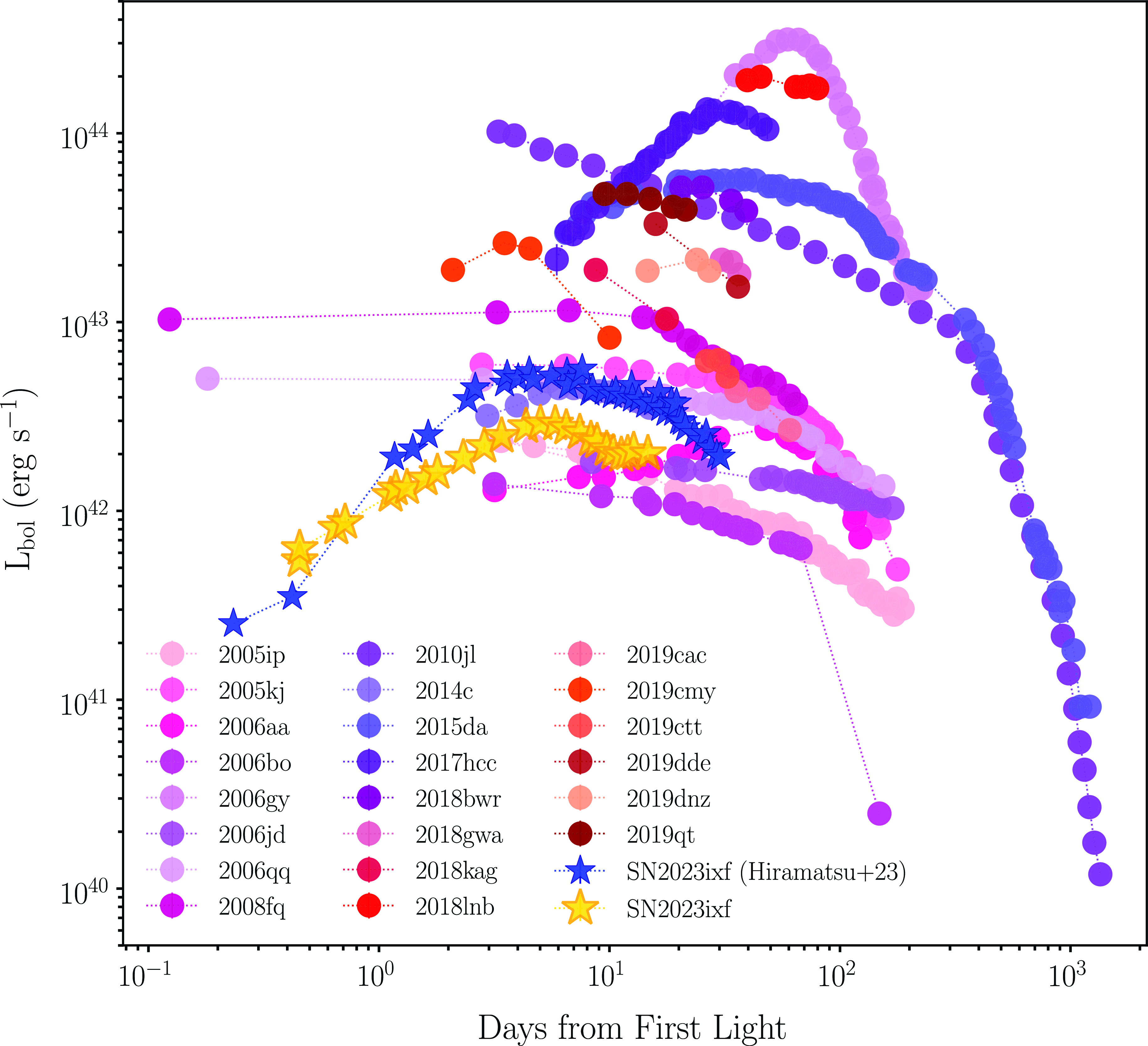
Figure 6. The bolometric light curve of SN2023ixf (yellow stars) compared to the pseudobolometric light curve (UBVRI, blue stars) from Hiramatsu et al. (Reference Hiramatsu2023a) and a sample of other Type IIn SNe. Data Sources: SN2006gy (Smith et al. Reference Smith, Chornock, Silverman, Filippenko and Foley2010); SN2010jl (Chandra et al. Reference Chandra, Chevalier, Chugai, Fransson and Soderberg2015); SN2014c (Margutti et al. Reference Margutti2017); SN2015da (Tartaglia et al. Reference Tartaglia2020); SN2017hcc (Prieto et al. Reference Prieto2017); SNe 2018bwr, 2018gwa, 2018kag, 2018lnb, 2019cac, 2019cmy, 2019ctt, 2019dde, 2019dnz, 2019qt (Soumagnac et al. Reference Soumagnac2020); and all remaining SNe (Taddia et al. Reference Taddia2013).
Our analysis in Section 5.2.2 also requires an estimate of the ejecta mass. From the analytical light curve model of Hiramatsu et al. (Reference Hiramatsu2023b) that attributes the SN emission to shock interaction between the ejecta and the CSM, we use
 $\nu=\sqrt{\frac{2(5-\delta)(n-5)E_{SN}}{(3-\delta)(n-3)M_{SN}}}$
to estimate the ejecta mass. Here,
$\nu=\sqrt{\frac{2(5-\delta)(n-5)E_{SN}}{(3-\delta)(n-3)M_{SN}}}$
to estimate the ejecta mass. Here,
 $M_{SN}$
is the ejecta mass,
$M_{SN}$
is the ejecta mass,
 $E_{SN}$
is the explosion energy, the exponents of the broken power law that describes the density of the unshocked SN ejecta are
$E_{SN}$
is the explosion energy, the exponents of the broken power law that describes the density of the unshocked SN ejecta are
 $\delta=0$
and
$\delta=0$
and
 $n=12$
(as is standard for RSG progenitors), and
$n=12$
(as is standard for RSG progenitors), and
 $\nu$
is the characteristic velocity of the ejecta which corresponds to the photospheric velocity at maximum light (see Equation 4 from Hiramatsu et al. Reference Hiramatsu2023b). For
$\nu$
is the characteristic velocity of the ejecta which corresponds to the photospheric velocity at maximum light (see Equation 4 from Hiramatsu et al. Reference Hiramatsu2023b). For
 $\nu$
, we use the lower limit on the SN shock velocity from Jacobson-Galan et al. (Reference Jacobson-Galan2023), who determined a value of 8 500 km s
$\nu$
, we use the lower limit on the SN shock velocity from Jacobson-Galan et al. (Reference Jacobson-Galan2023), who determined a value of 8 500 km s
 $^{-1}$
using the blue edge of the H
$^{-1}$
using the blue edge of the H
 $\alpha$
absorption profile. Assuming
$\alpha$
absorption profile. Assuming
 $E_{SN}=(0.5-2)\times10^{51}$
erg s
$E_{SN}=(0.5-2)\times10^{51}$
erg s
 $^{-1}$
, we get an ejecta mass of 0.9–3.6
$^{-1}$
, we get an ejecta mass of 0.9–3.6
 $\textrm{M}_{\odot}$
, with an energy of
$\textrm{M}_{\odot}$
, with an energy of
 $E_{SN}=10^{51}$
erg s
$E_{SN}=10^{51}$
erg s
 $^{-1}$
corresponding to an ejecta mass of
$^{-1}$
corresponding to an ejecta mass of
 $1.8\, \textrm{M}_{\odot}$
.
$1.8\, \textrm{M}_{\odot}$
.
4.2 Variability
To constrain the presence of variability prior to explosion, we take advantage of the methods presented in Johnson et al. (Reference Johnson, Kochanek and Adams2017, Reference Johnson, Kochanek and Adams2018) and Neustadt et al. (Reference Neustadt, Kochanek and Smith2023). Here, we examine the variability of the progenitor by calculating the peak-to-peak luminosity changes of the pre-SN differential light curves (
 $\Delta\lambda L_{\lambda}$
). We then compare this variability to both the root mean square (RMS) of our data and to the RMS scatter of the comparison sample about the mean of their peak-to-peak luminosity changes. Our comparison sample consists of regions nearby the position of the SN from which these comparison light curves were extracted. This was done to better understand any systematic errors in the light curves. For our Swift and ZTF sample, we used a total of 12 control light curves, while for ATLAS and ASAS-SN we used 7 and 13, respectively. These sample points were chosen to avoid obvious nearby sources such as the optical/UV bright HMXBs shown in Figs. 4 and 5.
$\Delta\lambda L_{\lambda}$
). We then compare this variability to both the root mean square (RMS) of our data and to the RMS scatter of the comparison sample about the mean of their peak-to-peak luminosity changes. Our comparison sample consists of regions nearby the position of the SN from which these comparison light curves were extracted. This was done to better understand any systematic errors in the light curves. For our Swift and ZTF sample, we used a total of 12 control light curves, while for ATLAS and ASAS-SN we used 7 and 13, respectively. These sample points were chosen to avoid obvious nearby sources such as the optical/UV bright HMXBs shown in Figs. 4 and 5.
In Figs. 7–10, we present our resulting peak-to-peak luminosity variability analysis for both the progenitor of SN2023ixf and our control light curves.
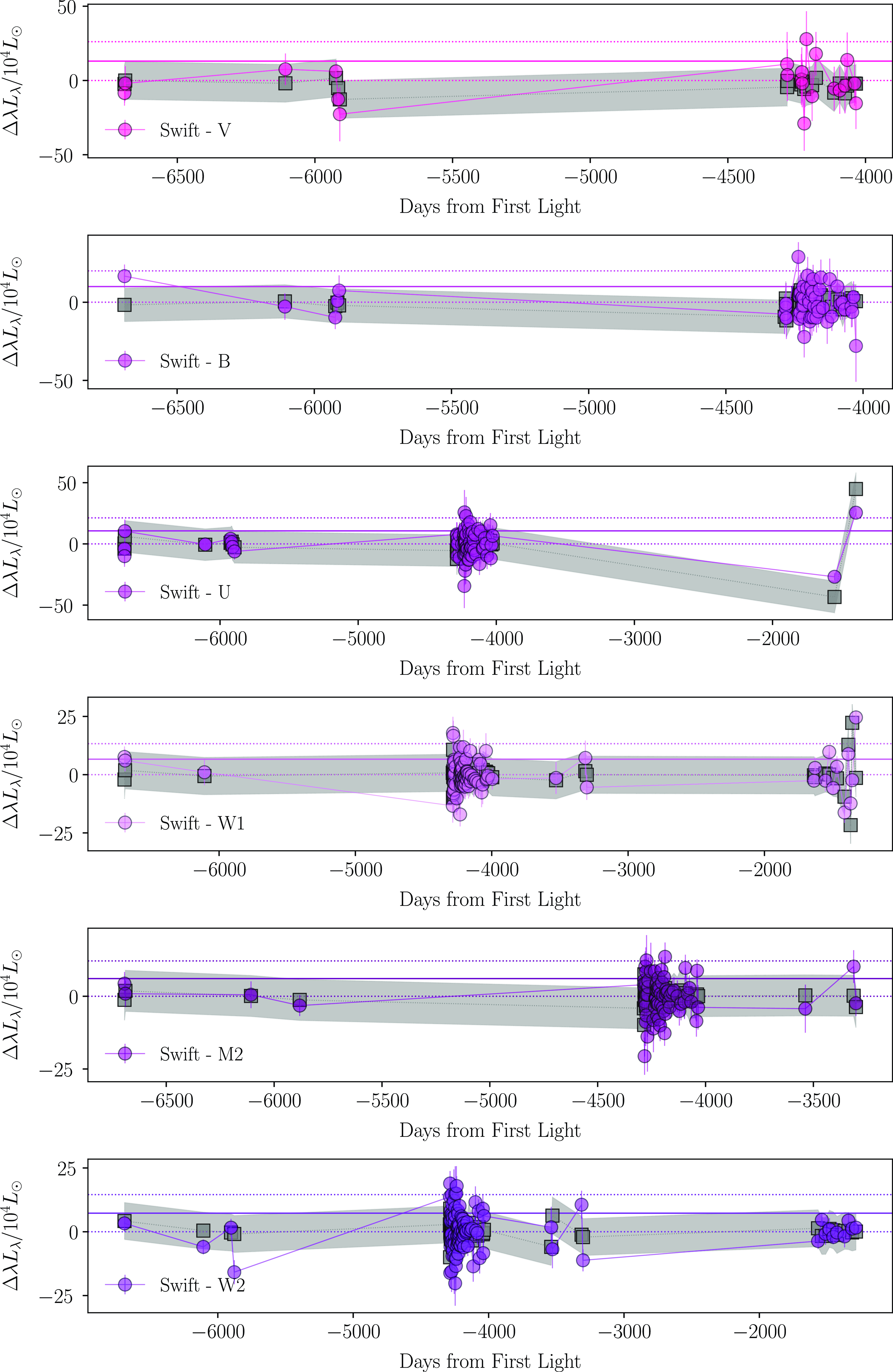
Figure 7. The peak-to-peak luminosity changes of the pre-SN differential luminosity (
 $\Delta\lambda L_{\lambda}$
) of the SN2023ixf progenitor as observed in the Swift UVOT filters (solid coloured circles). The solid horizontal lines correspond to the root mean square of the peak-to-peak luminosity of our pre-explosion light curves, while the dotted lines correspond to the 1
$\Delta\lambda L_{\lambda}$
) of the SN2023ixf progenitor as observed in the Swift UVOT filters (solid coloured circles). The solid horizontal lines correspond to the root mean square of the peak-to-peak luminosity of our pre-explosion light curves, while the dotted lines correspond to the 1
 $\sigma$
scatter. The grey squares correspond to the mean of the peak-to-peak luminosity changes of our comparison sample, while the shaded grey regions correspond to the standard deviation of this mean. The observed scatter in the luminosity of SN2023ixf’s progenitor is consistent with the comparison sample, indicating no pre-SN variability of SN2023ixf at these wavelengths.
$\sigma$
scatter. The grey squares correspond to the mean of the peak-to-peak luminosity changes of our comparison sample, while the shaded grey regions correspond to the standard deviation of this mean. The observed scatter in the luminosity of SN2023ixf’s progenitor is consistent with the comparison sample, indicating no pre-SN variability of SN2023ixf at these wavelengths.
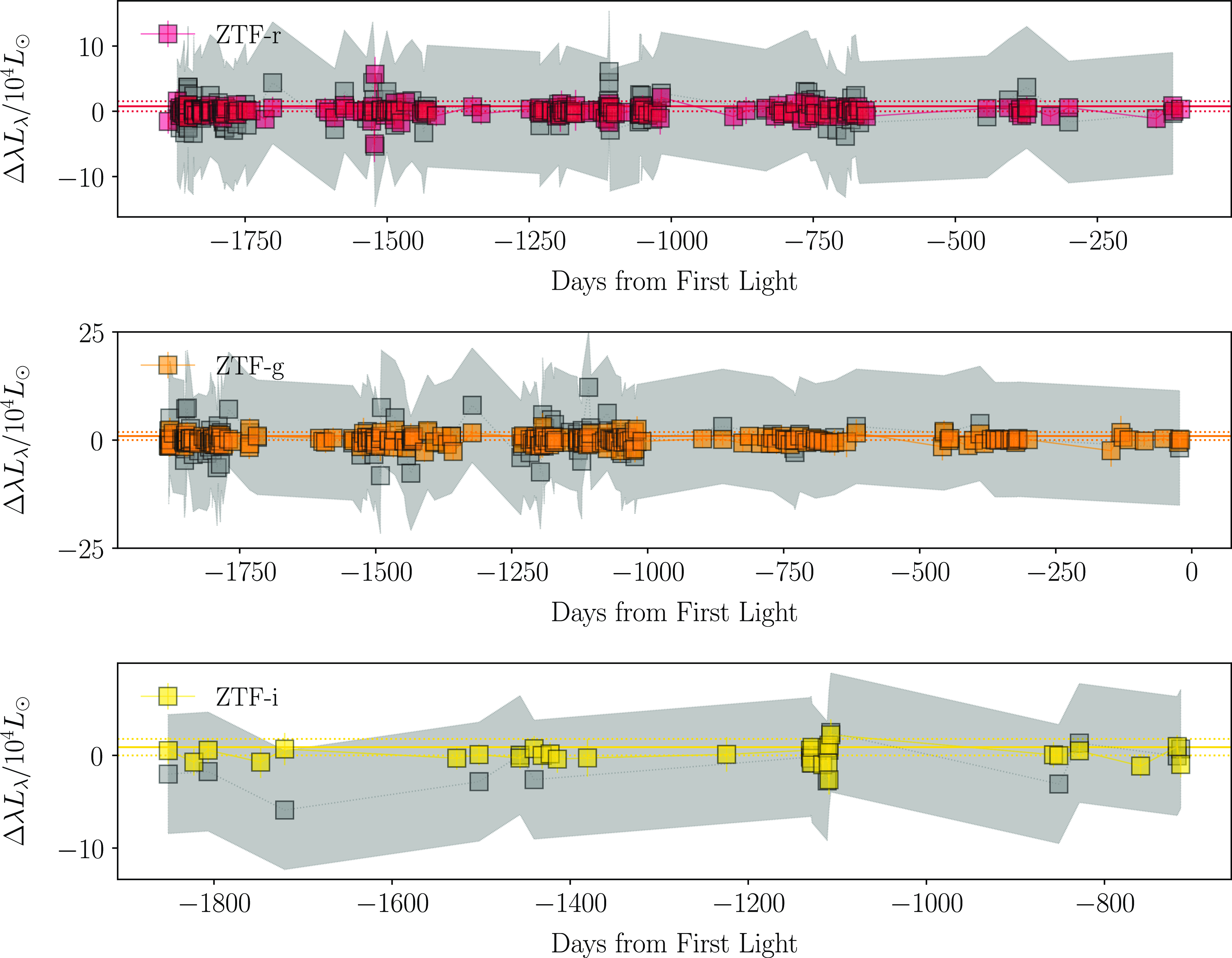
Figure 8. The peak-to-peak luminosity changes of the pre-SN differential luminosity (
 $\Delta\lambda L_{\lambda}$
) of the SN2023ixf progenitor as observed in the ZTF filters. See Fig. 7 for more details.
$\Delta\lambda L_{\lambda}$
) of the SN2023ixf progenitor as observed in the ZTF filters. See Fig. 7 for more details.
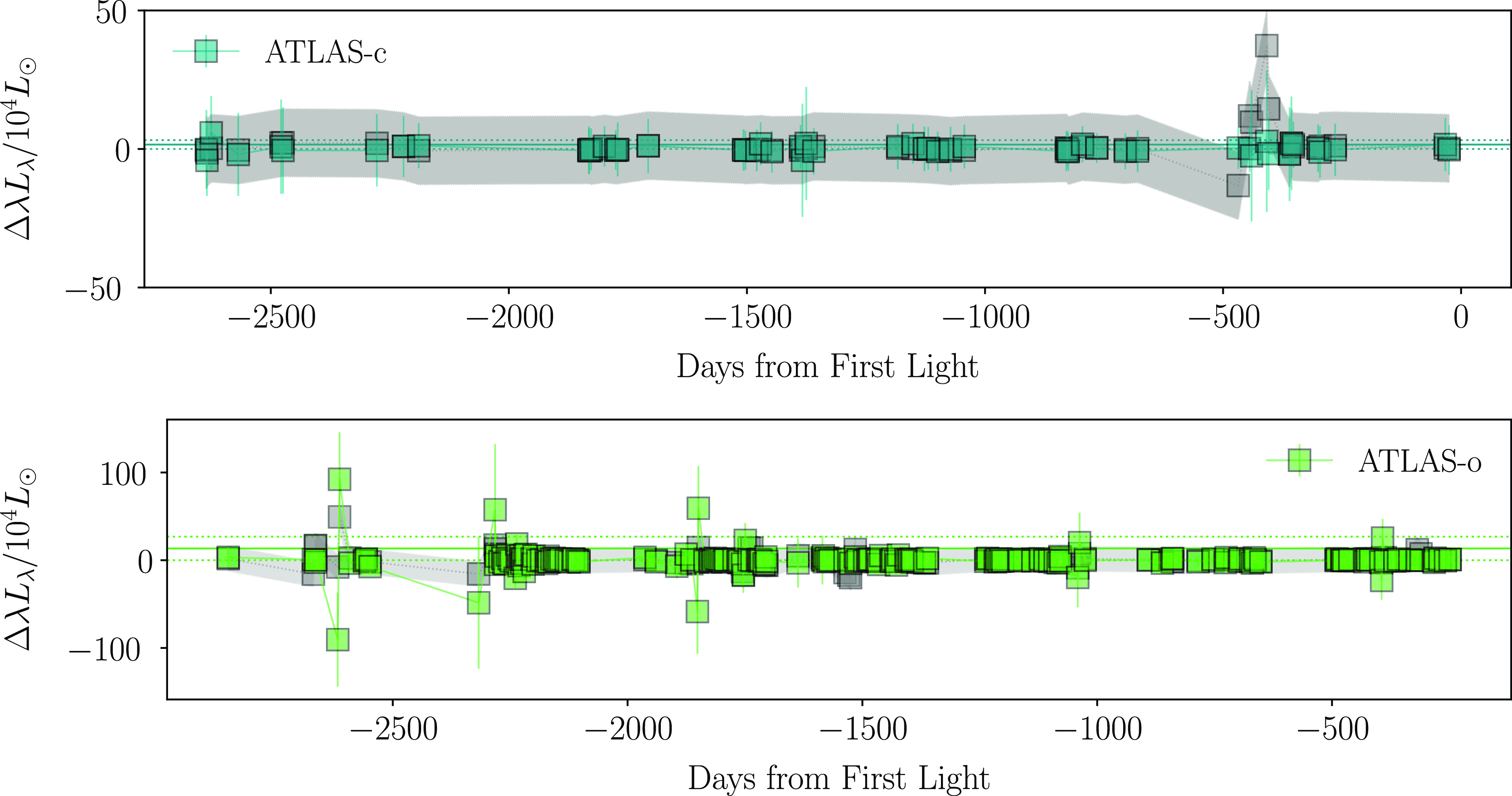
Figure 9. The peak-to-peak luminosity changes of the pre-SN differential luminosity (
 $\Delta\lambda L_{\lambda}$
) of the SN2023ixf progenitor as observed in the ATLAS filters. See Fig. 7 for more details.
$\Delta\lambda L_{\lambda}$
) of the SN2023ixf progenitor as observed in the ATLAS filters. See Fig. 7 for more details.
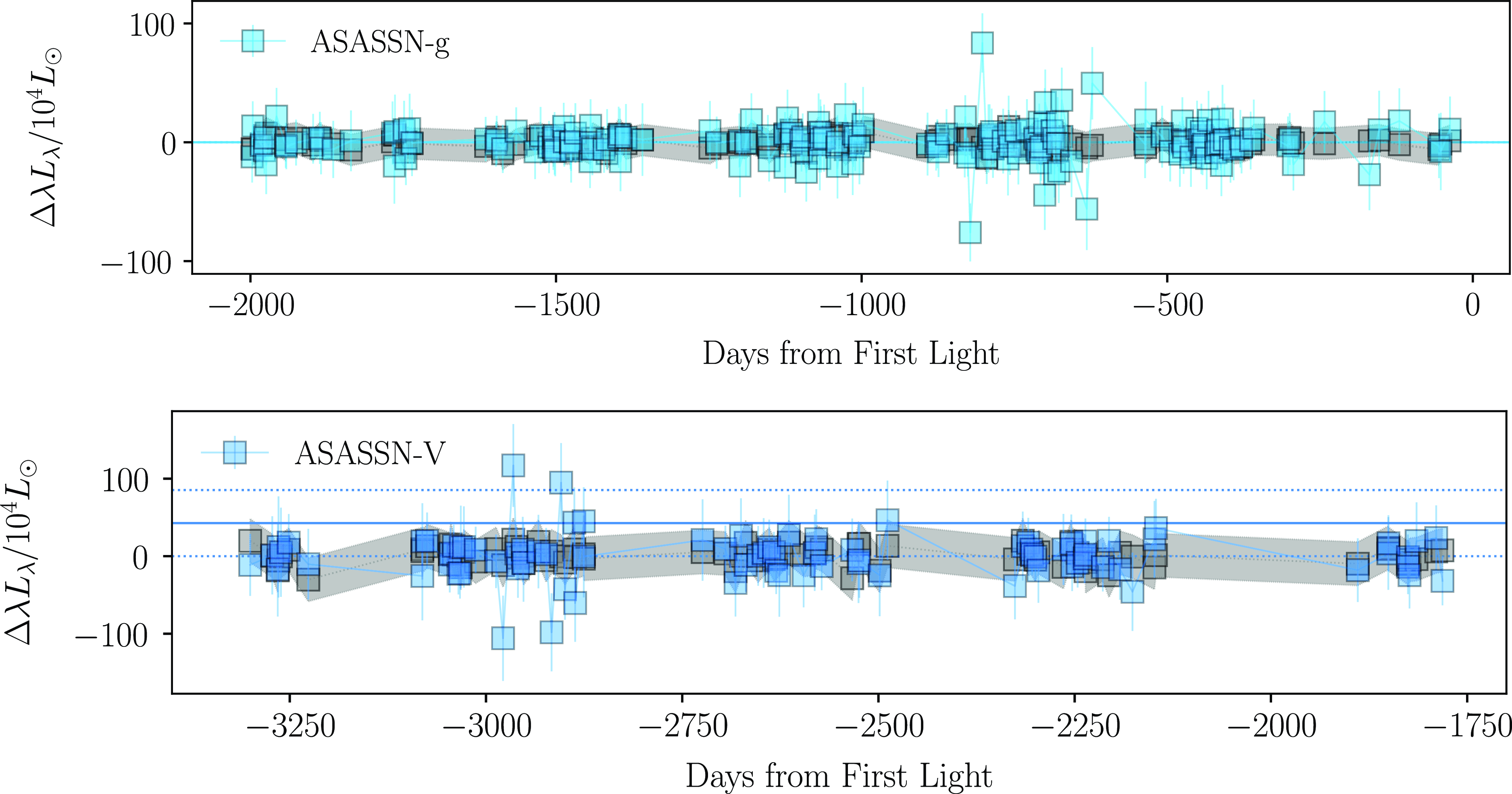
Figure 10. Differential luminosity of the SN2023ixf progenitor as observed in the ASAS-SN filters. See Fig. 7 for more details.
Our plots suggest that for the majority of wavelengths we analysed, the observed scatter in the luminosity at the location of SN2023ixf is consistent with the comparison sample. This suggests that there is no evidence of pre-SN variability in these bands, consistent with the results of Neustadt et al. (Reference Neustadt, Kochanek and Smith2023) and Dong et al. (Reference Dong2023). We do see some evidence of possible dimming detected in the Swift W2 band nearly 6 000 days prior to explosion. However, when one considers the uncertainties in our analysis, these data points lie no more than 1.5
 $\sigma$
from the mean of our controls, suggesting that it may not be significant. Similarly, for the ATLAS o-band, ASAS-SN g-band, and ASAS-SN V-band, the few data points detected above the mean RMS and standard deviation of the controls and RMS of the data have large uncertainties and are thus consistent with the background. This suggests that there is no evidence of stochastic variability in these bands. Using the mean RMS of the ground-based optical light curves (see Table A1), we adopt an upper limit on the variability in these bands of
$\sigma$
from the mean of our controls, suggesting that it may not be significant. Similarly, for the ATLAS o-band, ASAS-SN g-band, and ASAS-SN V-band, the few data points detected above the mean RMS and standard deviation of the controls and RMS of the data have large uncertainties and are thus consistent with the background. This suggests that there is no evidence of stochastic variability in these bands. Using the mean RMS of the ground-based optical light curves (see Table A1), we adopt an upper limit on the variability in these bands of
 $\lesssim$
 $1.0\times10^{5}\, \textrm{L}_{\odot}$
.
$1.0\times10^{5}\, \textrm{L}_{\odot}$
.
To further investigate any long-term trends in the luminosity and search for coherent variability, we also fit the changes in the band luminosities with a simple linear function
 $L(t)=At+B$
. For completeness, we also perform the same fit to the comparison sample. We find that slopes are both positive and negative across the bands and have a mean slope of
$L(t)=At+B$
. For completeness, we also perform the same fit to the comparison sample. We find that slopes are both positive and negative across the bands and have a mean slope of
 $\sim$
 $7.5\times10^{2}\, \textrm{L}_{\odot}$
yr
$7.5\times10^{2}\, \textrm{L}_{\odot}$
yr
 $^{-1}$
. All bands have a slope that is consistent with zero and/or comparable to the mean slope of the control samples. This suggests that there is no evidence of a long-term variability during the final years before explosion down to a luminosity of
$^{-1}$
. All bands have a slope that is consistent with zero and/or comparable to the mean slope of the control samples. This suggests that there is no evidence of a long-term variability during the final years before explosion down to a luminosity of
 $\lesssim$
 $7.5\,\times10^{2}\, \textrm{L}_{\odot}\,$
yr
$7.5\,\times10^{2}\, \textrm{L}_{\odot}\,$
yr
 $^{-1}$
in these bands. This is consistent with that found by Neustadt et al. (Reference Neustadt, Kochanek and Smith2023), Hiramatsu et al. (Reference Hiramatsu2023a) and Dong et al. (Reference Dong2023).
$^{-1}$
in these bands. This is consistent with that found by Neustadt et al. (Reference Neustadt, Kochanek and Smith2023), Hiramatsu et al. (Reference Hiramatsu2023a) and Dong et al. (Reference Dong2023).
4.3 X-ray properties
Due to the proximity of M101, Chandra, XMM-Newton, and Swift have all observed SN2023ixf and the surrounding field in detail. As such, this provides us with the opportunity to place constraints not only on the X-ray emission associated with SN2023ixf as it evolves but also allows us to place constraints on the pre-explosion properties of the progenitor.
In Fig. 11, we show the X-ray light curve from the individual Chandra and XMM-Newton observations, as well as from the combined Swift observations. For the Swift observations, we also show hardness ratios for the emission detected after discovery.
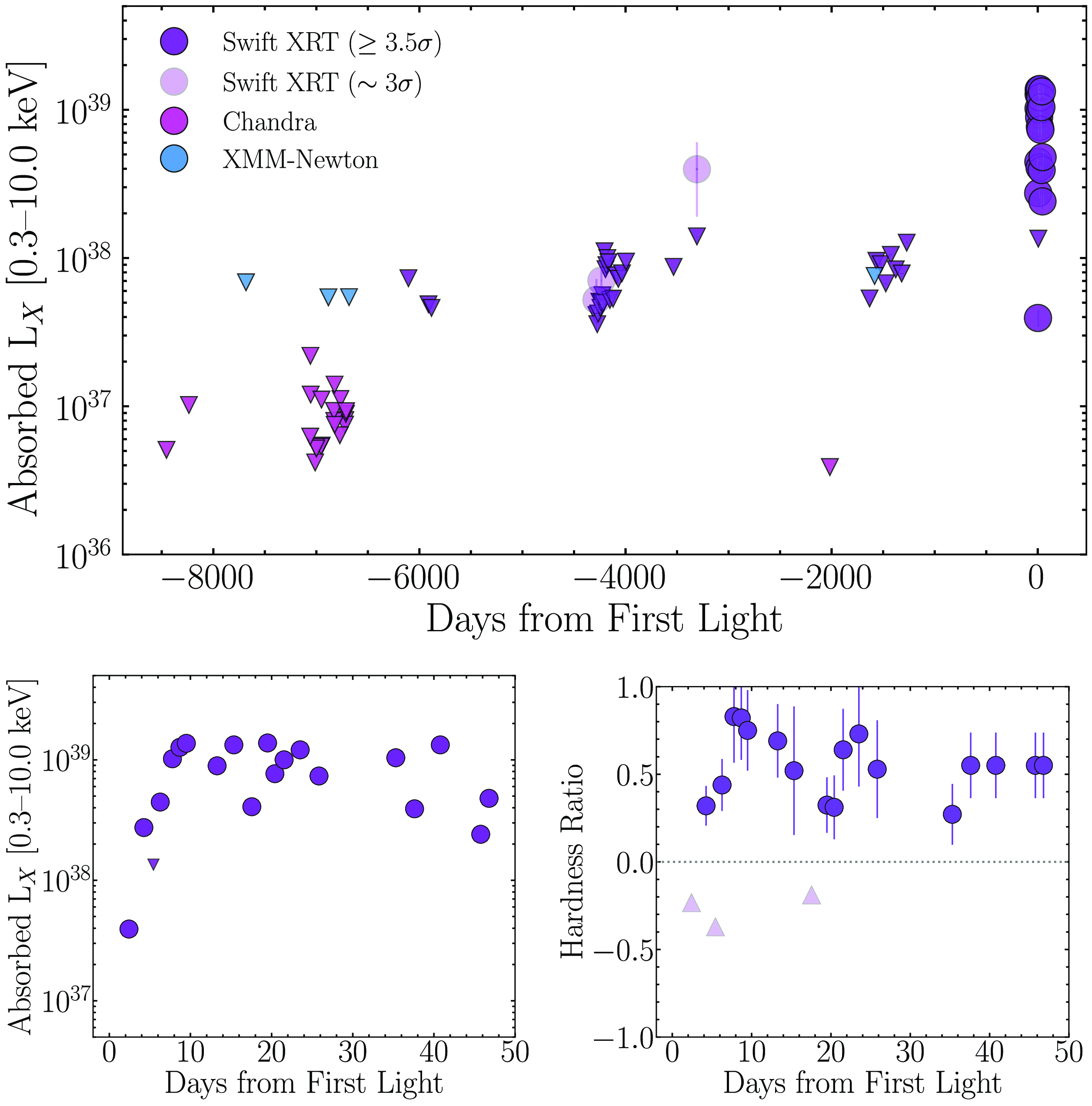
Figure 11.
Upper: Broadband (0.3–10.0 keV) X-ray light curve of SN2023ixf prior to explosion as seen by Chandra, XMM-Newton, and Swift. The down arrows correspond to
 $3\sigma$
(or
$3\sigma$
(or
 $3.5\sigma$
) upper limits and the lightly shaded data points correspond to
$3.5\sigma$
) upper limits and the lightly shaded data points correspond to
 $3\sigma$
X-ray detections which we argue are most likely associated with a nearby HMXB. Lower left: The broadband X-ray light curve of SN2023ixf post-explosion emission as seen by Swift. Note that the error bars are smaller than the plotter markers. Lower right: The hardness ratios of the post-explosion X-ray emission, with up arrows indicating the 3
$3\sigma$
X-ray detections which we argue are most likely associated with a nearby HMXB. Lower left: The broadband X-ray light curve of SN2023ixf post-explosion emission as seen by Swift. Note that the error bars are smaller than the plotter markers. Lower right: The hardness ratios of the post-explosion X-ray emission, with up arrows indicating the 3
 $\sigma$
lower limits. Here, the hardness ratio is derived using
$\sigma$
lower limits. Here, the hardness ratio is derived using
 $\textrm{HR} = (Soft\ Counts - Hard\ Counts)/(\textrm{Soft\ Counts + Hard\ Counts})$
), where Soft Counts corresponds to the count rate in the 0.3–2.0 keV energy band and Hard Counts corresponds to the count rate in the 2.0–10.0 keV energy band. The emission is relatively hard, consistent with a high-temperature thermal component.
$\textrm{HR} = (Soft\ Counts - Hard\ Counts)/(\textrm{Soft\ Counts + Hard\ Counts})$
), where Soft Counts corresponds to the count rate in the 0.3–2.0 keV energy band and Hard Counts corresponds to the count rate in the 2.0–10.0 keV energy band. The emission is relatively hard, consistent with a high-temperature thermal component.
In Fig. 12, we show our Swift X-ray spectrum. To estimate the X-ray luminosity, we convert our extracted count rate from both Swift, Chandra, and XMM-Newton into a flux using WebPIMMSFootnote
f
and we assume an absorbed bremsstrahlung model redshifted to M101 that has a temperature of
 $\Gamma=35$
keV and a column density of
$\Gamma=35$
keV and a column density of
 $N_{H}\sim 3.9\times10^{22}$
cm
$N_{H}\sim 3.9\times10^{22}$
cm
 $^{-2}$
(see Section 4.3.2 for more discussion about the spectral properties).
$^{-2}$
(see Section 4.3.2 for more discussion about the spectral properties).
4.3.1 Pre-explosion
We find no significant evidence of X-ray emission arising from the location of SN2023ixf up to 8 500 days prior to discovery (see Fig. 11 upper panel). The most constraining limit comes from the available Chandra X-ray observations, which are nearly an order of magnitude deeper than the XMM-Newton and Swift limits presented in Fig. 11. As such, to place the deepest constraint on the X-ray emission at the location of SN2023ixf, we merge all Chandra data together and determine a 3
 $\sigma$
count rate upper limit of
$\sigma$
count rate upper limit of
 $8\times10^{-5}$
counts/sec in the 0.3–10.0 keV energy range. All upperlimits are derived following the methodology outlined in Section 2.2 of Auchettl et al. (Reference Auchettl, Guillochon and Ramirez-Ruiz2017). Assuming our best-fit, absorbed-bremsstrahlung model (see Section 4.3.2), this gives us an absorbed flux (0.3–10.0 keV) of
$8\times10^{-5}$
counts/sec in the 0.3–10.0 keV energy range. All upperlimits are derived following the methodology outlined in Section 2.2 of Auchettl et al. (Reference Auchettl, Guillochon and Ramirez-Ruiz2017). Assuming our best-fit, absorbed-bremsstrahlung model (see Section 4.3.2), this gives us an absorbed flux (0.3–10.0 keV) of
 $2.1\times10^{-15}$
erg cm
$2.1\times10^{-15}$
erg cm
 $^{-2}$
s
$^{-2}$
s
 $^{-1}$
, which corresponds to an absorbed (unabsorbed) X-ray luminosity (0.3–10.0 keV) of
$^{-1}$
, which corresponds to an absorbed (unabsorbed) X-ray luminosity (0.3–10.0 keV) of
 $3.3\times10^{36}$
erg s
$3.3\times10^{36}$
erg s
 $^{-1}$
(
$^{-1}$
(
 $5.7\times10^{36}$
erg s
$5.7\times10^{36}$
erg s
 $^{-1}$
). If we use the more recent, but shallower Swift observations that cover up to
$^{-1}$
). If we use the more recent, but shallower Swift observations that cover up to
 $6\,000$
days prior to explosion, we obtain a 3
$6\,000$
days prior to explosion, we obtain a 3
 $\sigma$
count rate upper limit of
$\sigma$
count rate upper limit of
 $2\times10^{-4}$
counts/s in the 0.3–10.0 keV energy range, which corresponds to an unabsorbed X-ray luminosity (0.3–10.0 keV) of
$2\times10^{-4}$
counts/s in the 0.3–10.0 keV energy range, which corresponds to an unabsorbed X-ray luminosity (0.3–10.0 keV) of
 $5.8\times10^{37}$
erg s
$5.8\times10^{37}$
erg s
 $^{-1}$
assuming our best-fit, absorbed-bremsstrahlung model.
$^{-1}$
assuming our best-fit, absorbed-bremsstrahlung model.
Figure 12.
Swift XRT X-ray spectrum obtained by merging all observations taken within the first
 $\sim$
46 days of first light (black data points). Shown as the magenta dot-dashed line is the best-fit, two-component, absorbed bremsstrahlung model. The teal dashed line is our best-fit, single-component, absorbed bremsstrahlung model, while the solid blue line is our best-fit, single-component, absorbed power law model. We have also plotted as an orange dotted line the best-fit model from Grefenstette et al. (Reference Grefenstette, Brightman, Earnshaw, Harrison and Margutti2023) using their second epoch NuSTAR observations. Shown in the bottom panel are the residuals of our best-fit models.
$\sim$
46 days of first light (black data points). Shown as the magenta dot-dashed line is the best-fit, two-component, absorbed bremsstrahlung model. The teal dashed line is our best-fit, single-component, absorbed bremsstrahlung model, while the solid blue line is our best-fit, single-component, absorbed power law model. We have also plotted as an orange dotted line the best-fit model from Grefenstette et al. (Reference Grefenstette, Brightman, Earnshaw, Harrison and Margutti2023) using their second epoch NuSTAR observations. Shown in the bottom panel are the residuals of our best-fit models.
In the left panel of Fig. 4, we show the pre-explosion image from our merged Chandra observations, while in the centre panel of Fig. 4, we have the pre-explosion image created by merging all available pre-explosion Swift data.
We do note that after we merged all Swift observations taken prior to discovery (Fig. 4 middle panel), our analysis suggests the presence of possible weak (
 $\sim$
 $3\sigma$
) X-ray emission coincident with the location of the SN. This is apparent for the observations found between 3 200 and 4 300 days prior to discovery (see Fig. 11 upper panel). Using the same model as above, this emission has an absorbed X-ray luminosity (0.3–10 keV) between
$3\sigma$
) X-ray emission coincident with the location of the SN. This is apparent for the observations found between 3 200 and 4 300 days prior to discovery (see Fig. 11 upper panel). Using the same model as above, this emission has an absorbed X-ray luminosity (0.3–10 keV) between
 $4.8\times10^{37}$
 $\textrm{erg}\,\textrm{s}^{-1}$
and
$\textrm{erg}\,\textrm{s}^{-1}$
and
 $3.7\times10^{38}$
 $\textrm{erg}\,\textrm{s}^{-1}$
. However, we note that close to the location of SN2023ixf, our merged Chandra observations (Fig. 4 left panel) show the HMXBs CXO J140341.1+541903, CXO J140336.1+541924, and [CHP2004] J140339.3+541827 (black, cyan, and magenta crosses in Fig. 4, Evans et al. 2010; Mineo, Gilfanov, & Sunyaev 2012). Unfortunately, due to the spatial resolution of the Swift XRT, it is difficult to disentangle the emission from SN2023ixf and that associated with these nearby binary systems (see Fig. 4 middle panel). As such, we believe it likely that this emission is associated with these sources rather than pre-explosion X-ray emission from the SN itself.
$\textrm{erg}\,\textrm{s}^{-1}$
. However, we note that close to the location of SN2023ixf, our merged Chandra observations (Fig. 4 left panel) show the HMXBs CXO J140341.1+541903, CXO J140336.1+541924, and [CHP2004] J140339.3+541827 (black, cyan, and magenta crosses in Fig. 4, Evans et al. 2010; Mineo, Gilfanov, & Sunyaev 2012). Unfortunately, due to the spatial resolution of the Swift XRT, it is difficult to disentangle the emission from SN2023ixf and that associated with these nearby binary systems (see Fig. 4 middle panel). As such, we believe it likely that this emission is associated with these sources rather than pre-explosion X-ray emission from the SN itself.
4.3.2 Post-explosion
Swift began monitoring the evolution of SN2023ixf
 $\sim$
0.67 days after discovery (MJD = 60083.73), or
$\sim$
0.67 days after discovery (MJD = 60083.73), or
 $\sim$
1.57 days after first light (MJD = 60082.833). Swift did not detect soft X-ray (0.3–10.0 keV) emission until 4.25 days after first light (or 3.36 days after discovery). This is in contrast to the discovery of hard X-rays (
$\sim$
1.57 days after first light (MJD = 60082.833). Swift did not detect soft X-ray (0.3–10.0 keV) emission until 4.25 days after first light (or 3.36 days after discovery). This is in contrast to the discovery of hard X-rays (
 $>3$
keV) at
$>3$
keV) at
 $\sim$
 $3.9$
days after first light using NuSTAR (Grefenstette et al. Reference Grefenstette, Brightman, Earnshaw, Harrison and Margutti2023). However, this is likely not surprising since the significantly enhanced column density measured by Grefenstette et al. (Reference Grefenstette, Brightman, Earnshaw, Harrison and Margutti2023) at this time implies the soft X-rays would be absorbed. To place the strongest constraints on the emission during the first
$3.9$
days after first light using NuSTAR (Grefenstette et al. Reference Grefenstette, Brightman, Earnshaw, Harrison and Margutti2023). However, this is likely not surprising since the significantly enhanced column density measured by Grefenstette et al. (Reference Grefenstette, Brightman, Earnshaw, Harrison and Margutti2023) at this time implies the soft X-rays would be absorbed. To place the strongest constraints on the emission during the first
 $\sim$
4 days after first light, we merged the first 13 post-discovery Swift observations of SN2023ixf and from this calculated a 3
$\sim$
4 days after first light, we merged the first 13 post-discovery Swift observations of SN2023ixf and from this calculated a 3
 $\sigma$
upper limit to the count rate of
$\sigma$
upper limit to the count rate of
 $5\times10^{-4}$
counts/s in the 0.3–10.0 keV energy range.
$5\times10^{-4}$
counts/s in the 0.3–10.0 keV energy range.
At 4.25 days after first light, Swift detected X-ray emission with a significance of
 $>$
$>$
 $4.5\sigma$
(see Fig. 4 lower left panel). This emission has continued to rise nearly an order of magnitude to its current peak count rate of
$4.5\sigma$
(see Fig. 4 lower left panel). This emission has continued to rise nearly an order of magnitude to its current peak count rate of
 $0.0094\pm0.002$
counts/s, corresponding to an absorbed X-ray (0.3–10 keV) luminosity of
$0.0094\pm0.002$
counts/s, corresponding to an absorbed X-ray (0.3–10 keV) luminosity of
 $(1.6\pm0.4)\times10^{39}$
erg s
$(1.6\pm0.4)\times10^{39}$
erg s
 $^{-1}$
assuming our best-fit bremsstrahlung model discussed below.
$^{-1}$
assuming our best-fit bremsstrahlung model discussed below.
Unfortunately, due to the relatively short exposures of the Swift observations, we are unable to extract a spectrum from each individual observation. As such, we merged all available post-explosion Swift observations and extracted a spectrum to constrain the nature of this emission. This spectrum describes the soft X-ray emission arising from SN2023ixf in the first
 $\sim$
46 days since first light and its best-fit spectral model discussed below is shown in Fig. 12.
$\sim$
46 days since first light and its best-fit spectral model discussed below is shown in Fig. 12.
To study the nature of this emission, we fit the 0.3–10.0 keV spectrum using an absorbed power law redshifted to the host galaxy (XSPEC model: tbabs*zashift*powerlaw), similar to that done by Grefenstette et al. (Reference Grefenstette, Brightman, Earnshaw, Harrison and Margutti2023). However, due to the emission seen at energies
 $\lesssim$
2 keV, we find that our best-fit model with a column density of
$\lesssim$
2 keV, we find that our best-fit model with a column density of
 $N_{H}=(3.4_{-1.1}^{+1.5}\times10^{22}$
) cm
$N_{H}=(3.4_{-1.1}^{+1.5}\times10^{22}$
) cm
 $^{-2}$
and a photon index of
$^{-2}$
and a photon index of
 $\Gamma=1.6\pm0.5$
fails to fit the emission seen at these lower energies. However, if we instead fit the spectrum at energies
$\Gamma=1.6\pm0.5$
fails to fit the emission seen at these lower energies. However, if we instead fit the spectrum at energies
 $\gtrsim$
2 keV, our fit is consistent with that of Grefenstette (Reference Grefenstette2023) using NuSTAR data.
$\gtrsim$
2 keV, our fit is consistent with that of Grefenstette (Reference Grefenstette2023) using NuSTAR data.
Assuming that this power law results from either X-ray synchrotron emission or inverse Compton (IC) scattering as is typical for X-ray emitting SNe (e.g. Chevalier & Fransson Reference Chevalier and Fransson2006), then the observed X-ray flux would be proportional to
 $\nu^{1-\Gamma}$
, where
$\nu^{1-\Gamma}$
, where
 $\nu$
is the frequency and
$\nu$
is the frequency and
 $\Gamma$
is the photon index derived from our best-fit power law. As such, a value of
$\Gamma$
is the photon index derived from our best-fit power law. As such, a value of
 $\Gamma=1.6$
as derived above, would indicate a hard X-ray spectrum, which is consistent with that seen from other X-ray bright SNe (e.g. Chandra Reference Chandra2018).
$\Gamma=1.6$
as derived above, would indicate a hard X-ray spectrum, which is consistent with that seen from other X-ray bright SNe (e.g. Chandra Reference Chandra2018).
However, for SNe that are interacting with a dense CSM, their fast shocks result in hard X-ray emission that is dominated by thermal bremsstrahlung emission with temperatures
 $>$
1 keV (e.g. as seen in SN2014C, SN2010jl, and SN2006jd: Chandra et al. Reference Chandra2012, Reference Chandra, Chevalier, Chugai, Fransson and Soderberg2015; Katsuda et al. Reference Katsuda2016; Margutti et al. Reference Margutti2017; Thomas et al. Reference Thomas2022; Brethauer et al. Reference Brethauer2022). Since these high-temperature thermal models can mimic hard power laws, we also fit the spectrum using an absorbed, thermal-bremsstrahlung model (XSPEC model: tbabs*zashift*bremss). As with our best-fit power law model, our best-fit thermal model with a column density of
$>$
1 keV (e.g. as seen in SN2014C, SN2010jl, and SN2006jd: Chandra et al. Reference Chandra2012, Reference Chandra, Chevalier, Chugai, Fransson and Soderberg2015; Katsuda et al. Reference Katsuda2016; Margutti et al. Reference Margutti2017; Thomas et al. Reference Thomas2022; Brethauer et al. Reference Brethauer2022). Since these high-temperature thermal models can mimic hard power laws, we also fit the spectrum using an absorbed, thermal-bremsstrahlung model (XSPEC model: tbabs*zashift*bremss). As with our best-fit power law model, our best-fit thermal model with a column density of
 $N_{H}=(2.4_{-0.5}^{+0.7}\times10^{22}$
) cm
$N_{H}=(2.4_{-0.5}^{+0.7}\times10^{22}$
) cm
 $^{-2}$
and a temperature of
$^{-2}$
and a temperature of
 $kT=33_{-30}^{+50}$
keV fails to fit the emission seen at lower energies (see Fig. 12). Nonetheless, the thermal model is a better fit than the single power law and is consistent with that found by Chandra et al. (Reference Chandra, Maeda, Chevalier, Nayana and Ray2023b) using Chandra and by Grefenstette et al. (Reference Grefenstette, Brightman, Earnshaw, Harrison and Margutti2023) using a second epoch of NuSTAR observations taken
$kT=33_{-30}^{+50}$
keV fails to fit the emission seen at lower energies (see Fig. 12). Nonetheless, the thermal model is a better fit than the single power law and is consistent with that found by Chandra et al. (Reference Chandra, Maeda, Chevalier, Nayana and Ray2023b) using Chandra and by Grefenstette et al. (Reference Grefenstette, Brightman, Earnshaw, Harrison and Margutti2023) using a second epoch of NuSTAR observations taken
 $\sim$
10 days after first light.
$\sim$
10 days after first light.
In an attempt to explain this excess seen at lower energies, we tried adding either an absorbed bremsstrahlung model or an absorbed power law model to our best-fit bremsstrahlung model. This is similar to what was done for SN2010jl (Fransson et al. Reference Fransson2014; Chandra et al. Reference Chandra, Chevalier, Chugai, Fransson and Soderberg2015), whose Chandra and Swift observations showed the presence of an additional soft component
 $\sim$
40–600 days after discovery, which the authors attributed to the cooling of the shock front. We find that an additional bremsstrahlung model significantly improves the fit. With this additional component, the spectrum is best fit (reduced
$\sim$
40–600 days after discovery, which the authors attributed to the cooling of the shock front. We find that an additional bremsstrahlung model significantly improves the fit. With this additional component, the spectrum is best fit (reduced
 $\chi^{2}$
= 1.02) with a column density of
$\chi^{2}$
= 1.02) with a column density of
 $N_{H,soft}=(0.9_{-0.3}^{+0.5}\times10^{22}$
) cm
$N_{H,soft}=(0.9_{-0.3}^{+0.5}\times10^{22}$
) cm
 $^{-2}$
and a temperature of
$^{-2}$
and a temperature of
 $kT_{soft}=0.3\pm0.1$
keV for the low-energy (soft) component, and a column density of
$kT_{soft}=0.3\pm0.1$
keV for the low-energy (soft) component, and a column density of
 $N_{H,hard}=(3.9_{-1.7}^{+1.2}\times10^{22}$
) cm
$N_{H,hard}=(3.9_{-1.7}^{+1.2}\times10^{22}$
) cm
 $^{-2}$
and a temperature of
$^{-2}$
and a temperature of
 $kT_{hard}=35_{-27}^{+110}$
keV for the high-energy (hard) component. This fit and its residuals are plotted in magenta in Fig. 12.
$kT_{hard}=35_{-27}^{+110}$
keV for the high-energy (hard) component. This fit and its residuals are plotted in magenta in Fig. 12.
To verify whether this additional soft X-ray component can be attributed to SN2023ixf or instead arises from the nearby soft X-ray sources shown in Fig. 4, we extracted a merged Swift spectrum from the location of SN2023ixf prior to explosion. From this analysis, we find that the additional bremsstrahlung component required to accurately model the emission from SN2023ixf at energies less than 2 keV indeed arises from the supernova itself and does not arise from the complex X-ray environment in which SN2023ixf is situated.
To derive the fluxes and luminosities required for our analysis in Section 5, we use our best-fit column density (
 $N_{H,hard}=3.9\times10^{22}$
cm
$N_{H,hard}=3.9\times10^{22}$
cm
 $^{-2}$
) and temperature (
$^{-2}$
) and temperature (
 $kT_{hard}=35$
keV) associated with the high-temperature component of our best-fit, two-component, bremsstrahlung model. This high temperature is thought to result from the expanding forward shock, meaning we can use this temperature to place constraints on the shock velocity and compare our results to those determined from optical spectra. To calculate the shock velocity, we use
$kT_{hard}=35$
keV) associated with the high-temperature component of our best-fit, two-component, bremsstrahlung model. This high temperature is thought to result from the expanding forward shock, meaning we can use this temperature to place constraints on the shock velocity and compare our results to those determined from optical spectra. To calculate the shock velocity, we use
 $\nu_{s} = [(16 k_{B}T_{sh})/(3\mu m_{H})]^{1/2}$
, where
$\nu_{s} = [(16 k_{B}T_{sh})/(3\mu m_{H})]^{1/2}$
, where
 $\nu_{s}$
is the shock velocity,
$\nu_{s}$
is the shock velocity,
 $k_{B}T_{sh}$
is our shock temperature,
$k_{B}T_{sh}$
is our shock temperature,
 $\mu=0.604$
is the mean atomic weight,
$\mu=0.604$
is the mean atomic weight,
 $k_{B}$
is Boltzmann’s constant, and
$k_{B}$
is Boltzmann’s constant, and
 $m_{H}$
is the mass of hydrogen (e.g. Auchettl, Slane, & Castro Reference Auchettl, Slane and Castro2014). Using this equation and our temperature from the high-energy component of our best-fit, two-component bremsstrahlung model, we find a shock velocity of
$m_{H}$
is the mass of hydrogen (e.g. Auchettl, Slane, & Castro Reference Auchettl, Slane and Castro2014). Using this equation and our temperature from the high-energy component of our best-fit, two-component bremsstrahlung model, we find a shock velocity of
 $5\,440_{-2840}^{+5630}$
 $\textrm{km} \,\textrm{ s}^{-1}$
which is consistent with that found by Jacobson-Galan et al. (Reference Jacobson-Galan2023) using H
$\textrm{km} \,\textrm{ s}^{-1}$
which is consistent with that found by Jacobson-Galan et al. (Reference Jacobson-Galan2023) using H
 $\alpha$
absorption profiles and Grefenstette et al. (Reference Grefenstette, Brightman, Earnshaw, Harrison and Margutti2023) using NuSTAR data.
$\alpha$
absorption profiles and Grefenstette et al. (Reference Grefenstette, Brightman, Earnshaw, Harrison and Margutti2023) using NuSTAR data.
5. Discussion
5.1 Lack of precursor variability from optical to X-rays
One way of constraining pre-explosion mass loss is to search for variable precursor emission from the progenitor. Evidence of end-of-life mass loss may also be seen in the form of precursor outbursts that are detected in the weeks to months before the main SN explosion (Ofek et al. Reference Ofek2014). These outbursts are thought to be associated with the different stages of nuclear burning (e.g. Fuller Reference Fuller2017; Shiode & Quataert Reference Shiode and Quataert2014; Wu & Fuller Reference Wu and Fuller2021), instabilities in nuclear shell burning (e.g. Woosley et al. Reference Woosley, Heger and Weaver2002), or interaction with a binary companion (e.g. Matsuoka & Sawada Reference Matsuoka and Sawada2023).
Such an analysis has been performed for SN2023ixf in both the mid- and near-IR using Spitzer and ground-based observations, respectively (Kilpatrick et al. Reference Kilpatrick2023; Jencson et al. Reference Jencson2023; Soraisam et al. Reference Soraisam2023b), in some optical bands (Neustadt et al. Reference Neustadt, Kochanek and Smith2023; Dong et al. Reference Dong2023), and in the UV with GALEX (Flinner et al. Reference Flinner, Tucker, Beacom and Shappee2023). Kilpatrick et al. (Reference Kilpatrick2023), Jencson et al. (Reference Jencson2023), and Soraisam et al. (Reference Soraisam2023b) showed that the progenitor exhibited significant variability with a period of
 $\sim$
1 000–1 200 days and an amplitude similar to the more luminous population of pulsating, dusty RSGs. However, Jencson et al. (Reference Jencson2023) found no evidence for re-brightening due to eruptive, pre-SN outbursts predicted from early, post-SN observations (e.g. Jacobson-Galan et al. Reference Jacobson-Galan2023), nor due to those expected from instabilities on the timescales of the final nuclear burning stages (e.g. Woosley et al. Reference Woosley, Heger and Weaver2002). Similarly, Neustadt et al. (Reference Neustadt, Kochanek and Smith2023), Hiramatsu et al. (Reference Hiramatsu2023a) and Dong et al. (Reference Dong2023) found no evidence of variability in the optical, with Neustadt et al. (Reference Neustadt, Kochanek and Smith2023) deriving a limit of
$\sim$
1 000–1 200 days and an amplitude similar to the more luminous population of pulsating, dusty RSGs. However, Jencson et al. (Reference Jencson2023) found no evidence for re-brightening due to eruptive, pre-SN outbursts predicted from early, post-SN observations (e.g. Jacobson-Galan et al. Reference Jacobson-Galan2023), nor due to those expected from instabilities on the timescales of the final nuclear burning stages (e.g. Woosley et al. Reference Woosley, Heger and Weaver2002). Similarly, Neustadt et al. (Reference Neustadt, Kochanek and Smith2023), Hiramatsu et al. (Reference Hiramatsu2023a) and Dong et al. (Reference Dong2023) found no evidence of variability in the optical, with Neustadt et al. (Reference Neustadt, Kochanek and Smith2023) deriving a limit of
 $<$
100
$<$
100
 $\textrm{L}_{\odot}$
yr
$\textrm{L}_{\odot}$
yr
 $^{-1}$
, suggesting that the progenitor did not undergo a luminous outburst within the 15 yr prior to discovery or it would have led to changes in the optical depth, making it detectable.
$^{-1}$
, suggesting that the progenitor did not undergo a luminous outburst within the 15 yr prior to discovery or it would have led to changes in the optical depth, making it detectable.
We search for evidence of possible pre-explosion variability/emission not only in the bands similar to that observed by Neustadt et al. (Reference Neustadt, Kochanek and Smith2023), Hiramatsu et al. (Reference Hiramatsu2023a) and Dong et al. (Reference Dong2023) but also using X-ray data from Swift, and UV/optical data from the Swift UVOT, as well as that observed using ATLAS, ZTF, and ASAS-SN. Here, we consider not only emission during the last year prior to discovery but also the possibility of pre-explosion variability spanning nearly 2 decades of observations.
Following the analysis presented in Johnson et al. (Reference Johnson, Kochanek and Adams2017, Reference Johnson, Kochanek and Adams2018) and Neustadt et al. (Reference Neustadt, Kochanek and Smith2023) (see Section 4.2), we found no evidence of variability in optical to UV bands as detected by Swift, ASAS-SN, ZTF, and ATLAS in the
 $\sim$
20 yr prior to explosion. This is consistent with that found by Neustadt et al. (Reference Neustadt, Kochanek and Smith2023), Hiramatsu et al. (Reference Hiramatsu2023a) and Dong et al. (Reference Dong2023). We derived a limit on the stochastic variability of
$\sim$
20 yr prior to explosion. This is consistent with that found by Neustadt et al. (Reference Neustadt, Kochanek and Smith2023), Hiramatsu et al. (Reference Hiramatsu2023a) and Dong et al. (Reference Dong2023). We derived a limit on the stochastic variability of
 $\lesssim$
 $1\times10^{5}\, \textrm{L}_{\odot}$
and on the long-term variability of
$1\times10^{5}\, \textrm{L}_{\odot}$
and on the long-term variability of
 $<$
$<$
 $7.5\times10^{2}\, \textrm{L}_{\odot}$
yr
$7.5\times10^{2}\, \textrm{L}_{\odot}$
yr
 $^{-1}$
. These values are consistent with that obtained by Neustadt et al. (Reference Neustadt, Kochanek and Smith2023). In X-rays, we find no evidence of pre-explosion emission down to a limit of
$^{-1}$
. These values are consistent with that obtained by Neustadt et al. (Reference Neustadt, Kochanek and Smith2023). In X-rays, we find no evidence of pre-explosion emission down to a limit of
 $5.8\times10^{37}$
erg s
$5.8\times10^{37}$
erg s
 $^{-1}$
in the 16 yr (
$^{-1}$
in the 16 yr (
 $\sim$
 $6\,000$
days) prior to explosion.
$6\,000$
days) prior to explosion.
Neustadt et al. (Reference Neustadt, Kochanek and Smith2023) suggested that due to the heavy obscuration associated with the source, any short-lived outburst with a peak luminosity
 $\gtrsim$
 $5\times10^{5}\, \textrm{L}_{\odot}$
should lead to a detectable signature in the decade-long light curves, unless it lined up with a seasonal gap. Due to the extensive coverage by Swift, ASAS-SN, ATLAS, and ZTF prior to explosion, our results suggest that there was no bright, short-lived, pre-SN outburst within the
$5\times10^{5}\, \textrm{L}_{\odot}$
should lead to a detectable signature in the decade-long light curves, unless it lined up with a seasonal gap. Due to the extensive coverage by Swift, ASAS-SN, ATLAS, and ZTF prior to explosion, our results suggest that there was no bright, short-lived, pre-SN outburst within the
 $\sim$
5 yr prior to explosion, similar to that found by Dong et al. (Reference Dong2023) and Hiramatsu et al. (Reference Hiramatsu2023a). In addition, our results for Swift, ASAS-SN, ATLAS, and ZTF in Table A1 require that any outburst had a luminosity
$\sim$
5 yr prior to explosion, similar to that found by Dong et al. (Reference Dong2023) and Hiramatsu et al. (Reference Hiramatsu2023a). In addition, our results for Swift, ASAS-SN, ATLAS, and ZTF in Table A1 require that any outburst had a luminosity
 $\lesssim$
 $1\times10^{5}\, \textrm{L}_{\odot}$
. This is consistent with the suggestion by Neustadt et al. (Reference Neustadt, Kochanek and Smith2023), Dong et al. (Reference Dong2023), and Jencson et al. (Reference Jencson2023) that there was no luminous, short-lived outburst within the 15 yr prior to explosion. In addition, the lack of variability detected by Hiramatsu et al. (Reference Hiramatsu2023a) is consistent with their dense, confined CSM models that take into account pre-existing dust surrounding the progenitor. However, these findings are in contrast to the prediction by Jacobson-Galan et al. (Reference Jacobson-Galan2023) that the dense CSM inferred from early spectra could have arisen if the progenitor experienced periods of enhanced mass loss during the final 3–6 yr before core collapse.
$1\times10^{5}\, \textrm{L}_{\odot}$
. This is consistent with the suggestion by Neustadt et al. (Reference Neustadt, Kochanek and Smith2023), Dong et al. (Reference Dong2023), and Jencson et al. (Reference Jencson2023) that there was no luminous, short-lived outburst within the 15 yr prior to explosion. In addition, the lack of variability detected by Hiramatsu et al. (Reference Hiramatsu2023a) is consistent with their dense, confined CSM models that take into account pre-existing dust surrounding the progenitor. However, these findings are in contrast to the prediction by Jacobson-Galan et al. (Reference Jacobson-Galan2023) that the dense CSM inferred from early spectra could have arisen if the progenitor experienced periods of enhanced mass loss during the final 3–6 yr before core collapse.
The lack of variability seen in these wavelengths may not be so surprising. Currently, there have been nearly 30 SNe that have exhibited pre-SN activity (e.g. Jacobson-Galán et al. Reference Jacobson-Galán2022a; Strotjohann et al. Reference Strotjohann2021), but current surveys searching for precursors and SN progenitors (e.g. Johnson et al. Reference Johnson, Kochanek and Adams2017, Reference Johnson, Kochanek and Adams2018) suggest that not all SNe exhibit luminous precursors and at most,
 $\sim$
2.5% of all core-collapse SNe or
$\sim$
2.5% of all core-collapse SNe or
 $\sim$
25% of Type IIn SNe produce luminous, eruptive outbursts prior to explosion (Strotjohann et al. Reference Strotjohann2021). As such, it is possible that the formation of SN2023ixf’s CSM results not from episodic mass loss, but rather from binary interactions (Matsuoka & Sawada Reference Matsuoka and Sawada2023) that gave rise to its observed asymmetry (Smith et al. Reference Smith2023; Vasylyev et al. Reference Vasylyev2023). Here, the collision of the winds from the two stars in the binary system would produce a high-density (and possibly asymmetric) CSM around the progenitor (e.g. Kochanek Reference Kochanek2019).
$\sim$
25% of Type IIn SNe produce luminous, eruptive outbursts prior to explosion (Strotjohann et al. Reference Strotjohann2021). As such, it is possible that the formation of SN2023ixf’s CSM results not from episodic mass loss, but rather from binary interactions (Matsuoka & Sawada Reference Matsuoka and Sawada2023) that gave rise to its observed asymmetry (Smith et al. Reference Smith2023; Vasylyev et al. Reference Vasylyev2023). Here, the collision of the winds from the two stars in the binary system would produce a high-density (and possibly asymmetric) CSM around the progenitor (e.g. Kochanek Reference Kochanek2019).
5.2 Pre-explosion mass loss
Using pre- and post-explosion X-ray observations, it is possible to place constraints on the density of the CSM. This is because the mass that is ejected from the progenitor star during the pre-SN phase becomes the CSM with which the SN ejecta interacts following the explosion.
5.2.1 Pre-explosion X-ray constraints on the mass loss
The interaction of the shock with the CSM can power the resulting SN and produce both non-thermal X-rays and radio emission (e.g. Margutti et al. Reference Margutti2014, Reference Margutti2017). However, evidence of mass loss may also be seen as precursor outbursts in X-rays and at other wavelengths. Due to its proximity, the location of SN2023ixf has been extensively observed using Chandra, Swift, and XMM-Newton (see Fig. 4). Similar to our analysis of the pre-explosion optical and UV light curves (see Section 4.2), our pre-explosion X-ray analysis also finds no evidence of luminous precursor emission at higher energies.
Using our deep pre-explosion Chandra observation, we can place constraints on the pre-explosion mass loss. Since we find no evidence of outbursts that would be consistent with an eruption scenario, we assume that any precursor emission would have been generated by a wind with a mass-loss rate
 $\dot{M}$
and wind velocity
$\dot{M}$
and wind velocity
 $v_{w}$
. Equation 30 from Matsumoto & Metzger (Reference Matsumoto and Metzger2022) allows us to estimate the mass-loss rate using the progenitor mass (
$v_{w}$
. Equation 30 from Matsumoto & Metzger (Reference Matsumoto and Metzger2022) allows us to estimate the mass-loss rate using the progenitor mass (
 $M_{\star}$
), wind velocity (
$M_{\star}$
), wind velocity (
 $v_{w}$
), and precursor luminosity (
$v_{w}$
), and precursor luminosity (
 $L_{pre}$
) according to:
$L_{pre}$
) according to:
 \begin{equation} \dot{M}\simeq 1.5\left(\frac{M_\star}{10\,\textrm{ M}_{\odot}}\right)^{-2}\!\left (\frac{v_{\textrm{w}}}{10^3{\,\textrm{km}\,\textrm{ s}^{-1}}}\right)^{-2}\!\left(\frac{L_{\textrm{pre}}}{10^{40}{\,\textrm{erg}\,\textrm{s}^{-1}}}\right)^{3} \textrm{M}_{\odot} \, \textrm{yr}^{-1}.\end{equation}
Adopting a progenitor mass between 11 and 20
 $\textrm{M}_{\odot}$
(Kilpatrick et al. Reference Kilpatrick2023; Jencson et al. Reference Jencson2023; Soraisam et al. Reference Soraisam2023b), a wind velocity of 50 km s
$\textrm{M}_{\odot}$
(Kilpatrick et al. Reference Kilpatrick2023; Jencson et al. Reference Jencson2023; Soraisam et al. Reference Soraisam2023b), a wind velocity of 50 km s
 $^{-1}$
, and using for
$^{-1}$
, and using for
 $L_{pre}$
our unabsorbed 3
$L_{pre}$
our unabsorbed 3
 $\sigma$
upper limit to the X-ray emission from Chandra observations that span
$\sigma$
upper limit to the X-ray emission from Chandra observations that span
 $>$
$>$
 $6\,000$
days (
$6\,000$
days (
 $>$
18 yr) prior to explosion (
$>$
18 yr) prior to explosion (
 $L_{X}<5.7\times10^{36}$
erg s
$L_{X}<5.7\times10^{36}$
erg s
 $^{-1}$
), we get
$^{-1}$
), we get
 $\dot{M}=(3-9)\times10^{-8} \textrm{M}_{\odot}$
yr
$\dot{M}=(3-9)\times10^{-8} \textrm{M}_{\odot}$
yr
 $^{-1}$
. If we use the more recent Swift upper limit derived from merging all available Swift pre-explosion observations that cover
$^{-1}$
. If we use the more recent Swift upper limit derived from merging all available Swift pre-explosion observations that cover
 $<$
$<$
 $6\,000$
days (
$6\,000$
days (
 $<$
16 yr) prior to explosion (
$<$
16 yr) prior to explosion (
 $L_{X}<5.8\times10^{37}$
erg s
$L_{X}<5.8\times10^{37}$
erg s
 $^{-1}$
), we get
$^{-1}$
), we get
 $\dot{M}=(3-10)\times10^{-5} \, \textrm{M}_{\odot}$
yr
$\dot{M}=(3-10)\times10^{-5} \, \textrm{M}_{\odot}$
yr
 $^{-1}$
.
$^{-1}$
.
The mass-loss rate derived using the more recent Swift constraint (covering
 $<$
16 yr prior to explosion) is consistent with the mass loss expected for normal RSGs (Beasor et al. Reference Beasor2020) and that derived by Neustadt et al. (Reference Neustadt, Kochanek and Smith2023) and Jencson et al. (Reference Jencson2023), who modelled the IR SED of the progenitor assuming it is surrounded by a dusty CSM. However, it is lower than that derived by Jacobson-Galan et al. (Reference Jacobson-Galan2023) from early spectra and Soraisam et al. (Reference Soraisam2023c) who used the mass-loss prescription of Goldman et al. (Reference Goldman2017) and a SED-independent luminosity for the progenitor. As our mass-loss rate from deep Chandra observations spanning
$<$
16 yr prior to explosion) is consistent with the mass loss expected for normal RSGs (Beasor et al. Reference Beasor2020) and that derived by Neustadt et al. (Reference Neustadt, Kochanek and Smith2023) and Jencson et al. (Reference Jencson2023), who modelled the IR SED of the progenitor assuming it is surrounded by a dusty CSM. However, it is lower than that derived by Jacobson-Galan et al. (Reference Jacobson-Galan2023) from early spectra and Soraisam et al. (Reference Soraisam2023c) who used the mass-loss prescription of Goldman et al. (Reference Goldman2017) and a SED-independent luminosity for the progenitor. As our mass-loss rate from deep Chandra observations spanning
 $>$
18 yr prior to explosion is even more constraining, this could suggest that the mass loss may have increased over the two decades prior to explosion. This is consistent with the results of Jencson et al. (Reference Jencson2023), whose findings suggest that the progenitor had a steady but enhanced wind that developed over the final decade or more prior to explosion.
$>$
18 yr prior to explosion is even more constraining, this could suggest that the mass loss may have increased over the two decades prior to explosion. This is consistent with the results of Jencson et al. (Reference Jencson2023), whose findings suggest that the progenitor had a steady but enhanced wind that developed over the final decade or more prior to explosion.
5.2.2 Post-explosion X-ray constraints on the mass loss
Post-explosion X-ray observations can also be used to place deep constraints on the properties of the CSM for Type Ia (e.g. Margutti et al. Reference Margutti2012), Type Ibc (e.g. Drout et al. Reference Drout2016), and Type Ib/IIn SNe such as SN2014c (e.g. Margutti et al. Reference Margutti2014). In these papers, they follow the formalism that within the first
 $\sim$
month of evolution, the X-ray emission is dominated by IC scattering that results in photons from the photosphere being upscattered to X-ray energies by relativistic electrons from the expanding SN shock front (Björnsson & Fransson Reference Björnsson and Fransson2004; Chevalier & Fransson Reference Chevalier and Fransson2006; Margutti et al. Reference Margutti2012, Reference Margutti2017).
$\sim$
month of evolution, the X-ray emission is dominated by IC scattering that results in photons from the photosphere being upscattered to X-ray energies by relativistic electrons from the expanding SN shock front (Björnsson & Fransson Reference Björnsson and Fransson2004; Chevalier & Fransson Reference Chevalier and Fransson2006; Margutti et al. Reference Margutti2012, Reference Margutti2017).
If the progenitor lost material at a constant rate
 $\dot{M}$
, which seems to be consistent with the results presented in Section 5.2 and those derived by Jencson et al. (Reference Jencson2023), we can use the formalism presented in Equations A7 and A8 of Margutti et al. (Reference Margutti2012) and Margutti et al. (Reference Margutti2018b) to calculate the wind density (
$\dot{M}$
, which seems to be consistent with the results presented in Section 5.2 and those derived by Jencson et al. (Reference Jencson2023), we can use the formalism presented in Equations A7 and A8 of Margutti et al. (Reference Margutti2012) and Margutti et al. (Reference Margutti2018b) to calculate the wind density (
 $\dot{M}/v_{w}$
). We can also use the fact that Swift observations of SN2023ixf taken within the first
$\dot{M}/v_{w}$
). We can also use the fact that Swift observations of SN2023ixf taken within the first
 $\sim$
 $3.3$
days after first light showed no soft X-rays. Merging these observations, we derive a
$3.3$
days after first light showed no soft X-rays. Merging these observations, we derive a
 $3\sigma$
upper limit to the unabsorbed luminosity in the 0.3–10.0 keV energy band of
$3\sigma$
upper limit to the unabsorbed luminosity in the 0.3–10.0 keV energy band of
 $7.2\times10^{38}$
erg s
$7.2\times10^{38}$
erg s
 $^{-1}$
.
$^{-1}$
.
To calculate the corresponding IC emission, we assume the following: that the ejecta has a density profile that follows
 $\rho \propto R^{-n}$
with
$\rho \propto R^{-n}$
with
 $n\sim9$
as appropriate for compact progenitors (Matzner & McKee Reference Matzner and McKee1999), that the shock-accelerated electrons are best described by a power-law distribution with an index of 3, that 1% of the post-shock energy density goes in relativistic electrons (Reynolds et al. Reference Reynolds, Williams, Borkowski and Long2021), that the shock velocity depends on the wind velocity, explosion energy, ejecta mass, and CSM density which is described by
$n\sim9$
as appropriate for compact progenitors (Matzner & McKee Reference Matzner and McKee1999), that the shock-accelerated electrons are best described by a power-law distribution with an index of 3, that 1% of the post-shock energy density goes in relativistic electrons (Reynolds et al. Reference Reynolds, Williams, Borkowski and Long2021), that the shock velocity depends on the wind velocity, explosion energy, ejecta mass, and CSM density which is described by
 $\rho_{CSM}=\dot{M}/4\pi \nu_{w}R^{2}$
, and that
$\rho_{CSM}=\dot{M}/4\pi \nu_{w}R^{2}$
, and that
 $L_{X-ray}\propto L_{bol}$
, where
$L_{X-ray}\propto L_{bol}$
, where
 $L_{bol}$
is the bolometric luminosity of the source.
$L_{bol}$
is the bolometric luminosity of the source.
Using an explosion energy of
 $10^{51}$
erg and an ejecta mass of
$10^{51}$
erg and an ejecta mass of
 $M_{ej}=1.8\, \textrm{M}{_\odot}$
as estimated in Section 4.1, we find that the lack of soft X-rays during the first
$M_{ej}=1.8\, \textrm{M}{_\odot}$
as estimated in Section 4.1, we find that the lack of soft X-rays during the first
 $\sim$
 $3.3$
days after first light implies a mass-loss rate of
$3.3$
days after first light implies a mass-loss rate of
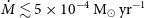 $\dot{M}\lesssim5\times10^{-4}\, \textrm{M}_{\odot} \,\textrm{yr}^{-1}$
, assuming a wind velocity of 50 km s
$\dot{M}\lesssim5\times10^{-4}\, \textrm{M}_{\odot} \,\textrm{yr}^{-1}$
, assuming a wind velocity of 50 km s
 $^{-1}$
. Using our derived mass-loss rate, and Equations A3 and A7 from Margutti et al. (Reference Margutti2018b), we estimate that this low-density environment occurs out to a distance of
$^{-1}$
. Using our derived mass-loss rate, and Equations A3 and A7 from Margutti et al. (Reference Margutti2018b), we estimate that this low-density environment occurs out to a distance of
 $R<3.7\times10^{15}$
cm.
$R<3.7\times10^{15}$
cm.
As NuSTAR observations showed that the source was X-ray bright in the hard X-ray band (Grefenstette et al. Reference Grefenstette, Brightman, Earnshaw, Harrison and Margutti2023), it is possible that SN2023ixf was emitting X-rays much earlier than the first Swift detection at 4.26 days after first light, but that the exposure time and sensitivity of the Swift observations were not sufficient to detect the highly-absorbed, high-temperature emission from the source. As such, if we perform the calculation above but instead use the time of the first Swift observation (1.57 days after first light) and its corresponding bolometric luminosity, we get
 $\dot{M}<3.1\times10^{-4}\,\textrm{M}_{\odot}\,\textrm{yr}^{-1}$
and
$\dot{M}<3.1\times10^{-4}\,\textrm{M}_{\odot}\,\textrm{yr}^{-1}$
and
 $R<1.8\times10^{15}$
cm.
$R<1.8\times10^{15}$
cm.
These results and those derived above are consistent with that calculated using our pre-explosion constraints and those published in the literature, including the mass-loss rates from Grefenstette et al. (Reference Grefenstette, Brightman, Earnshaw, Harrison and Margutti2023) using NuSTAR data and from Soraisam et al. (Reference Soraisam2023c) using the empirical period-luminosity-based mass-loss prescription from Goldman et al. (Reference Goldman2017). In addition, our shock radius is consistent with those derived by Grefenstette et al. (Reference Grefenstette, Brightman, Earnshaw, Harrison and Margutti2023), Smith et al. (Reference Smith2023), and Jacobson-Galan et al. (Reference Jacobson-Galan2023). However, our calculated mass-loss rate differs from other estimates in the literature, including that of Neustadt et al. (Reference Neustadt, Kochanek and Smith2023,
 $\sim$
 $10^{-5}$
 $\textrm{M}_\odot \, \textrm{yr}^{-1}$
), Niu et al. (Reference Niu2023,
$\textrm{M}_\odot \, \textrm{yr}^{-1}$
), Niu et al. (Reference Niu2023,
 $1 \times 10^{-5}$
 $\textrm{M}_\odot \, \textrm{yr}^{-1}$
], Bostroem et al. (Reference Bostroem2023,
$\textrm{M}_\odot \, \textrm{yr}^{-1}$
], Bostroem et al. (Reference Bostroem2023,
 $10^{-3}$
--
$10^{-3}$
--
 $10^{-2}$
 $\textrm{M}_\odot \, \textrm{ yr}^{-1}$
), Jacobson-Galan et al. (Reference Jacobson-Galan2023,
$\textrm{M}_\odot \, \textrm{ yr}^{-1}$
), Jacobson-Galan et al. (Reference Jacobson-Galan2023,
 $10^{-2}$
 $\textrm{M}_\odot \,\textrm{yr}^{-1}$
], and Hiramatsu et al. (Reference Hiramatsu2023a, 0.1 – 1
$\textrm{M}_\odot \,\textrm{yr}^{-1}$
], and Hiramatsu et al. (Reference Hiramatsu2023a, 0.1 – 1
 $\textrm{M}_\odot \, \textrm{yr}^{-1}$
(1–2 yr before explosion) and 0.1 – 1
$\textrm{M}_\odot \, \textrm{yr}^{-1}$
(1–2 yr before explosion) and 0.1 – 1
 $\textrm{M}_\odot \,\textrm{yr}^{-1}$
 $\sim$
(0.7-0.4 yr before explosion)). These discrepancies may be attributed to a number of factors including the chosen method or adopted parameters. For example, Niu et al. (Reference Niu2023) used the mass-loss rate prescription from Beasor & Davies (Reference Beasor and Davies2016) which relies on the progenitor mass, while Bostroem et al. (Reference Bostroem2023) and Jacobson-Galan et al. (Reference Jacobson-Galan2023) compared the spectroscopic evolution of SN2023ixf to a grid CMFGEN models that were sensitive to the adopted wind velocity,
$\sim$
(0.7-0.4 yr before explosion)). These discrepancies may be attributed to a number of factors including the chosen method or adopted parameters. For example, Niu et al. (Reference Niu2023) used the mass-loss rate prescription from Beasor & Davies (Reference Beasor and Davies2016) which relies on the progenitor mass, while Bostroem et al. (Reference Bostroem2023) and Jacobson-Galan et al. (Reference Jacobson-Galan2023) compared the spectroscopic evolution of SN2023ixf to a grid CMFGEN models that were sensitive to the adopted wind velocity,
 $v_w$
.
$v_w$
.
We can also use our best-fit hydrogen column density (
 $N_{H,hard}=(3.9_{-1.7}^{+1.2}\times10^{22}$
) cm
$N_{H,hard}=(3.9_{-1.7}^{+1.2}\times10^{22}$
) cm
 $^{-2}$
) to place a constraint on the mass loss, which yields a value consistent with Grefenstette et al. (Reference Grefenstette, Brightman, Earnshaw, Harrison and Margutti2023). Equation 4.1 from Fransson, Lundqvist, & Chevalier (Reference Fransson, Lundqvist and Chevalier1996) gives
$^{-2}$
) to place a constraint on the mass loss, which yields a value consistent with Grefenstette et al. (Reference Grefenstette, Brightman, Earnshaw, Harrison and Margutti2023). Equation 4.1 from Fransson, Lundqvist, & Chevalier (Reference Fransson, Lundqvist and Chevalier1996) gives
 \begin{equation} N_{H}=(2.1\times10^{22})\bigg(\frac{1}{\textrm{s}^{-1}}\bigg)\bigg(\frac{v_{w}}{10\, \textrm{km} \, \textrm{ s}^{-1}}\bigg)^{-1} \bigg(\frac{\dot{M}}{10^{-5}\,\textrm{M}_{\odot}}\bigg) \times \bigg(\frac{v_{s}}{10^{4}\, \textrm{km}\,\textrm{s}^{-1}}\bigg)^{1-s}\bigg(\frac{t}{8.90\, \textrm{days}}\bigg)^{1-s}\, \textrm{cm}^{-2},\end{equation}
where
 $N_{H}$
is the column density derived in Section 4.3, t is the time at which this column density was measured,
$N_{H}$
is the column density derived in Section 4.3, t is the time at which this column density was measured,
 $\dot{M}$
is the mass-loss rate,
$\dot{M}$
is the mass-loss rate,
 $v_{s}$
is the shock velocity as derived in Section 4.3,
$v_{s}$
is the shock velocity as derived in Section 4.3,
 $v_{w}=50$
km s
$v_{w}=50$
km s
 $^{-1}$
is the wind velocity, and
$^{-1}$
is the wind velocity, and
 $s=2$
is the index of the density profile. We find that the mass-loss rate of the progenitor was
$s=2$
is the index of the density profile. We find that the mass-loss rate of the progenitor was
 $(1.6_{-1.0}^{+0.9})\times10^{-4} \textrm{M}_{\odot}$
yr
$(1.6_{-1.0}^{+0.9})\times10^{-4} \textrm{M}_{\odot}$
yr
 $^{-1}$
, which is similar to both Grefenstette et al. (Reference Grefenstette, Brightman, Earnshaw, Harrison and Margutti2023) and what we derived above.
$^{-1}$
, which is similar to both Grefenstette et al. (Reference Grefenstette, Brightman, Earnshaw, Harrison and Margutti2023) and what we derived above.
Our derived shock radius suggests that the CSM of SN2023ixf is relatively compact. This is consistent with Grefenstette et al. (Reference Grefenstette, Brightman, Earnshaw, Harrison and Margutti2023), who measured a rapidly decreasing column density between their observations but also with the disappearance of CSM interaction signatures within 8 days of discovery (e.g. Jacobson-Galan et al. Reference Jacobson-Galan2023; Smith et al. Reference Smith2023) and the non-detection at millimeter wavelengths (Berger et al. Reference Berger2023a).
Assuming a constant shock velocity, we can use the ratio of the shock velocity (
 $\nu_{shock}$
) to the CSM velocity (or the wind velocity,
$\nu_{shock}$
) to the CSM velocity (or the wind velocity,
 $\nu_{wind}$
) and the time of observation (
$\nu_{wind}$
) and the time of observation (
 $t_{obs}$
) to place constraints on the pre-SN ejection time of the CSM (
$t_{obs}$
) to place constraints on the pre-SN ejection time of the CSM (
 $t_{ejection} $
) according to
$t_{ejection} $
) according to
 $t_{ejection} > t_{obs}(\nu_{shock}/\nu_{wind})$
from Dickinson et al. (Reference Dickinson2023). Using our derived mass-loss rate, the shock velocity derived in Section 4.3 and a wind velocity of 50 kms
$t_{ejection} > t_{obs}(\nu_{shock}/\nu_{wind})$
from Dickinson et al. (Reference Dickinson2023). Using our derived mass-loss rate, the shock velocity derived in Section 4.3 and a wind velocity of 50 kms
 $^{-1}$
, we find that SN2023ixf exhibited a mass-loss episode at least
$^{-1}$
, we find that SN2023ixf exhibited a mass-loss episode at least
 $ > 0.5-1.5 \, (v_{w}/50$
km s
$ > 0.5-1.5 \, (v_{w}/50$
km s
 $^{-1})$
yr prior to explosion. This is consistent with Jacobson-Galan et al. (Reference Jacobson-Galan2023), Kilpatrick et al. (Reference Kilpatrick2023), Jencson et al. (Reference Jencson2022), and Smith et al. (Reference Smith2023), who suggested that the progenitor experienced enhanced mass loss
$^{-1})$
yr prior to explosion. This is consistent with Jacobson-Galan et al. (Reference Jacobson-Galan2023), Kilpatrick et al. (Reference Kilpatrick2023), Jencson et al. (Reference Jencson2022), and Smith et al. (Reference Smith2023), who suggested that the progenitor experienced enhanced mass loss
 $ {>} $
1 yr prior to explosion.
$ {>} $
1 yr prior to explosion.
5.3 X-ray constraints on the CSM
In Fig. 12, we present our merged Swift X-ray spectrum with the best-fit models discussed in Section 4.3 and a model using the best-fit parameters (
 $N_{H}=5.6\times10^{22}$
cm
$N_{H}=5.6\times10^{22}$
cm
 $^{-2}$
and
$^{-2}$
and
 $kT=34$
keV) from epoch two (
$kT=34$
keV) from epoch two (
 $\sim$
11 days after first light) associated with the early NuSTAR data from Grefenstette et al. (Reference Grefenstette, Brightman, Earnshaw, Harrison and Margutti2023). While both our single-component models and the NuSTAR model describe the data equally well for energies
$\sim$
11 days after first light) associated with the early NuSTAR data from Grefenstette et al. (Reference Grefenstette, Brightman, Earnshaw, Harrison and Margutti2023). While both our single-component models and the NuSTAR model describe the data equally well for energies
 $>3$
keV, these models underestimate the emission at energies
$>3$
keV, these models underestimate the emission at energies
 $<2$
keV. We find that an additional low-temperature, absorbed bremsstrahlung component is able to reproduce the emission seen at energies
$<2$
keV. We find that an additional low-temperature, absorbed bremsstrahlung component is able to reproduce the emission seen at energies
 $<2$
keV.
$<2$
keV.
Similar to the well-studied Type IIn SN2010jl (Fransson et al. Reference Fransson2014; Chandra et al. Reference Chandra, Chevalier, Chugai, Fransson and Soderberg2015), we attribute this soft component to the cooling of the forward shock. Using the mass-loss constraint derived in Section 5.2.2 and the shock velocity derived from our high-temperature, bremsstrahlung component (see Section 4.3.2), we can calculate the cooling time. To do this we use Equation 6 from Fransson et al. (Reference Fransson2014):
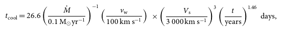 \begin{equation*}t_{\textrm{cool}} = 26.6 \left({\dot{M} \over 0.1\, \textrm{M}_{\odot} \textrm{yr}^{-1}}\right)^{-1} \left({v_{\textrm{w}} \over 100\, \textrm{km} \, \textrm{s}^{-1}}\right) \times \left({V_{\textrm{s}} \over 3\,000\, \textrm{km} \, \textrm{s}^{-1}}\right)^{3} \left( {t \over {\textrm{years}}}\right)^{1.46} \, \textrm{days},\end{equation*}
where
 $\dot{M}$
is the mass-loss rate,
$\dot{M}$
is the mass-loss rate,
 $v_{w}$
is the wind velocity,
$v_{w}$
is the wind velocity,
 $V_{s}$
is the shock velocity, and t is the time at which the mass-loss rate was measured. Assuming
$V_{s}$
is the shock velocity, and t is the time at which the mass-loss rate was measured. Assuming
 $v_w = 50 \, \, \textrm{km}\,\textrm{s}^{-1}$
,
$v_w = 50 \, \, \textrm{km}\,\textrm{s}^{-1}$
,
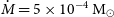 $\dot{M} = 5\times10^{-4}\, \textrm{M}_{\odot}$
yr
$\dot{M} = 5\times10^{-4}\, \textrm{M}_{\odot}$
yr
 $^{-1}$
,
$^{-1}$
,
 $V_{s}=5\,441 \, \, \textrm{km}\,\textrm{s}^{-1}$
, and
$V_{s}=5\,441 \, \, \textrm{km}\,\textrm{s}^{-1}$
, and
 $t\sim3.3$
days, we obtained a cooling time of
$t\sim3.3$
days, we obtained a cooling time of
 $t_{cool}\sim17$
days. Thus, it is possible that the forward shock is indeed cooling, giving rise to this additional component.
$t_{cool}\sim17$
days. Thus, it is possible that the forward shock is indeed cooling, giving rise to this additional component.
If we assume that the shock is propagating through a wind characterised by
 $\rho \propto R^{-2}$
, we would expect to see a decrease in the measured column density as the shock evolves, provided that the vast majority of the measured column density arises from CSM. As the Galactic absorption is much less than the measured column density derived in our analysis (
$\rho \propto R^{-2}$
, we would expect to see a decrease in the measured column density as the shock evolves, provided that the vast majority of the measured column density arises from CSM. As the Galactic absorption is much less than the measured column density derived in our analysis (
 $N_{H,gal}=7.9\times10^{20}$
cm
$N_{H,gal}=7.9\times10^{20}$
cm
 $^{-2}$
, HI4PI Collaboration et al. 2016), this is not an unreasonable assumption. In fact, the decrease in column density has been seen by both Grefenstette et al. (Reference Grefenstette, Brightman, Earnshaw, Harrison and Margutti2023) and Chandra et al. (2023b), who found a column density of
$^{-2}$
, HI4PI Collaboration et al. 2016), this is not an unreasonable assumption. In fact, the decrease in column density has been seen by both Grefenstette et al. (Reference Grefenstette, Brightman, Earnshaw, Harrison and Margutti2023) and Chandra et al. (2023b), who found a column density of
 $N_{H}=26\times10^{22}$
cm
$N_{H}=26\times10^{22}$
cm
 $^{-2}$
 $\sim$
4 days after first light, which decreased to
$\sim$
4 days after first light, which decreased to
 $N_{H}=5.6\times10^{22}$
cm
$N_{H}=5.6\times10^{22}$
cm
 $^{-2}$
on day
$^{-2}$
on day
 $\sim$
11 and then
$\sim$
11 and then
 $N_{H}\sim3.2\times10^{22}$
cm
$N_{H}\sim3.2\times10^{22}$
cm
 $^{-2}$
on day
$^{-2}$
on day
 $\sim$
14. Combined with our constraint of
$\sim$
14. Combined with our constraint of
 $3.9\times10^{22}$
cm
$3.9\times10^{22}$
cm
 $^{-2}$
by
$^{-2}$
by
 $\sim$
46 days, we find that the column density is decreasing following a simple power law with an index of
$\sim$
46 days, we find that the column density is decreasing following a simple power law with an index of
 $\sim$
 $1.5$
.
$1.5$
.
Figure 13. Unabsorbed X-ray luminosities (in units of
 $10^{41} \, \textrm{erg} \, \textrm{s}^{-1}$
) for SN2023ixf assuming a thermal bremsstrahlung model (0.3–10 keV, yellow stars) and other SNe detected in X-rays as a function of the time since first light (MJD=60082.83). Stars represent Type IIn SNe, while arrows indicate the measurement is an upper limit. For those SNe that are not Type IIn, the marker colour gives the SN type. Data Source and energy band: SN1970G (Immler & Kuntz Reference Immler and Kuntz2005, (0.3–2 keV)), SN1978K (Chandra Reference Chandra2018, (0.3–8 keV)), SN1980K (Schlegel Reference Schlegel2001, (2 keV)), SN1986J (Houck et al. Reference Houck, Bregman, Chevalier and Tomisaka1998, (0.5–2.2 keV)), SN1988Z (Schlegel & Petre Reference Schlegel and Petre2006, (0.2–2 keV)), SN1993J (Chandra et al. Reference Chandra, Dwarkadas, Ray, Immler and Pooley2009, (0.3–8 keV)), SN1994W (Chandra Reference Chandra2018, (0.3–8 keV)), SN1995N (Chandra et al. Reference Chandra, Ray, Schlegel, Sutaria and Pietsch2005, (0.1–10 keV)), SN1996cr (Chandra Reference Chandra2018, (0.5 - 2 keV)), SN1998bw (Kouveliotou et al. Reference Kouveliotou2004, (0.3–10 keV)), SN1998S (Pooley et al. Reference Pooley2002, (2–10 keV)), SN1999em (Schlegel Reference Schlegel2001, (2 keV)), SN1999gi (Schlegel Reference Schlegel2001, (2 keV)), SN2003bg (Soderberg et al. Reference Soderberg, Chevalier, Kulkarni and Frail2006, (0.5–8 keV)), SN2004et (Misra et al. Reference Misra2007, (0.5–8 keV)), SN2005kd (Chandra Reference Chandra2018, (0.3–8 keV)), SN2005ip (Katsuda et al. Reference Katsuda, Maeda, Nozawa, Pooley and Immler2014, (0.2–10 keV)), SN2006bp (Immler et al. Reference Immler2007, (0.2–10 keV)), SN2006gy (Chandra Reference Chandra2018, (0.5–2 keV)), SN2006jc (Immler et al. Reference Immler2008, (0.2–10 keV)), SN2006jd (Chandra Reference Chandra2018, (0.3–8 keV)), SCP06F6 (Levan et al. Reference Levan, Read, Metzger, Wheatley and Tanvir2013, (0.2–10 keV)), SN2008ax (Roming et al. Reference Roming2009, (0.2–10 keV)), SN2010jl (Chandra et al. Reference Chandra, Chevalier, Chugai, Fransson and Soderberg2015, (0.2–10 keV)), SN2011dh (Soderberg et al. Reference Soderberg2012, (0.3–8 keV)), SN2011fe (Margutti et al. Reference Margutti2012, (0.5–8 keV)), SN2014c (Brethauer et al. Reference Brethauer2022, (0.3–100 keV)), PTF12dam (Margutti et al. Reference Margutti2018a, (0.3–10 keV)), SN2017hcc (Chandra et al. Reference Chandra, Chevalier, James and Fox2022, (0.3–10 keV)),SN2018gk (Bose et al. Reference Bose2021, (0.3–10 keV)), SN2019ehk (Jacobson-Galán et al. Reference Jacobson-Galán2020, (0.3–10 keV)), SN2021gno (Jacobson-Galán et al. Reference Jacobson-Galán2022b, (0.3–10 keV)).
$10^{41} \, \textrm{erg} \, \textrm{s}^{-1}$
) for SN2023ixf assuming a thermal bremsstrahlung model (0.3–10 keV, yellow stars) and other SNe detected in X-rays as a function of the time since first light (MJD=60082.83). Stars represent Type IIn SNe, while arrows indicate the measurement is an upper limit. For those SNe that are not Type IIn, the marker colour gives the SN type. Data Source and energy band: SN1970G (Immler & Kuntz Reference Immler and Kuntz2005, (0.3–2 keV)), SN1978K (Chandra Reference Chandra2018, (0.3–8 keV)), SN1980K (Schlegel Reference Schlegel2001, (2 keV)), SN1986J (Houck et al. Reference Houck, Bregman, Chevalier and Tomisaka1998, (0.5–2.2 keV)), SN1988Z (Schlegel & Petre Reference Schlegel and Petre2006, (0.2–2 keV)), SN1993J (Chandra et al. Reference Chandra, Dwarkadas, Ray, Immler and Pooley2009, (0.3–8 keV)), SN1994W (Chandra Reference Chandra2018, (0.3–8 keV)), SN1995N (Chandra et al. Reference Chandra, Ray, Schlegel, Sutaria and Pietsch2005, (0.1–10 keV)), SN1996cr (Chandra Reference Chandra2018, (0.5 - 2 keV)), SN1998bw (Kouveliotou et al. Reference Kouveliotou2004, (0.3–10 keV)), SN1998S (Pooley et al. Reference Pooley2002, (2–10 keV)), SN1999em (Schlegel Reference Schlegel2001, (2 keV)), SN1999gi (Schlegel Reference Schlegel2001, (2 keV)), SN2003bg (Soderberg et al. Reference Soderberg, Chevalier, Kulkarni and Frail2006, (0.5–8 keV)), SN2004et (Misra et al. Reference Misra2007, (0.5–8 keV)), SN2005kd (Chandra Reference Chandra2018, (0.3–8 keV)), SN2005ip (Katsuda et al. Reference Katsuda, Maeda, Nozawa, Pooley and Immler2014, (0.2–10 keV)), SN2006bp (Immler et al. Reference Immler2007, (0.2–10 keV)), SN2006gy (Chandra Reference Chandra2018, (0.5–2 keV)), SN2006jc (Immler et al. Reference Immler2008, (0.2–10 keV)), SN2006jd (Chandra Reference Chandra2018, (0.3–8 keV)), SCP06F6 (Levan et al. Reference Levan, Read, Metzger, Wheatley and Tanvir2013, (0.2–10 keV)), SN2008ax (Roming et al. Reference Roming2009, (0.2–10 keV)), SN2010jl (Chandra et al. Reference Chandra, Chevalier, Chugai, Fransson and Soderberg2015, (0.2–10 keV)), SN2011dh (Soderberg et al. Reference Soderberg2012, (0.3–8 keV)), SN2011fe (Margutti et al. Reference Margutti2012, (0.5–8 keV)), SN2014c (Brethauer et al. Reference Brethauer2022, (0.3–100 keV)), PTF12dam (Margutti et al. Reference Margutti2018a, (0.3–10 keV)), SN2017hcc (Chandra et al. Reference Chandra, Chevalier, James and Fox2022, (0.3–10 keV)),SN2018gk (Bose et al. Reference Bose2021, (0.3–10 keV)), SN2019ehk (Jacobson-Galán et al. Reference Jacobson-Galán2020, (0.3–10 keV)), SN2021gno (Jacobson-Galán et al. Reference Jacobson-Galán2022b, (0.3–10 keV)).
This gradient is much steeper than expected assuming a steady, spherically symmetric wind (i.e. an index of 2). This could suggest that the source underwent either variable mass loss from the progenitor before explosion or the progenitor is surrounded by an intrinsically asymmetric CSM geometry (Fransson et al. Reference Fransson, Lundqvist and Chevalier1996) such as that seen in other interacting SN e.g. SN2006jd, SN2010jl, and SN1998S; Chandra et al. Reference Chandra2012; Fransson et al. Reference Fransson2014; Leonard et al. Reference Leonard, Filippenko, Barth and Matheson2000). The lack of pre-explosion outbursts (see Section 4.2, Neustadt et al. Reference Neustadt, Kochanek and Smith2023, Jencson et al. Reference Jencson2023, Dong et al. Reference Dong2023), and the evolution of the spectral features found in the high resolution spectra of SN2023ixf during its first week suggest that the CSM is likely asymmetric (e.g. Smith et al. Reference Smith2023), supporting the case that the observed decay in column density is largely due to the geometry of the CSM.
We can also derive the mass of the CSM swept up by the forward shock using the following (Chandra Reference Chandra2018; Margalit, Quataert, & Ho Reference Margalit, Quataert and Ho2022):
 $M_{CSM}=\dot{M}R_{s}(v_{w}/10\,$
km s
$M_{CSM}=\dot{M}R_{s}(v_{w}/10\,$
km s
 $^{-1})^{-1}$
. During the first
$^{-1})^{-1}$
. During the first
 $\sim46$
days, the shock had swept up
$\sim46$
days, the shock had swept up
 $\sim$
0.04–0.07
$\sim$
0.04–0.07
 $\textrm{M}_{\odot}$
of CSM. This is consistent with that estimated using optical spectra (Jacobson-Galan et al. Reference Jacobson-Galan2023; Bostroem et al. Reference Bostroem2023).
$\textrm{M}_{\odot}$
of CSM. This is consistent with that estimated using optical spectra (Jacobson-Galan et al. Reference Jacobson-Galan2023; Bostroem et al. Reference Bostroem2023).
5.4 Comparison with other X-ray bright SNe
SNe that explode in dense CSM are expected to be dominated by thermal X-ray emission from the forward shock with temperatures on the order of 10 to a few 10s of keV (e.g. see review by Chandra Reference Chandra2018). The increase in X-ray emission seen from SN2023ixf indicates that its shock is interacting with a dense, hydrogen-rich CSM that was recently ejected by the progenitor prior to its death. This is consistent with our results presented in Section 4.3.2 and the growing body of evidence that pre-explosion mass loss occurs in the progenitors of Type IIn-like SNe through either binary interaction or episodic mass loss (e.g. see review by Smith Reference Smith2014).
In Fig. 13, we plot our X-ray luminosity as a function of time for SN2023ixf assuming a thermal bremsstrahlung model and compare it to a sample of other X-ray bright SNe. The rise in the X-ray emission of SN2023ixf (Fig. 11, lower left panel) has been seen in a number of interacting SNe including Type IIn SN2010jl (Chandra et al. Reference Chandra, Chevalier, Chugai, Fransson and Soderberg2015) and SN2006jd (Chandra Reference Chandra2018), and the Type Ib SN2014c that transitioned into a strongly interacting Type IIn (Margutti et al. Reference Margutti2017; Thomas et al. Reference Thomas2022). However, the timescales to peak X-ray brightness for these other events are much longer (
 $\sim$
100 days) compared to the
$\sim$
100 days) compared to the
 $\sim$
10 days it took for the soft X-rays from SN2023ixf to attain their current peak. This difference in rise time is likely due to the location of the CSM, with the CSM surrounding SN2023ixf likely more compact compared to the other SNe that show interaction or which emit X-rays (Fig. 13). This rise in X-ray brightness is also likely a result of the decrease in shock temperature as it sweeps and interacts with more material over time. This causes the X-ray emission to shift from higher to lower X-rays energies. Such behaviour is consistent with the decrease in shock temperature seen by NuSTAR (Grefenstette et al. Reference Grefenstette, Brightman, Earnshaw, Harrison and Margutti2023). The flattening in the X-ray light curve seen after
$\sim$
10 days it took for the soft X-rays from SN2023ixf to attain their current peak. This difference in rise time is likely due to the location of the CSM, with the CSM surrounding SN2023ixf likely more compact compared to the other SNe that show interaction or which emit X-rays (Fig. 13). This rise in X-ray brightness is also likely a result of the decrease in shock temperature as it sweeps and interacts with more material over time. This causes the X-ray emission to shift from higher to lower X-rays energies. Such behaviour is consistent with the decrease in shock temperature seen by NuSTAR (Grefenstette et al. Reference Grefenstette, Brightman, Earnshaw, Harrison and Margutti2023). The flattening in the X-ray light curve seen after
 $\sim$
10 days (See Fig. 11 lower left panel) suggests that the X-ray emission is currently powered by CSM interaction. This behaviour has been seen in both SN2014c and other Type IIn SNe with well-sampled X-ray light curves (e.g. SN2010jl Chandra et al. Reference Chandra, Chevalier, Chugai, Fransson and Soderberg2015, SN2006jd Chandra et al. Reference Chandra2012 and see Fig. 13).
$\sim$
10 days (See Fig. 11 lower left panel) suggests that the X-ray emission is currently powered by CSM interaction. This behaviour has been seen in both SN2014c and other Type IIn SNe with well-sampled X-ray light curves (e.g. SN2010jl Chandra et al. Reference Chandra, Chevalier, Chugai, Fransson and Soderberg2015, SN2006jd Chandra et al. Reference Chandra2012 and see Fig. 13).
Compared to other Type IIn SNe, both the bolometric luminosity (see Fig. 6) and the X-ray luminosity of SN2023ixf (see Fig. 13) are currently a few orders of magnitude less than that seen for strongly interacting SNe such as SN2010jl (Chandra et al. Reference Chandra, Chevalier, Chugai, Fransson and Soderberg2015), SN2006jd (Chandra et al. Reference Chandra2012), and SN2005kd (Dwarkadas et al. Reference Dwarkadas, Romero-Cañizales, Reddy and Bauer2016), and is more consistent in luminosity with that seen from Type IIn SN2006gy (Smith et al. Reference Smith2007), SN1998S (Pooley et al. Reference Pooley2002), SN2017hcc (Chandra et al. Reference Chandra, Chevalier, James and Fox2022), or some Type IIP, Type IIb, or Type Ib SNe. The low X-ray luminosity of SN2023ixf is rather peculiar given: that Type IIn SNe tend to be much brighter in X-rays than other core-collapse SNe (e.g. Chandra Reference Chandra2018), that the shock appears to be interacting with dense material based on flash ionisation features (e.g. Jacobson-Galan et al. Reference Jacobson-Galan2023; Smith et al. Reference Smith2023; Jencson et al. Reference Jencson2023), the constraints on the CSM both in this work and others in the literature, the enhanced mass-loss rates derived in this and in other works, and the large column densities relative to the Galactic column density measured here and by NuSTAR (Grefenstette et al. Reference Grefenstette, Brightman, Earnshaw, Harrison and Margutti2023) and Chandra (Chandra et al. Reference Chandra, Maeda, Chevalier, Nayana and Ray2023b).
Similar to the Type IIn SN SN2017hcc, which exhibited weak X-ray and radio emission but bright IR emission, it is possible that SN2023ixf’s low-luminosity X-ray emission arises from an asymmetric CSM. In this case, the conversion of kinetic energy is inefficient in some directions, causing a lower X-ray flux. Another possibility is that the X-ray emission is suppressed due to instabilities at the shock front or due to the hot post-shock gas driving weak shocks into the colder surrounding material, transferring energy before it can be radiated (e.g. Steinberg & Metzger Reference Steinberg and Metzger2018). As a number of studies in the literature suggest that the CSM is asymmetric (e.g. Smith et al. Reference Smith2023; Berger et al. Reference Berger2023b; Vasylyev et al. Reference Vasylyev2023), it is likely the lower X-ray luminosity is a signature of the CSM distribution.
We can expect that once the X-ray luminosity begins to fade, it will decay following
 $t^{-1}$
if the CSM was formed via a steady wind whose density decreases as
$t^{-1}$
if the CSM was formed via a steady wind whose density decreases as
 $r^{-2}$
(e.g. Chevalier Reference Chevalier1998; Dwarkadas & Gruszko Reference Dwarkadas and Gruszko2012). However, it has been shown that a number of SNe that are known to interact with a dense CSM deviate from this behavior (see e.g. Dwarkadas & Gruszko Reference Dwarkadas and Gruszko2012; Ross & Dwarkadas Reference Ross and Dwarkadas2017; Chandra Reference Chandra2018). This could result from either a CSM that does not follow
$r^{-2}$
(e.g. Chevalier Reference Chevalier1998; Dwarkadas & Gruszko Reference Dwarkadas and Gruszko2012). However, it has been shown that a number of SNe that are known to interact with a dense CSM deviate from this behavior (see e.g. Dwarkadas & Gruszko Reference Dwarkadas and Gruszko2012; Ross & Dwarkadas Reference Ross and Dwarkadas2017; Chandra Reference Chandra2018). This could result from either a CSM that does not follow
 $r^{-2}$
(Salamanca Reference Salamanca, Perez, Gonzalez Delgado and Tenorio-Tagle2003; Dwarkadas Reference Dwarkadas2011; Dwarkadas & Gruszko Reference Dwarkadas and Gruszko2012), or from the fact that our X-ray instruments observe in a narrow X-ray band (Dwarkadas & Gruszko Reference Dwarkadas and Gruszko2012) and thus our bolometric corrections are not capturing the full emission. As our analysis suggests that the CSM was formed from low-luminosity, episodic mass loss or from binary interaction, we expect that the emission will decay following a power law that deviates from this behaviour. As such, it will be critical to continue monitoring the X-ray evolution of SN2023ixf as it evolves to further probe the mass-loss history of its stellar progenitor.
$r^{-2}$
(Salamanca Reference Salamanca, Perez, Gonzalez Delgado and Tenorio-Tagle2003; Dwarkadas Reference Dwarkadas2011; Dwarkadas & Gruszko Reference Dwarkadas and Gruszko2012), or from the fact that our X-ray instruments observe in a narrow X-ray band (Dwarkadas & Gruszko Reference Dwarkadas and Gruszko2012) and thus our bolometric corrections are not capturing the full emission. As our analysis suggests that the CSM was formed from low-luminosity, episodic mass loss or from binary interaction, we expect that the emission will decay following a power law that deviates from this behaviour. As such, it will be critical to continue monitoring the X-ray evolution of SN2023ixf as it evolves to further probe the mass-loss history of its stellar progenitor.
6. Summary and conclusions
We have presented a comprehensive study of the pre-explosion UV, optical, and X-ray properties, and post-explosion X-ray emission of the nearby Type IIn SN SN2023ixf as detected by Swift, ASAS-SN, ATLAS, ZTF, Chandra, and XMM-Newton. Here, we analysed data from nearly two decades prior to explosion and
 $\sim$
50 days post explosion, focusing on the pre-explosion variability, presence of X-ray signatures prior to explosion and the evolution of the luminous soft X-ray emission. In summary:
$\sim$
50 days post explosion, focusing on the pre-explosion variability, presence of X-ray signatures prior to explosion and the evolution of the luminous soft X-ray emission. In summary:
-
1. Using nearly two decades of data, we showed that the progenitor of SN2023ixf exhibited no significant evidence of pre-explosive/precursor activity in the optical, UV, and X-rays as detected by Swift, ASAS-SN, ZTF, ATLAS, Chandra, and XMM-Newton. This is consistent with that found by Neustadt et al. (Reference Neustadt, Kochanek and Smith2023)), Hiramatsu et al. (Reference Hiramatsu2023a) and Dong et al. (Reference Dong2023). Our analysis suggests that any evidence of precursor activity in optical to UV was characterised by a luminosity
 $\lesssim$
$1\times10^{5} \, \textrm{L}_{\odot}$
, consistent with Neustadt et al. (Reference Neustadt, Kochanek and Smith2023), Jencson et al. (Reference Jencson2023), and Dong et al. (Reference Dong2023) who suggested that there was no bright, short-lived outburst within the last
$\sim$
decades prior to explosion.
$\lesssim$
$1\times10^{5} \, \textrm{L}_{\odot}$
, consistent with Neustadt et al. (Reference Neustadt, Kochanek and Smith2023), Jencson et al. (Reference Jencson2023), and Dong et al. (Reference Dong2023) who suggested that there was no bright, short-lived outburst within the last
$\sim$
decades prior to explosion. -
2. Extensive, serendipitous monitoring of the location of SN2023ixf by Chandra, Swift, and XMM-Newton prior to explosion shows no evidence of luminous precursor emission down to 5.7
$\times10^{36}$
erg s
$^{-1}$
based on Chandra observations spanning more than 18 yr prior to the explosion. Using Swift observations from the progenitor’s final 16 yr, we instead obtain a value of less than 5.8
$\times10^{37}$
erg s
$^{-1}$
and derive a mass-loss rate of
$(3-10)\times10^{-5} \textrm{M}_{\odot}$
yr
$^{-1}$
, which is consistent with those rates derived by Neustadt et al. (Reference Neustadt, Kochanek and Smith2023) and Jencson et al. (Reference Jencson2023). -
3. Using the extensive set of Swift XRT observations of SN2023ixf that have been taken since its discovery, we find that Swift did not detect any soft X-ray emission down to an unabsorbed luminosity of
$7.2\times10^{38}$
erg s
$^{-1}$
within the first
$\sim$
$3.3$
days after first light. Assuming that the emission is dominated by IC scattering, similar to that done for other SNe (e.g. Margutti et al. 2012, 2014), we derive a mass-loss rate of
$\lesssim$
$5\times10^{-4} \textrm{M}_{\odot}$
yr
$^{-1}$
and a radius of
$R<3.7\times10^{15}$
cm for the CSM. Our analysis suggests that the progenitor underwent a mass-loss episode at least
$ > 0.5-1.5 (v_{w}/50$
km s
$^{-1})$
yr prior to explosion. -
4. By merging the available Swift XRT observations, we find that the emission over the first
$\sim$
50 days is best described by an absorbed, two-temperature component bremsstrahlung model. Here, the hard component has a temperature of
$\sim$
35 keV and a column density of
$3.9\times10^{22}$
cm
$^{-2}$
, consistent with that found using NuSTAR (Grefenstette et al. Reference Grefenstette, Brightman, Earnshaw, Harrison and Margutti2023). The soft component has a temperature of
$\sim$
$0.3$
keV and a column density of
$0.9\times10^{22}$
cm
$^{-2}$
, which we suggest results from the forward shock cooling, similar to that seen in SN2010jl. We also derive a swept up mass of 0.04–0.07
$\textrm{M}_{\odot}$
for the CSM. -
5. Similar to other interacting SNe, we find that the X-ray emission of SN2023ixf has risen to peak brightness and is now plateauing. However, the rise to peak was much faster than other interacting SNe, while the peak luminosity is nearly a few orders of magnitude less than that seen for strongly interacting SNe such as SN2010jl or SN2006jd. This is peculiar considering the fact that SN2023ixf showed evidence of flash ionisation features and enhanced mass-loss rates. We suggest that the low X-ray luminosity may be a natural consequence of an asymmetric CSM, similar to that of the Type IIn SN 2017hcc and consistent with the findings of Smith et al. (Reference Smith2023), Berger et al. (Reference Smith2023b), and Vasylyev et al. (Reference Vasylyev2023).


Due to its proximity and extensive pre- and post-explosion multiwavelength coverage, SN2023ixf provides a unique opportunity to not only understand the time-dependent mass loss, variability and CSM formation associated with the final stages of red supergiant evolution but also the possible effects of binarity on these systems. The continued monitoring of the electromagnetic emission (in addition to neutrinos and gravitational waves) from SN2023ixf will provide some of the strongest constraints on the mechanism associated with stellar collapse of a massive progenitor seen in the last few decades.
Acknowledgement
We thank C. Kochanek for his insight and advice.
Funding statement
Parts of this research were conducted by the Australian Research Council Centre of Excellence for Gravitational Wave Discovery (OzGrav), through project number CE170100004.
LAL acknowledges support by the Simons Foundation and the Heising-Simons Foundation. This work was performed in part at the Simons Foundation Flatiron Institute’s Center for Computational Astrophysics during LAL’s tenure as an IDEA Scholar.
JFB was supported by National Science Foundation grant No. PHY-2310018.
Data availability
Not applicable.
Appendix
In Table A1, we present the results of our variability analysis as outlined in Section 4.2.
Table A1. Variability Limits for SN2023ixf in various bands.
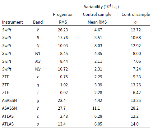


 Open access