


Introduction
Nanosphere lithography (NSL) provides a cost-effective method to fabricate periodic nanopatterns on large surface areas (Hulteen & Van Duyne, Reference Hulteen and Van Duyne1995; Boneberg et al., Reference Boneberg, Burmeister, Schäfle and Leiderer1997; Haginoya et al., Reference Haginoya, Ishibashi and Koike1997; Burmeister et al., Reference Burmeister, Badowsky, Braun, Wieprich, Boneberg and Leiderer1999). Regular arrays have a great potential for applications, for example, in optoelectronics (Sim et al., Reference Sim, Lee, Yang, Yoon and Kim2011; Zhang et al., Reference Zhang, Yang, Wang, Fu, Wang, Long and Lu2013), electrochemical sensors (Purwidyantri et al., Reference Purwidyantri, Chen, Hwang, Luo, Chiou, Tian, Lin, Cheng and Lai2016), optical fiber tip nanoprobes (Pisco et al., Reference Pisco, Galeotti, Quero, Grisci, Micco, Mercaldo, Veneri, Cutolo and Cusano2017), and as metamaterials (Gwinner et al., Reference Gwinner, Koroknay, Fu, Patoka, Kandulski, Giersig and Giessen2009). Recently, it has been demonstrated that NSL masks can be fabricated in roll-to-roll processes, opening the path to industrial scale applications (Chen et al., Reference Chen, Schappell, Zhang and Chang2020). Often, a narrow size distribution of the nanoobjects is desired in order to realize devices with well-defined emission or absorption properties (Haynes & Van Duyne, Reference Haynes and Van Duyne2001; Qian et al., Reference Qian, Li, Wasserman and Goodhue2008). Therefore, it is important to determine the factors governing the size distribution of the nanoscale openings in the sphere monolayers or double layers, which serve as lithographic masks. In case of close-packed monolayer masks, the mask openings, also referred to as interstices, are defined by sphere triples.
Up to now, the mask opening size distribution has been investigated only indirectly by analyzing atomic force microscopy or scanning electron microscopy (SEM) images of nanoparticle arrays fabricated by physical vapor deposition through sphere layer masks (Hulteen & Van Duyne, Reference Hulteen and Van Duyne1995; Hulteen et al., Reference Hulteen, Treichel, Smith, Duval, Jensen and Van Duyne1999; Li & Zinke-Allmang, Reference Li and Zinke-Allmang2002; Riedl & Lindner, Reference Riedl and Lindner2014). Li & Zinke-Allmang found that the size distribution of Ge particles deposited at the interstices of a polystyrene sphere monolayer is broader than that of the spheres, and ascribed the difference to packing imperfections of the spheres (Li & Zinke-Allmang, Reference Li and Zinke-Allmang2002). Hulteen et al. studied the size distributions of Ag nanoparticles obtained at the openings of polystyrene sphere mono- and double layers (Hulteen et al., Reference Hulteen and Van Duyne1999). The authors conclude that the standard deviation of the interstice size roughly equals that of the sphere diameter. However, if the sphere size variation was the only cause for the interstice size distribution, the coefficient of variation (CV) of the interstice size would be given by the CV of the average sphere diameters of the groups of three spheres (i.e., sphere triples) defining an interstice. In other words, the standard deviation of the interstice size would be significantly smaller than that of the sphere diameter. The reasons for this are two-fold: First, since the average diameter of the spheres in a triple determines the interstice size as a first approximation, sphere diameter differences level out partially, that is, the standard deviation of the average diameters of the spheres in a triple is smaller than that of the sphere diameters by a factor of 31/2. Second, the sphere diameter D is linearly interrelated to the interstice equivalent diameter D eq,is, that is, the diameter of a circle with the same area as the interstice area (see Supplementary Section 1.1):
 $$D_{{\rm eq, is}} = \left({\displaystyle{{3^{1/2}} \over \pi }-\displaystyle{1 \over 2}} \right)^{1/2}\cdot D\approx 0.227\cdot D, \;$$
with a proportionality factor < 1.
Thus, the experimentally observed larger CV of the interstice size as compared to the CV of the average sphere diameters of the triples indicates that there must exist further sources of size broadening. To the best of our knowledge, a direct analysis of the mask opening size distribution and of its geometric origins such as the sphere diameter distribution, sphere position variations and interstice corner rounding/filling due to surface energy minimization or deposition of solutes from the sphere suspension has not yet been made.
To analyze the size of the mask openings together with that of the spheres forming them, the individual spheres and triples of them have to be identified in the image. In order to detect nearly spherical objects corresponding to circles in the image, several methods are reported in the literature: Circle Hough transformation and its variants (Duda & Hart, Reference Duda and Hart1975; Scaramuzza et al., Reference Scaramuzza, Pagnottelli and Valigi2005), the random sample consensus algorithm (Götzinger, Reference Götzinger2015), correlation-based template matching (Ceccarelli et al., Reference Ceccarelli, Petrosino and Laccetti2001), marker-based watershed segmentation (Gostick, Reference Gostick2017), and region-based convolutional neuronal networks (Girshick et al., Reference Girshick, Donahue, Darrell and Malik2014). While these techniques have enabled a remarkable progress in the detection of spherical objects, they also exhibit shortcomings. In the case of high-resolution SEM images of sphere monolayers, the sphere objects are partly interconnected in a nearly regular array containing defects. Due to the concomitant image intensity variations, in addition to noise, this can complicate the complete capture of the sphere edges, and thus lower the accuracy of the analysis, as well as give rise to false negative and false positive detection events. In our contribution, we develop an automated analysis procedure based on intensity profiling and cross-correlation, which is capable of quantifying the sphere diameters, the sizes of sphere triple interstices and sphere positions. The method is applied to widely used monodisperse polystyrene sphere monolayer masks with sphere diameters between 220 and 600 nm. In particular, the correlation between the evaluated quantities is assessed, and the relative importance of the factors leading to the observed interstice size distribution widths is determined. This knowledge will help identifying the materials and conditions favorable for obtaining ultra-narrow mask opening and thus nanostructure size distributions.
Materials and Methods
The experimental procedure used consists of a cleaning and hydrophilization treatment of Si wafer pieces, followed by the deposition of polystyrene sphere monolayers and then imaging in a scanning electron microscope. Rectangular pieces (4 cm × 2 cm) were cut from a 4-inch n-doped Si (001) wafer. After cleaning the surface by rinsing with deionized H2O and isopropyl alcohol, the wafer pieces were hydrophilized by an O2/Ar plasma treatment (2 sccm O2, 8 sccm Ar, pressure 10 Pa, RF power 50 W, duration 3 min) in a Plasmalab 80plus machine (Oxford Instruments). The hydrophilicity was checked by means of optical measurements of the contact angle of deionized H2O droplets placed on the wafer surface using a Drop Shape Analyzer DSA25E (Krüss company).
Next, monolayers of monodisperse polystyrene spheres with three different sphere sizes, 220, 370, and 600 nm were deposited from aqueous suspensions (10 wt% solids, Thermo Fisher Scientific Inc.) on the hydrophilized Si substrate by means of the doctor blade technique (Kumnorkaew et al., Reference Kumnorkaew, Ee, Tansu and Gilchrist2008; Riedl & Lindner, Reference Riedl and Lindner2014). A drop of the colloidal suspension is pipetted onto the substrate surface, brought into contact with a blade and then moved at a constant velocity across the surface (Fig. 1). At the three-phase contact line between the substrate, the suspension and the gas atmosphere two-dimensional close-packed sphere layers form due to the action of attractive capillary forces between the spheres and the convective stream of suspension toward the three-phase line (Dimitrov et al., Reference Dimitrov, Dushkin, Yoshimura and Nagayama1994; Kumnorkaew et al., Reference Kumnorkaew, Ee, Tansu and Gilchrist2008). In order to obtain sphere monolayers a suitable blade velocity was chosen, which depends on sphere size, temperature, and atmosphere humidity. The resulting sphere layers were imaged in a field emission SEM electron beam lithography system (Raith Pioneer) at 5 kV using an inlens detector.

Fig. 1. Schematic cross-section view of the formation of colloidal monolayers at the three-phase contact line in the doctor blade technique.  $j_{{\rm H}_ 2{\rm O}}$, j P, and j e denote the liquid H2O, solid sphere particle, and H2O evaporation fluxes.
Image Analysis Method
In this section, the individual image processing and evaluation steps are described. All steps are implemented in a script developed for the Gatan DigitalMicrograph software (GMS 2, 2014). The script is available in the DigitalMicrograph Script Database hosted by FELMI, Graz University of Technology (FELMI, 2021). As input data, unprocessed SEM images of sphere monolayers are used, which should have (i) sufficient spatial resolution and pixel density in order to clearly resolve the sphere outlines, (ii) a sufficient signal-to-noise ratio, and (iii) sufficient contrast between the spheres and their interstices. Recommended values are listed in Table 1. For statistical analyses, the image area should cover several hundreds of spheres. The typical image size is 2,000 to 3,000 pixels in each dimension. An example of such an SEM image of a particularly defective sphere monolayer is given in Figure 2. Numerous line defects in the sphere arrangement and various mask defects involving overly small spheres are visible. Line defects appear brighter in the image since the spheres bordering the line charge up electrically, leading to a locally enhanced secondary electron emission. This example is chosen to demonstrate the robustness of the image analysis method developed in the following section.

Fig. 2. Raw SEM image of a sphere monolayer showing more than 500 spheres with an average diameter of 220 nm.
Table 1. Quality Parameters of SEM Images of Sphere Monolayers Recommended for the Automated Analysis.

a Signal = intensity difference between the interstice and adjacent sphere interiors.
b Contrast = intensity difference between the interstice and adjacent sphere interiors divided by the mean intensity of the same interstice and sphere interiors.
c Averaged over the entire image.
Filtering and Average Correction
At the beginning of image analysis, two preparatory steps are performed. First, in order to minimize noise, the raw image is smooth-filtered by convolution in real space using a filter kernel. Each pixel is replaced by a weighted sum of its surrounding pixels. The array of weights for each of the surrounding pixels forms the kernel  ${\bf K}$. Here, the kernel
 $${\bf K} = \matrix{ 1 & 2 & 1 \cr 2 & 4 & 2 \cr 1 & 2 & 1 \cr } $$
implemented in the “smooth” menu command of the DigitalMicrograph software is used. In this kernel, the center pixel has fourfold weight, whereas the central top, bottom, left, and right pixels have double, and the corner pixels single weight.
Second, a local average-corrected image I corr(x, y) is computed from the smooth-filtered image I sm(x, y), in order to reduce large-scale intensity variations due to differences in the secondary electron emission rate between the perfect crystalline areas and the zones containing defects:
 $$I_{{\rm corr}}( x, \;y) = \displaystyle{{I_{{\rm sm}}( x, \;y) } \over {I_{{\rm avg}}( x, \;y) }}\cdot \bar{I}.$$ $\bar{I}$ denotes the mean image intensity in the entire image and
 $$I_{{\rm avg}}( x, \;y) = \displaystyle{{\sum\limits_{y^{\prime} = y-b{\rm /}2}^{y + b{\rm /}2} {\sum\limits_{x^{\prime} = x-b{\rm /}2}^{x + b{\rm /}2} {I_{{\rm sm}}( x^{\prime}, \;y^{\prime}) } } } \over {b^2}}$$
the local average intensity image, which is obtained by assigning to each pixel (x, y) the average intensity of a square region of interest (ROI) of size b (with b = even integer and b ≈ 40% of the average sphere diameter) centered at (x, y). The loop variables x′, y′ are confined inside the image boundaries. Figure 3 depicts the average-corrected image of the SEM image in Figure 2.

Fig. 3. Smooth-filtered and average-corrected version of the SEM image in Figure 2.
Taking the local average-corrected image as input, the sphere detection is achieved in three steps. In step 1, seed spheres are detected (20–30% of all spheres), followed by the detection of the large majority of spheres in step 2 and a search optimized for spheres of deviating size in step 3. All three steps include fitting circles to the sphere circumferences.
Seed Sphere Detection
Seed sphere detection starts with the preselection of possible sphere positions by defining a grid of square ROIs (ROI size: 1.3 times the sphere diameter D) on the image. Each ROI is then cross-correlated with an equally sized reference image of a fully six-fold coordinated sphere, which is taken from the image at a position specified by the user. If the distance between the detected position of the correlation maximum and the ROI center is below a threshold value of D/3 (determined from test runs), an ROI of the same size centered at the correlation maximum is examined by means of an intensity profiling module. This module extracts intensity profiles along lines inclined by various angles centered at the correlation maximum position (Figs. 4a, 4b). Typically, 18 profiles are extracted using equidistant angular steps. In order to minimize the intensity scatter, the profiles have a width of a few pixels (not shown in Fig. 4a). Next, intensity steps with sufficient height and not too large width are searched in these profiles in order to determine the edges of the sphere. If these intensity steps (i) either have positive sign and are situated in the first profile half, or have negative sign and occur in the second profile half, and if (ii) the distance between two such steps of opposite sign lies within the interval
 $$Intvl = [ {( 1-k_1) \overline D ; \;( 1 + k_2) \overline D } ] , \;$$
with k 1 = k 2 = 0.2 and  $\overline D$ is an approximate estimate of the average sphere diameter (input by the user), then the step positions are recognized as points on the sphere circumference, that is, sphere edge points (Fig. 4c). The restriction for the separation of two steps of opposite sign helps to minimize the detection of false positions. If more than a user-defined number of edge points (typically 16 for 18 profiles) are found, a circle is fitted to them by means of an iterative procedure (Fig. 4d). In case of a sufficiently high fit quality (measured as the sum of squared distances between circle and edge points, normalized to the number of points), the fitted position is accepted as a sphere center position. Figure 5 depicts the SEM image with all 133 detected seed spheres marked.

Fig. 4. (a) Enlarged subarea of the SEM image of Figure 3 with a marked example position and the corresponding 18 intensity profile lines, (b) the intensity profile marked by a star in (a), (c,d) same image subarea as in (a) with (c) marked sphere edge points and (d) fitted circle line and center position. The length bar is 100 nm in (a,c,d).

Fig. 5. SEM image of Figure 3 with 133 fitted seed spheres. The fitted spheres are highlighted as dark grey areas with the center positions marked as white dots.
Sphere Detection Step 2
In contrast to the raster search for the seed spheres, the detection algorithms used in step 2 to find the large majority of spheres rely on combined star and 360° searches. The star search works most effectively in case of perfect monocrystalline sphere arrangements. The name of this search reflects the six different search directions along the close-packed directions in the 2D lattice starting out from the seed sphere positions. For the determination of these directions, the angular positions of the maxima in the Fourier transforms of ROIs are evaluated, where the ROIs are centered at the positions of the seed spheres (Figs. 6a, 6b). In this way, new potential sphere positions in the first nearest-neighbor shell are identified at a distance to the seed sphere that equals the estimated average sphere diameter. In addition, further 54 potential positions are identified in the second, third, and fourth nearest-neighbor shells by assuming the spheres to sit on regular positions of the close-packed 2D lattice (Fig. 6c). Analogously to the seed sphere detection procedure, the positions are refined by means of cross-correlation, then subjected to the intensity profiling (see Section “Seed sphere detection”), sphere edge point detection and fitting routines described above. As the star search assumes a perfect lattice, it often does not recognize spheres located at defects occurring in the sphere monolayers, namely small gaps between neighboring spheres, line defects and small zones with reduced sphere coordination. Therefore, a 360° search has been developed, which is suitable for disordered sphere arrangements with 1–6 nearest neighbors. Here, the cross-correlation between the reference sphere image and image ROIs centered at a fixed distance (estimated sphere diameter) from the seed sphere center is evaluated as a function of the azimuth angle (Figs. 7a, 7b). The positions with maximum correlation are then selected for the subsequent intensity profiling, edge point, and fitting operations, as described above. In order to include positions further away from the seed sphere, the 360° search has been programmed as an endless routine, that is, it is repeated taking the newly detected position as starting position. The process continues as long as further not yet detected nearest-neighbor spheres are recognized inside the image boundaries. As illustrated in Figure 8, the combined star and 360° searches are capable of detecting around 99% of the spheres (seed spheres included, image border regions excluded).

Fig. 6. Star sphere search: (a) subarea of the SEM image of Figure 3; the square marks the area used for the Fourier transformation. (b) Central part of the Fourier transform magnitude image computed from the marked area in (a). In (a), (b) and (c), the close-packed direction is highlighted that belongs to the most-intense off-center Fourier peak. For the purpose of finding this peak, the central Fourier maximum has been removed. (c) Detected lattice positions corresponding to the sphere arrangement of (a), which are proposed as potential sphere positions. The seed sphere is marked with a small blue circle.

Fig. 7. 360° sphere search: (a) subarea of the SEM image of Figure 3; the central seed sphere and the nearest-neighbor sphere displaying the largest cross-correlation are marked in violet and orange, respectively. (b) Maximum values of the cross-correlation images plotted as a function of the azimuth angle. The cross-correlation images are computed from the reference sphere image and image ROIs positioned at variable azimuth angle at a constant distance to the seed sphere center (the red dotted circle line). In (a, and (b), the colored dashed lines mark the directions or angular positions that correspond to the cross-correlation maxima in plot (b).

Fig. 8. SEM image of Figure 3 with 519 marked fitted spheres, which have been detected in course of the sphere searches of step 1 (seed spheres) and step 2 (combined star and 360° searches).
Detection of Spheres of Deviating Size
As the sphere search steps 1 and 2 are designed for average-sized spheres, spheres of deviating size, in the present case mostly significantly smaller spheres, are often overlooked. To include these spheres with diameters significantly below the average, a third search step is conducted. In this step, potential sphere positions outside the fitted circles of the before detected spheres are identified. These positions are examined by using intensity profiling and a modified sphere edge point detection routine which is opened for a wider range of sphere diameters by choosing appropriate values for k 1 and k 2 in equation (5). The fitting is performed as described in steps 1 and 2. Overall, at least 99.8% of all spheres are detected (image border regions excluded), and accurate fit results for their center positions and diameters obtained (Fig. 9). Based on these data, the sphere diameter histogram and statistical key figures such as average, standard deviation, and CV are evaluated.

Fig. 9. SEM image of Figure 3 with 525 marked fitted spheres, which have been detected in course of the sphere searches of steps 1–3.
Identification of Sphere Triples
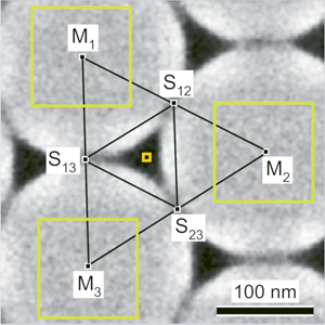
Based on the analysis described before, another module of the program identifies the sphere triples as a preparatory step for the interstice size evaluation. By sphere triples we mean sets of three spheres, where each of the three spheres forms a contact to the other two spheres. The triple identification is performed by means of intensity profile analyses. For each two spheres with separation
 $$s = \overline {{\rm M}_ 1{\rm M}_ 2} -R_1-R_2$$
( $\overline {{\rm M}_ 1{\rm M}_ 2}$ is the distance between the sphere centers M1, M2; R 1, R 2 are fitted sphere radii) below a threshold value, the M1M2 center-to-center profile and the profile perpendicular to M1M2 through the radius weighted center point S12 of M1M2 are extracted (Fig. 10). The coordinates of point S12 are given by
 $$\left({\matrix{ {x_{{\rm S12}}} \cr {y_{{\rm S12}}} \cr } } \right) = \displaystyle{{R_2} \over {R_1 + R_2}}\left({\matrix{ {x_{{\rm M1}}} \cr {y_{{\rm M1}}} \cr } } \right) + \displaystyle{{R_1} \over {R_1 + R_2}}\left({\matrix{ {x_{{\rm M2}}} \cr {y_{{\rm M2}}} \cr } } \right).$$
Fig. 10. Analysis performed for the recognition of sphere-sphere contact points. (a) Enlarged portion of the SEM sphere layer image of Figure 3, (b and c) intensity profiles extracted along the long sides of the rectangles marked in the SEM image. (b) Profile from sphere center to sphere center (M1M2) (red), (c) profile perpendicular to M1M2 through S12 (green). The vertical axes of the profiles cover intensity intervals of equal width. Horizontal line pairs mark the evaluated intensity differences (see text).
On the one hand, in case of two spheres forming a contact to each other, the perpendicular profile displays a significant maximum in the vicinity of S12, which separates two minima corresponding to the two adjacent interstices. On the other hand, if the two spheres do not touch each other, the M1M2 profile shows a pronounced minimum in the vicinity of S12. Therefore, the two spheres are regarded to have a common contact, if the average intensity difference between the maximum and the two adjacent minima in the perpendicular profile exceeds a certain fraction f CP of the depth of the intensity minimum in the M1M2 profile. The depth of this minimum is taken as the average intensity difference between the minimum and the adjacent two maxima. Both intensity differences are marked as horizontal lines in Figure 10. In agreement with the visual perception of contact points, f CP = 0.6 has been chosen. Once the sphere pairs have been identified, the sphere triples are found by searching for sets composed of three sphere pairs that have three common spheres.
Interstice Quantification
After having identified the sphere triples, the corresponding interstice areas are quantified. For each triple i, an intensity threshold  $I_{{\rm thres, \ }i}$ is applied to the triangular region defined by the three sphere-sphere contact points S12, S23, and S13 (Fig. 11a):
 $$I_{{\rm thres, \ }i} = ( {1-f} ) \cdot \left\langle {I_{{\rm is\ center\ , \ }i}} \right\rangle + f\cdot \left\langle {I_{{\rm triple\ spheres, \ }i}} \right\rangle.$$
Fig. 11. (a) Subarea of the SEM image of Figure 3 showing a sphere triple and its central interstice. Marked are the sphere centers, the sphere-sphere contact points, as well as the regions in the spheres and in the interstice that are used for defining the intensity threshold for interstice quantification [equation (8)]. (b) Same SEM image subarea as (a) with thresholded interstice pixels marked in black.
〈I is center, i〉 denotes the average intensity of a small region at the interstice center, and 〈I triple spheres,i〉 denotes the average intensity in the center of the three spheres. The interstice center is approximated by the center of gravity of the triangle ΔS12S23S13. A threshold factor of f = 0.5 has been chosen so that the thresholded interstice region matches the visual perception of the interstice in the SEM image (Figs. 11a, 11b). Figure 12 displays the entire SEM image with all detected interstices marked in black.

Fig. 12. SEM image of Figure 3 with 593 detected interstices marked in black.
Results and Discussion
Figures 13–15 display the sphere size, interstice size, and sphere-sphere separation histograms for nominal sphere diameters of 600, 370, and 220 nm, respectively. The quantified measure for the interstice size is the equivalent diameter D eq, is, that is, the diameter of a circle having the same area as the interstice. For each sphere size, SEM images covering more than 1,400 spheres were evaluated. It is found that the variations of the evaluated quantities with the macroscopic position in the sphere layer are small compared to their distribution widths, that is, the monolayers are homogeneous across the sample surface. The sphere diameter distribution is characterized by an approximately symmetric maximum with the average 〈D〉 being very close to the nominal sphere diameter specified by the supplier (Fig. 13). Remarkably, diameters significantly below the average occur more often than above-average diameters, owing to the sphere synthesis. Although all three sphere sizes have a CV value of ≤3% specified by the supplier, the results show that the sphere diameter distribution width increases from 2.2 to 3.2% when decreasing the sphere size from 600 to 220 nm. For comparison, a manual evaluation of arbitrarily chosen subsets has been performed by tracing the outlines of around 50 spheres (part of sphere triples) and counting the number of enclosed pixels. This yields CV values of 1.7 and 2.7%, while those of the program for the same subsets amount to 1.7 and 2.9%, respectively.

Fig. 13. Diameter histograms of the spheres involved in triples for different nominal sphere sizes: (a) 600 nm, (b) 370 nm, and (c) 220 nm. Also, the number of spheres n, the average diameter 〈D〉, and the diameter CV are given, respectively.

Fig. 14. Histograms of the interstice equivalent diameters for different nominal sphere sizes. (a,b) 600 nm, (c,d) 370 nm, and (e,f) 220 nm. (a,c, e) refer to the actually detected interstices; (b,d,f) relate to interstices if the spheres would be ideally spherical and would have contact points instead of contact areas or necks. The number of interstices n is, the average interstice size 〈D eq,is〉, and the CV are given, respectively.

Fig. 15. (a–c) Histograms of the separations s between each two neighboring spheres in contact with each other for different nominal sphere sizes: (a) 600 nm, (b) 370 nm, and (c) 220 nm. The number of sphere pairs n pairs, the average separation 〈s〉, and the standard deviation σ(s) are given, respectively. (d) Schematics illustrating negative and positive separation s between the fit circles (dashed lines) of the two spheres.
In contrast to the sphere diameter distributions, the interstice size histograms show a clear asymmetry with a pronounced tail on the above-average side (Figs. 14a, 14c, 14e). The interstice equivalent diameter CV values range between 6.8 and 8.1%, exhibiting no clear dependence on sphere size. A manual evaluation of arbitrarily chosen subsets comprising 50 interstices of the 600 and 220 nm sphere layers, respectively, gives CV values of 7.5 and 6.4%, as compared to 7.0 and 6.9% when applying the automatic evaluation to the same subsets. Obviously, the interstice size CVs are larger by a factor of 2.5–3.4 than those of the sphere diameters. Figures 14b, 14d, and 14f depict the histograms of the sizes that the interstices would have if they were defined by ideal spheres having (i) contact points instead of contact areas or necks and (ii) the same diameter distributions as that of the detected spheres (for the calculation, see Supplementary Section 1.2). These ideal interstice size histograms display narrow, approximately symmetric distributions with CV values equal to around half the CV of the sphere size distributions, because of the levelling of sphere diameter variations in the triples. Moreover, the average actual interstice sizes amount to only 89–96% of the average ideal sizes, which can be explained by the presence of extended sphere-sphere contact zones leading to a shortening of the interstice corners.
The discrepancy between the actual and the ideal interstice size distribution widths can be ascribed to small positional variations of the spheres in conjunction with the formation of contact necks between adjacent spheres as well as sphere deformations. As shown in Figures 15a and 15c, the separation s [equation (6)] between the circles fitted to the outlines of touching spheres ranges from around −6 to +6% of the sphere diameter. In case of negative s, the spheres are flattened along the contact zone, whereas the spheres are connected via small necks or bridges in case of positive s (Fig. 15d). These morphologies may arise as a consequence of collisions between the viscoelastic polymer spheres as well as condensation of styrene units from the liquid phase during the convective sphere layer self-assembly. Moreover, attractive van der Waals forces act between polystyrene chains on opposing sphere surfaces leading to a reduction of surface area.
In order to analyze the influence of the sphere diameters on the interstice sizes, the interstice equivalent diameter distributions are plotted for the 10% largest and the 10% smallest average sphere diameters, respectively (Figs. 16a, 17a, 18a). The average diameter refers here to the spheres in a triple forming a mask opening. The histograms for large and small spheres largely overlap, where the average size of interstices 〈D eq,is〉 formed by large spheres exceeds that of the small spheres by 4.3% for 600 nm spheres, 3.3% for 370 nm spheres, and 8.9% for 220 nm spheres. A more pronounced difference is found for the interstice equivalent diameters formed by spheres having the 10% largest and smallest sphere-sphere separations s (Figs. 16b, 17b, 18b): For all sphere sizes, the average interstice diameter in case of large s is 19% larger than that for small s. Therefore, the position variations of the spheres in a triple constitute a major contribution to the interstice size distribution width for the analyzed sphere layers. However, this might not necessarily hold for other sphere suspensions and/or sphere layer deposition conditions, since the extent of position variations is expected to depend on the interplay between the self-assembly dynamics and the properties of the solid sphere and substrate materials as well as of the liquid phase. An investigation of these factors is beyond the scope of the present study and subject of further research.

Fig. 16. Equivalent diameter histograms of interstice subsets for the 600 nm polystyrene sphere monolayer: (a) interstices with the large and small average diameter of the spheres in a triple, (b) interstices with the large and small average separation s of the spheres in a triple. “Large” and “small” refer to the 10% percentiles. Each histogram includes 185 interstices. To the right of each histogram, SEM image ROIs with example interstices illustrating the effects of sphere size and sphere-sphere separation are displayed. The encircled numbers 1 or 3 correspond to small sphere diameter or s, and 2 or 4 to large sphere diameter or s, marked in the histograms, respectively.

Fig. 17. Equivalent diameter histograms of interstice subsets for the 370 nm polystyrene sphere monolayer: (a) interstices with the large and small average diameter of the spheres in a triple, (b) interstices with the large and small average separation s of the spheres in a triple. “Large” and “small” refer to the 10% percentiles. Each histogram includes 212 interstices. To the right of each histogram, SEM image ROIs with example interstices illustrating the effects of sphere size and sphere-sphere separation are displayed. The encircled numbers 1 or 3 correspond to small sphere diameter or s, and 2 or 4 to large sphere diameter or s, marked in the histograms, respectively.

Fig. 18. Equivalent diameter histograms of interstice subsets for the 220 nm polystyrene sphere monolayer: (a) interstices with the large and small average diameter of the spheres in a triple, (b) interstices with the large and small average separation s of the spheres in a triple. “Large” and “small” refer to the 10% percentiles. Each histogram includes 178 interstices. To the right of each histogram, SEM image ROIs with example interstices illustrating the effects of sphere size and sphere-sphere separation are displayed. The encircled numbers 1 or 3 correspond to small sphere diameter or s, and 2 or 4 to large sphere diameter or s, marked in the histograms, respectively.
Conclusion
In summary, a program for the automatic analysis of sphere diameters, interstice sizes, and sphere-sphere separations from SEM images of sphere monolayer masks has been devised. The program also enables a correlated analysis of these quantities, that is, the evaluation of interstice size distributions as a function of sphere size and sphere-sphere separation. This analysis has been applied to polystyrene sphere monolayers with sphere diameters in the range between 220 and 600 nm. For all sphere sizes, interstice equivalent diameter CV values of 6.8–8.1% have been determined, which are significantly larger than the diameter CV values of the spheres in a triple of 2.2–3.2%. As a result, the largest contribution to these observed spreads of interstice sizes stems from the spread of the sphere-sphere contact areas, which is closely related to positional variations of the spheres in a triple. In conjunction with the convective sphere layer self-assembly, the polymeric nature of the sphere material and related viscoelastic behavior as well as residual monomers in the colloidal liquid condensing at the sphere contacts lead to the formation of sphere-sphere contact zones as well as necks of variable dimension. In order to minimize the spread of interstice sizes, non-viscous inorganic spheres with low deformability such as SiO2 could be used.
Supplementary material
To view supplementary material for this article, please visit https://doi.org/10.1017/S1431927621013866.
Acknowledgments
The authors would like to thank D. Drude, M. Kismann, and K.-U. Uhe for deposition of the sphere layers. Furthermore, we are grateful to Deutsche Forschungsgemeinschaft for financial support under Grants No. RI 2655/1-1 and No. LI 449/16-1.
Competing Interests
The authors declare that they have no competing interest.


 Open access