


1. Introduction
We will consider the motion of the interfacial gravity waves at the interface between two layers of immiscible fluids in $(n+1)$ -dimensional Euclidean space. Let $t$
 be the time, $\boldsymbol {x}=(x_1,\ldots,x_n)$
 the horizontal spatial coordinates and $z$
 the vertical spatial coordinate. We assume that the layers are infinite in the horizontal directions, bounded from above by a flat rigid-lid, and from below by a time-independent variable topography. The interface, the rigid-lid and the bottom are represented as $z=\zeta (\boldsymbol {x},t)$
 , $z=h_1$
 and $z=-h_2+b(\boldsymbol {x})$
 , respectively, where $\zeta =\zeta (\boldsymbol {x},t)$
 is the elevation of the interface, $h_1$
 and $h_2$
 are mean depths of the upper and lower layers and $b=b(\boldsymbol {x})$
 represents the bottom topography. See figure 1. We assume that the fluids in the upper and the lower layers are both incompressible and inviscid fluids with constant densities $\rho _1$
 and $\rho _2$
 , respectively, and that the flows are both irrotational. Then, the motion of the fluids is described by the velocity potentials $\Phi _1(\boldsymbol {x},z,t)$
 and $\Phi _2(\boldsymbol {x},z,t)$
 and the pressures $P_1(\boldsymbol {x},z,t)$
 and $P_2(\boldsymbol {x},z,t)$
 in the upper and the lower layers. We recall the governing equations, referred as the full model for interfacial gravity waves, in § 2 below. Generalizing the work of Luke [Reference Luke31], these equations can be obtained as the Euler–Lagrange equations associated with the Lagrangian density $\mathscr {L}(\Phi _1,\Phi _2,\zeta )$
 given by the vertical integral of the pressure in both water regions. Building on this variational structure, Kakinuma [Reference Kakinuma23–Reference Kakinuma25] proposed and studied numerically the model obtained as the Euler–Lagrange equations for an approximated Lagrangian density, $\mathscr {L}(\Phi _1^\mathrm {app},\Phi _2^\mathrm {app},\zeta )$
 , where
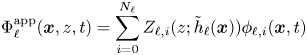
for $\ell =1,2$ , and $\{Z_{1,i}\}$
 and $\{Z_{2,i}\}$
 are appropriate function systems in the vertical coordinate $z$
 and may depend on $\tilde {h}_1(\boldsymbol {x})$
 and $\tilde {h}_2(\boldsymbol {x})$
 , respectively, which are the depths of the upper and the lower layers in the rest state, whereas $\boldsymbol {\phi }_\ell =(\phi _{\ell,0},\phi _{\ell,1},\ldots,\phi _{\ell,N_\ell })^\mathrm {T}$
 , $\ell =1,2$
 , are unknown variables. This yields a coupled system of equations for $\boldsymbol {\phi }_1$
 , $\boldsymbol {\phi }_2$
 and $\zeta$
 , depending on the function systems $\{Z_{1,i}\}$
 and $\{Z_{2,i}\}$
 , which we named Kakinuma model. Note that in our setting of the problem we have $\tilde {h}_1(\boldsymbol {x})=h_1$
 and $\tilde {h}_2(\boldsymbol {x})=h_2-b(\boldsymbol {x})$
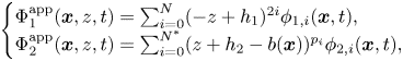
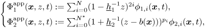
 . In this work, we study the Kakinuma model obtained when the approximate velocity potentials are defined by

where $N, N^*$ and $p_0,p_1,\ldots,p_{N^*}$
 are non-negative integers satisfying $0=p_0< p_1< \cdots < p_{N^*}$
 . Specifically, we show that the Kakinuma model obtained through the approximated potentials (1.2) with
(H1) $N^*=N$
 and $p_i=2i$ $(i=0,1,\ldots,N)$ in the case of the flat bottom $b(\boldsymbol {x})\equiv 0$,
(H2) $N^*=2N$
and $p_i=i$ $(i=0,1,\ldots,2N)$ in the case with general bottom topographies,


provides a higher order shallow water approximation to the full model for interfacial gravity waves in the strongly non-linear regime. The choice of the function systems as well as $N, N^*$ and $p_0,p_1,\ldots,p_{N^*}$
 is discussed and motivated later on.
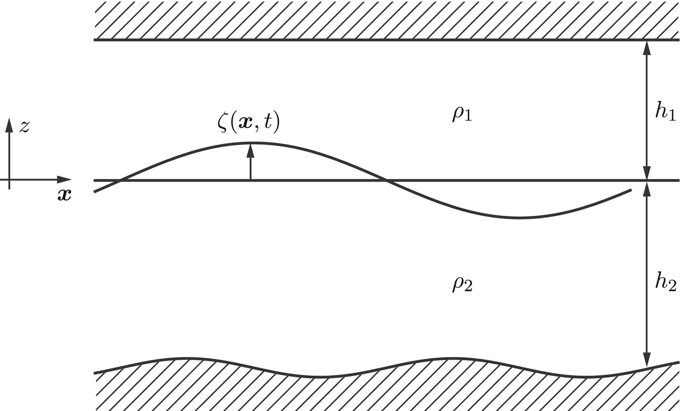
Figure 1. Internal gravity waves.
Comparison with surface gravity waves.
The Kakinuma model is an extension to interfacial gravity waves of the so-called Isobe–Kakinuma model for surface gravity waves, that is, water waves, in which Luke's Lagrangian density $\mathscr {L}_\mathrm {Luke}(\Phi,\zeta )$ , where $\zeta$
 is the surface elevation and $\Phi$
 is the velocity potential of the water, is approximated by a density $\mathscr {L}^\mathrm {app}(\boldsymbol {\phi },\zeta )=\mathscr {L}_\mathrm {Luke}(\Phi ^\mathrm {app},\zeta )$
 , where
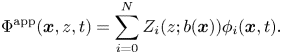
The Isobe–Kakinuma model was first proposed by Isobe [Reference Isobe21, Reference Isobe22] and then applied by Kakinuma to simulate numerically the water waves. Recently, this model was analysed from a mathematical point of view when the function system $\{Z_i\}$ is a set of polynomials in $z: Z_i(z;b(\boldsymbol {x}))=(z+h-b(\boldsymbol {x}))^{p_i}$
 with integers $p_i$
 satisfying $0=p_0< p_1<\cdots < p_N$
 . The initial value problem was analysed by Murakami and Iguchi [Reference Murakami and Iguchi35] in a special case and by Nemoto and Iguchi [Reference Nemoto and Iguchi36] in the general case. The hypersurface $t=0$
 in the space-time $\mathbf {R}^n\times \mathbf {R}$
 is characteristic for the Isobe–Kakinuma model in the sense that the operator acting on time derivatives of the unknowns has a non-trivial kernel. As a consequence, one needs to impose some compatibility conditions on the initial data for the existence of the solution. Under these compatibility conditions, the non-cavitation condition, and a Rayleigh–Taylor type condition $-\partial _z P^\mathrm {app} \geq c_0>0$
 on the water surface, where $P^\mathrm {app}$
 is an approximate pressure in the Isobe–Kakinuma model calculated from Bernoulli's equation, they showed the well-posedness of the initial value problem in Sobolev spaces locally in time. Moreover, Iguchi [Reference Iguchi18, Reference Iguchi19] showed that under the choice of the function system

the Isobe–Kakinuma model is a higher order shallow water approximation for the water wave problem in the strongly non-linear regime. Furthermore, Duchêne and Iguchi [Reference Duchêne and Iguchi13] showed that the Isobe–Kakinuma model also enjoys a Hamiltonian structure analogous to the one exhibited by Zakharov [Reference Zakharov43] on the full water wave problem and that the Hamiltonian of the Isobe–Kakinuma model is a higher order shallow water approximation to the one of the full water wave problem.
Our aim in the present paper and the companion paper [Reference Duchêne and Iguchi14] is to extend these results on surface gravity waves to the framework of interfacial gravity waves. With respect to surface gravity waves, our interfacial gravity waves framework brings two additional difficulties. The first one is that, due to the rigid-lid assumption, the full system for interfacial gravity waves described in § 2 features only one evolution equation for the two velocity potentials, and a constraint associated with the fixed fluid domain. From a physical perspective, the unknown velocity potential at the interface may be interpreted as a Lagrange multiplier associated with the constraint. A second important difference between water waves and interfacial gravity waves is that the latter suffer from Kelvin–Helmholtz instabilities. As a consequence, the initial value problem of the full model for interfacial gravity waves is ill-posed in Sobolev spaces; see Iguchi et al. [Reference Iguchi, Tanaka and Tani20], Kamotski and Lebeau [Reference Kamotski and Lebeau26]. This raises the question of the validity of any model for interfacial gravity waves. A partial answer is offered by the work of Lannes [Reference Lannes28], which proves the existence and uniqueness of solutions over large time intervals in the presence of interfacial tension. While interfacial tension effects are not expected to be the relevant regularization mechanism for the propagation of waves between, for instance, fresh and salted water, the key observation is that physical systems allow the propagation of waves with large amplitude and long wavelengths provided that some mechanism tames Kelvin–Helmholtz instabilities acting on the high-frequency component of the flow. This description is consistent with the fact that the initial value problem of the bi-layer shallow water system for the propagation of interfacial gravity waves in the hydrostatic framework is well-posed in Sobolev spaces under some hyperbolicity condition describing the absence of low-frequency Kelvin–Helmholtz instabilities, as proved by Bresch and Renardy [Reference Bresch and Renardy5]. Let us mention however that such a property is not automatic for higher order shallow water models. Specifically, we note that the Miyata–Choi–Camassa model derived by Miyata [Reference Miyata34] and Choi and Camassa [Reference Choi and Camassa8] and which can be regarded as a two-layer generalization of the Green–Naghdi equations for water waves turns out to overestimate Kelvin–Helmholtz estimates with respect to the full model; see Lannes and Ming [Reference Lannes and Ming30].
In [Reference Duchêne and Iguchi14], we analysed the initial value problem of the Kakinuma model when the approximated velocity potentials are defined by (1.2). We found that the Kakinuma model has a stability regime which can be expressed as

on the interface, where $H_1:= h_1 - \zeta$ and $H_2:=h_2 + \zeta - b$
 are the depths of the upper and the lower layers, $P_1^\mathrm {app}$
 and $P_2^\mathrm {app}$
 are approximate pressures of the fluids in the upper and the lower layers, $\alpha _1$
 and $\alpha _2$
 are positive constants depending only on $N$
 and on $p_0,p_1,\ldots,p_{N^*}$
 , respectively. This is a generalization of the aforementioned Rayleigh–Taylor type condition for the Isobe–Kakinuma model. It is worth noticing that, consistently with the expectation that the Kakinuma model is a higher order model for the full system for interfacial gravity waves and that the latter suffers from Kelvin–Helmholtz instabilities, the constants $\alpha _1$
 and $\alpha _2$
 converge to $0$
 as $N$
 and $N^*$
 go to infinity so that the stability condition becomes more and more stringent as $N$
 and $N^*$
 grow. When $N=N^*=0$
 , the Kakinuma model coincides with the aforementioned bi-layer shallow water system, and the stability regime coincides with the hyperbolic domain exhibited in [Reference Bresch and Renardy5]. Moreover, when the motion of the fluids together with the motion of the interface is in the rest state, the above stability condition is reduced to the well-known stable stratification condition

In [Reference Duchêne and Iguchi14], we showed that under the stability condition (1.5), the non-cavitation assumptions

and intrinsic compatibility conditions on the initial data, the initial value problem for the Kakinuma model is well-posed in Sobolev spaces locally in time. We also showed in [Reference Duchêne and Iguchi14] that the Kakinuma model enjoys a Hamiltonian structure analogous to the one exhibited by Benjamin and Bridges [Reference Benjamin and Bridges3] on the full model for interfacial gravity waves.
Comparison with other higher order models.
The Isobe–Kakinuma and the Kakinuma models belong to higher order models for the water waves and for the full interfacial gravity waves, respectively. By this we mean a family of systems of equations parametrized by nonnegative integers describing the order of the system within the family, that is $N$ for the Isobe–Kakinuma model, and whose solutions are expected to approach solutions to the full system as the order increases. Several such models have been introduced in the literature, mostly in the water waves framework, and we will restrict the discussion to water waves in this paragraph.
Based on a Taylor expansion of the Dirichlet-to-Neumann operator at stake in the water waves system with respect to the shape of the domain, Dommermuth and Yue [Reference Dommermuth and Yue10], West et al. [Reference West, Brueckner, Janda, Milder and Milton41] and Craig and Sulem [Reference Craig and Sulem9] have proposed the so-called high order spectral (HOS) models. While these models have been successfully employed in efficient numerical schemes (see recent accounts by Wilkening and Vasan [Reference Wilkening and Vasan42], Nicholls [Reference Nicholls37] and Guyenne [Reference Guyenne16]), the equations feature Fourier multipliers which prevent their direct use in situations involving non-trivial geometries such as horizontal boundaries. Moreover, the rigorous justification of HOS models is challenged by well-posedness issues; see the discussion in Ambrose et al. [Reference Ambrose, Bona and Nicholls1], and Duchêne and Melinand [Reference Duchêne and Melinand15].
A second class of higher order models originate from formal shallow water expansions put forward by Boussinesq [Reference Boussinesq4] and Rayleigh [Reference Rayleigh39]. A systematic derivation procedure has been described by Friedrichs in the appendix to [Reference Stoker40]. Recently, these higher order shallow water models have been described and discussed by Matsuno in [Reference Matsuno32, Reference Matsuno33] and Choi in [Reference Choi6, Reference Choi7]. The derivation procedure displays formula for approximate velocity potentials under form (1.3)–(1.4) (in particular, only even powers appear in the flat bottom case), with the important difference that the functions $\phi _{i}$ ($i=0,\ldots,N$
 ) are prescribed through explicit recursion relations. An important consequence of this derivation is that the resulting systems of equations involve only standard differential operators. However, the order of the differential operators at stake augments with the order of the system, which renders such models impractical for numerical simulations.
By contrast, the Isobe–Kakinuma model features only differential operators of order at most two acting on the variables $\phi _{i}$ ($i=0,\ldots,N$
 ) which are unknowns of the system. Notice that the size of the system augments with its order, $N$
 . However, the degrees of freedom do not augment with the order since, as mentioned above, some compatibility conditions must be satisfied. In fact all quantities are uniquely determined by two scalar functions which represent the canonical variables in the Hamiltonian formulation of the water waves system. Let us mention that function systems different from (1.4) have been considered by Athanassoulis and Belibassakis [Reference Athanassoulis and Belibassakis2], Klopman et al. [Reference Klopman, van Groesen and Dingemans27] and Papoutsellis and Athanassoulis [Reference Papoutsellis and Athanassoulis38] (see also references therein). While the systems obtained in these works have a similar nature, they are all different. We let the reader refer to Duchêne [Reference Duchêne11, chapter D] for an extended discussion and comparison of these models.
The choice of the function systems in (1.4) is motivated by the aforementioned Friedrichs expansion and is essential in the analysis of Iguchi [Reference Iguchi18, Reference Iguchi19] proving that the Isobe–Kakinuma model is a higher order shallow water approximation for the water wave problem in the strongly non-linear regime. We note that one may modify (1.4) by putting all odd and even terms $(z+h)^{i}$ for $i=0,1,\ldots$
 in the case of the flat bottom. However, in that case, one needs to use the terms up to order $2N$
 to keep the same precision of the approximation. Therefore, such a choice increases the number of unkonwns and equations by $N$
 so that it is undesirable for practical application. In other words, one can save memories in numerical simulations by using only even terms in the case of the flat bottom. On the contrary, if we put only odd terms $(z+h-b(\boldsymbol {x}))^{2i}$
 for $i=0,1,2,\ldots$
 in the case of a non-flat bottom, then the corresponding Isobe–Kakinuma model does not give any good approximation even if we take $N$
 a sufficiently large number, because the corresponding approximate velocity potential $\Phi ^\mathrm {app}$
 cannot approximate the boundary condition on the bottom so well due to the lack of odd order terms $(z+h-b(\boldsymbol {x}))^{2i+1}$
 for $i=0,1,2,\ldots$
 .
.
Following this discussion, the choice of the function systems (1.2) with (H1) or (H2) in our interfacial waves framework is very natural. In particular, the rigid-lid is assumed to be flat so that we do not need to use odd order terms $(-z+h_1)^{2i+1}$ for $i=0,1,2,\ldots$
 , in the approximate velocity potential $\Phi _1^\mathrm {app}$
 to obtain a good approximation, because $\Phi _1^\mathrm {app}$
 can approximate the boundary condition on the rigid-lid without such terms.
Description of the results.
In the present paper, we show that the Kakinuma model obtained through the approximated potentials (1.2) with
(H1) $N^*=N$
and $p_i=2i$ $(i=0,1,\ldots,N)$ in the case of the flat bottom $b(\boldsymbol {x})\equiv 0$,(H2) $N^*=2N$
and $p_i=i$ $(i=0,1,\ldots,2N)$ in the case with general bottom topographies,


provides a higher order shallow water approximation to the full model for interfacial gravity waves in the strongly non-linear regime. Our results apply to the dimensionless Kakinuma model obtained after suitable rescaling. The system of equations then depend on the positive dimensionless parameters $\delta _1$ and $\delta _2$
 which are shallowness parameters related to the upper and the lower layers, respectively, that is, $\delta _\ell =\frac {h_\ell }{\lambda }$ $(\ell =1,2)$
 with the typical horizontal wavelength $\lambda$
 . The shallow water regime is described through the smallness of the parameters $\delta _1$
 and $\delta _2$
 . What is more, our results are uniform with respect to parameters satisfying either $\rho _2\lesssim \rho _1<\rho _2$
 , or $\rho _1\ll \rho _2$
 and $h_2\lesssim h_1$
 . We notice that the rigid-lid framework is expected to be invalid in the regime $\rho _1\ll \rho _2$
 and $h_1\ll h_2$
 which is excluded in this paper; see Duchêne [Reference Duchêne12].
Our first result extends the result of [Reference Duchêne and Iguchi14] on the well-posedness of the initial value problem by showing that solutions to the dimensionless Kakinuma model are defined on a time interval which does not vanish for arbitrarily small values of $\delta _1$ and $\delta _2$
 .
.
Theorem 1.1 Long-time well-posedness
Under the (dimensionless) stability condition (1.5), the (dimensionless) non-cavitation assumptions (1.7) and intrinsic compatibility conditions on the initial data, the initial value problem for the Kakinuma model is well-posed in Sobolev spaces on a time interval which is independent of $\delta _1\in (0,1]$ and $\delta _2\in (0,1]$
 .
.
While the non-cavitation assumption and the stability condition are automatically satisfied for small initial data and small bottom topography $b$ , an arrangement of non-trivial initial data satisfying the compatibility conditions with suitable bounds is a non-trivial issue, and demands a specific analysis.
Proposition 1.2 Initial data satisfying the compatibility conditions and necessary bounds in theorem 1.1 are uniquely determined (up to an additive constant) by sufficiently regular initial data for the canonical variables of the Hamiltonian structure.
Then, we show that under the special choice of the indices $p_0,p_1,\ldots,p_{N^*}$ as in (H1) or (H2), the dimensionless Kakinuma model is consistent with the full model for interfacial gravity waves with an error of order $O(\delta _1^{4N+2}+\delta _2^{4N+2})$
 .
.
Theorem 1.3 Consistency
Assume (H1) or (H2). The solutions to the dimensionless Kakinuma model constructed in theorem 1.1 produce functions that satisfy approximately the dimensionless full interfacial gravity waves system up to error terms of size $O(\delta _1^{4N+2}+\delta _2^{4N+2})$ .
.
Conversely, solutions to the dimensionless full interfacial gravity waves system satisfying suitable uniform bounds produce through proposition 1.2 functions that satisfy approximately the dimensionless Kakinuma model up to error terms of size $O(\delta _1^{4N+2}+\delta _2^{4N+2})$ .
.
In the last result, we assume the existence of a solution to the full model with a uniform bound since for general initial data in Sobolev spaces, one cannot expect to construct a solution to the initial value problem, due to the ill-posedness of the problem discussed previously. The same issue arises for the full justification of the Kakinuma model.
Theorem 1.4 Full justification
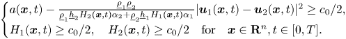
Assuming the existence of a solution to the dimensionless full interfacial gravity waves system with a uniform bound and satisfying initially the (dimensionless) stability condition (1.5) and (dimensionless) non-cavitation assumptions (1.7), then the Kakinuma model with (H1) or (H2) and appropriate initial data produces an approximate solution with the error estimate

on some time interval independent of $\delta _1\in (0,1]$ and $\delta _2\in (0,1]$
 , where $\zeta ^{{\rm K}}$
 and $\zeta ^{{\rm IW}}$
 are solutions to the dimensionless Kakinuma model and to the full model, respectively.
In our last main result, we show that the Hamiltonian structure of the Kakinuma model is a shallow water approximation of the Hamiltonian structure of the full interfacial gravity waves model.
Theorem 1.5 Hamiltonians
Assume (H1) or (H2). Under appropriate assumptions on the canonical variables $(\zeta,\phi )$ , we have

where $\mathscr {H}^{{\rm K}}$ and $\mathscr {H}^{{\rm IW}}$
 are the Hamiltonians of the dimensionless Kakinuma model and of the dimensionless full interfacial gravity waves model, respectively.
Remark 1.6 The precise statements of our main results are displayed in § 3. Specifically, theorem 1.1 corresponds to theorem 3.1, proposition 1.2 corresponds to proposition 3.4, theorem 1.3 corresponds to theorems 3.5 and 3.6 (see also remark 3.8), theorem 1.4 corresponds to theorem 3.9, and theorem 1.5 corresponds to theorem 3.10.
Structures of the Kakinuma model.
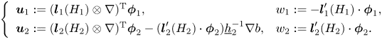
In order to obtain our main results, we exploit several structures of the Kakinuma model. The Kakinuma model can be written compactly as

where we denote ${\boldsymbol \phi }_1 := (\phi _{1,0},\phi _{1,1},\ldots,\phi _{1,N})^\mathrm {T}$ , ${\boldsymbol \phi }_2 := (\phi _{2,0},\phi _{2,1},\ldots,\phi _{2,N^*})^\mathrm {T}$
 , put ${\boldsymbol l}_1(H_1) := (1,H_1^2,H_1^4,\ldots,H_1^{2N})^\mathrm {T}$
 , ${\boldsymbol l}_2(H_2) := (1,H_2^{p_1},H_2^{p_2},\ldots,H_2^{p_{N^*}})^\mathrm {T}$
 , and the linear operators $L_\ell$
 , and functions ${\boldsymbol u}_\ell$
 and $w_\ell$
 for $\ell =1,2$
 are defined (after non-dimensionalization) in § 3. Here we recognize the fact that the hypersurface $t=0$
 in the space-time $\mathbf {R}^n\times \mathbf {R}$
 is characteristic for the Kakinuma model, since the system of evolution equations is overdetermined for the variable $\zeta$
 , and underdetermined for the variables ${\boldsymbol \phi }_1$
 and ${\boldsymbol \phi }_2$
 . As a consequence, solutions to the Kakinuma model must satisfy some compatibility conditions. Introducing linear operators $\mathcal {L}_{1,i}$ $(i=0,\ldots,N)$
 acting on ${\boldsymbol \varphi }_1 = (\varphi _{1,0},\ldots,\varphi _{1,N})^\mathrm {T}$
 and $\mathcal {L}_{2,i}$ $(i=0,\ldots,N^*)$
 acting on ${\boldsymbol \varphi }_2 = (\varphi _{2,0},\ldots,\varphi _{2,N^*})^\mathrm {T}$
 by
by

the necessary conditions can be written simply as
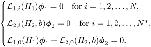
The first two vectorial identities are analogous to the compatibility conditions of the Isobe–Kakinuma model for water waves, while the last identity is specific to the bi-layer framework and is related to the continuity of the normal component of the velocity at the interface.
A first key ingredient of the analysis is the fact that for sufficiently regular functions $\zeta$ , $b$
, $b$ and $\phi _1$
 (respectively $\phi _2$
 ), there exists a unique solution ${\boldsymbol \phi }_1$
 (respectively ${\boldsymbol \phi }_2$
 ) to the problems

satisfying suitable elliptic estimates. What is more, the well-defined linear operators
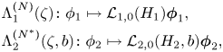
are found to approximate the corresponding Dirichlet-to-Neumann maps $\Lambda _1(\zeta )$ and $\Lambda _2(\zeta,b)$
 defined by

where $\Phi _1$ and $\Phi _2$
 are the unique solutions to Laplace's equations

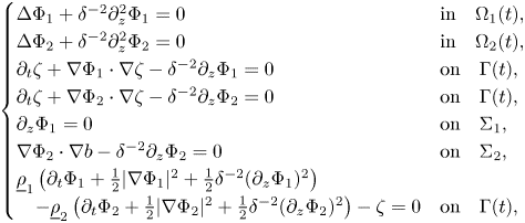
where we denote the upper layer, the lower layer, the interface, the rigid-lid and the bottom at time $t$ by $\Omega _1(t)$
 , $\Omega _2(t)$
 , $\Gamma (t)$
 , $\Sigma _1$
 and $\Sigma _2$
 , respectively. Specifically, it is proved that, under the special choice of the indices $p_0,p_1,\ldots,p_{N^*}$
 in (H1) or (H2) and after suitable rescaling, the difference between the dimensionless operators is of size $O(\delta _1^{4N+2}+\delta _2^{4N+2})$
 . This analysis, which follows directly from the corresponding analysis for surface waves developed in [Reference Iguchi19] and scaling arguments, provides the key argument in the proof of the consistency result described in theorem 1.3.
In order to study the Kakinuma model, we also need to analyse the full elliptic system
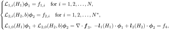
for sufficiently regular functions $\zeta$ , $b$
, $b$ and ${\boldsymbol f}_1=(f_{1,1},\ldots f_{1,N})^\mathrm {T},{\boldsymbol f}_2=(f_{2,1},\ldots, f_{2,N^*})^\mathrm {T},{\boldsymbol f}_3,f_4$
 . The ellipticity of the problem relies on the coercivity of the corresponding operators $L_1(H_1)$
 and $L_2(H_2)$
 . The solvability of (1.11) is essential in several directions. Firstly, it provides an alternative consistency result, where solutions to the full interfacial gravity waves system produce approximate solutions to the Kakinuma model but satisfying exactly and not approximately the necessary conditions (1.9). In turn, this provides a crucial ingredient to the full justification of the Kakinuma model described in theorem 1.4. Furthermore, the arrangement of initial data satisfying the compatibility conditions as stated in proposition 1.2 amounts to solving (1.11) with ${\boldsymbol f}_1={\boldsymbol 0}$
 , ${\boldsymbol f}_2={\boldsymbol 0}$
 , ${\boldsymbol f}_3={\boldsymbol 0}$
 and $f_4=\phi$
 . Similarly, our result on the Hamiltonians $\mathscr {H}^{\text {K}}$
 and $\mathscr {H}^{\text {IW}}$
 described in theorem 1.5 relies on a comparison of solutions to (1.11) with ${\boldsymbol f}_1={\boldsymbol 0}$
 , ${\boldsymbol f}_2={\boldsymbol 0}$
 , ${\boldsymbol f}_3={\boldsymbol 0}$
 and $f_4=\phi$
 and solutions to

thus extending to the interfacial gravity waves framework the analysis in [Reference Duchêne and Iguchi13]. Finally, the solvability of (1.11) allows to determine and control time derivatives $\partial _t{\boldsymbol \phi }_1$ and $\partial _t{\boldsymbol \phi }_2$
 of sufficiently regular solutions to the Kakinuma model (1.8) by using the equations obtained when differentiating with respect to time the compatibility conditions (1.9) combined with the last equation of (1.8). This is a crucial ingredient for the analysis of the initial value problem.
Another crucial ingredient for the analysis of the initial value problem concerns uniform energy estimates on the linearized Kakinuma system. To this end, we write the linearized system under the form

where $\dot {\boldsymbol {U}}:=(\dot {\zeta }, \dot {\boldsymbol {\phi }}_1, \dot {\boldsymbol {\phi }}_2)^\mathrm {T}$ is the deviation from the reference state $\boldsymbol {U}:=({\zeta }, {\boldsymbol {\phi }}_1, {\boldsymbol {\phi }}_2)^\mathrm {T}$
 , $\boldsymbol {u}$
 is a suitable velocity which is a convex combination of $\boldsymbol {u}_1$
 and $\boldsymbol {u}_2$
 whose weights depend on $\rho _\ell$
 , $H_\ell$
 as well as $\alpha _\ell$
 ($\ell =1,2$
 ) the positive constants mentioned previously, $\dot {\boldsymbol {F}}$
 represents lower order terms and $\mathscr {A}_1:=\mathscr {A}_1(\boldsymbol {U})$
 is a skew-symmetric matrix and $\mathscr {A}_0^\mathrm {mod}:=\mathscr {A}_0^\mathrm {mod}(\boldsymbol {U})$
 is a linear operator symmetric in $L^2$
 . The energy function associated to (1.12) is given by $(\mathscr {A}_0^\mathrm {mod}\dot {\boldsymbol {U}},\dot {\boldsymbol {U}})_{L^2}$
 , and we prove that

under the non-cavitation assumption (1.7) and the stability condition (1.5). Because the structure of (1.12) is not standard, the control of the energy function is obtained by testing (1.12) with the time derivatives, $\partial _t\dot {\boldsymbol {U}}$ . This, together with suitable product and commutator estimates in Sobolev spaces, provides the a priori control of the energy function for solutions to the Kakinuma model and their derivatives, and we show that this control is uniform in the shallow water regime after suitable rescaling. Since the construction and uniqueness of a solution was obtained in the companion paper [Reference Duchêne and Iguchi14], the uniform estimates provide the proof of the long-time well-posedness of the initial value problem for the Kakinuma model result stated in theorem 1.1. Furthermore, using the aforementioned consistency result, we prove that the difference between solutions to the full interfacial gravity waves system and corresponding solutions to the Kakinuma model satisfy an identity analogous to (1.12), and hence infer a control of the energy function of the difference and its derivatives, which yields the full justification of the Kakinuma model stated in theorem 1.4.
Outline.
The contents of this paper are as follows. In § 2 we first recall the basic equations governing the interfacial gravity waves and write down the Kakinuma model that we are going to analyse in this paper, and then rewrite them in a non-dimensional form by introducing several non-dimensional parameters. Hamiltonians of the full model and of the Kakinuma model in the non-dimensional variables are also provided. In § 3 we first introduce some differential operators, which enable us to write the Kakinuma model simply in form (1.8), and then we present the precise statements of our main results in this paper. In § 4 we first recall results in the framework of surface waves related to the consistency of the Isobe–Kakinuma model, and then prove theorems 3.5 and 3.6 concerning the consistency of the Kakinuma model by a simple scaling argument. In § 5 we first derive an elliptic estimate related to the compatibility conditions for the Kakinuma model, which explains how to prepare the initial data, as stated in proposition 3.4. Then we give uniform a priori bounds on regular solutions to the Kakinuma model, especially, a priori bounds of time derivatives. In § 6 we provide uniform energy estimates for the solution to the Kakinuma model and prove theorem 3.1, which ensures the existence of the solution to the initial value problem for the Kakinuma model on a time interval independent of parameters, especially, $\delta _1$ and $\delta _2$
 , under the stability condition, the non-cavitation assumptions and intrinsic compatibility conditions on the initial data, together with a uniform bound of the solution. In § 7 we first give a supplementary estimate on an approximation of the Dirichlet-to-Neumann map, and then revisit the consistency of the Kakinuma model. We prove proposition 7.6, which is another version of the consistency given in theorem 3.6, where we adopt a different construction of an approximate solution to the Kakinuma model from the solution to the full model. Then, by making use of the well-posedness of the initial value problem for the Kakinuma model, we prove theorem 3.9 which provides a conditional rigorous justification of the Kakinuma model, that is, assuming the existence of a solution to the full model with a uniform bound, we derive an error estimate between a corresponding solution to the Kakinuma model and that of the full model. Finally, in § 8 we prove theorem 3.10 which gives an error estimate between the Hamiltonian of the Kakinuma model and that of the full model. For the convenience of the reader, the structure of the paper and proofs dependencies are sketched in figure 2.
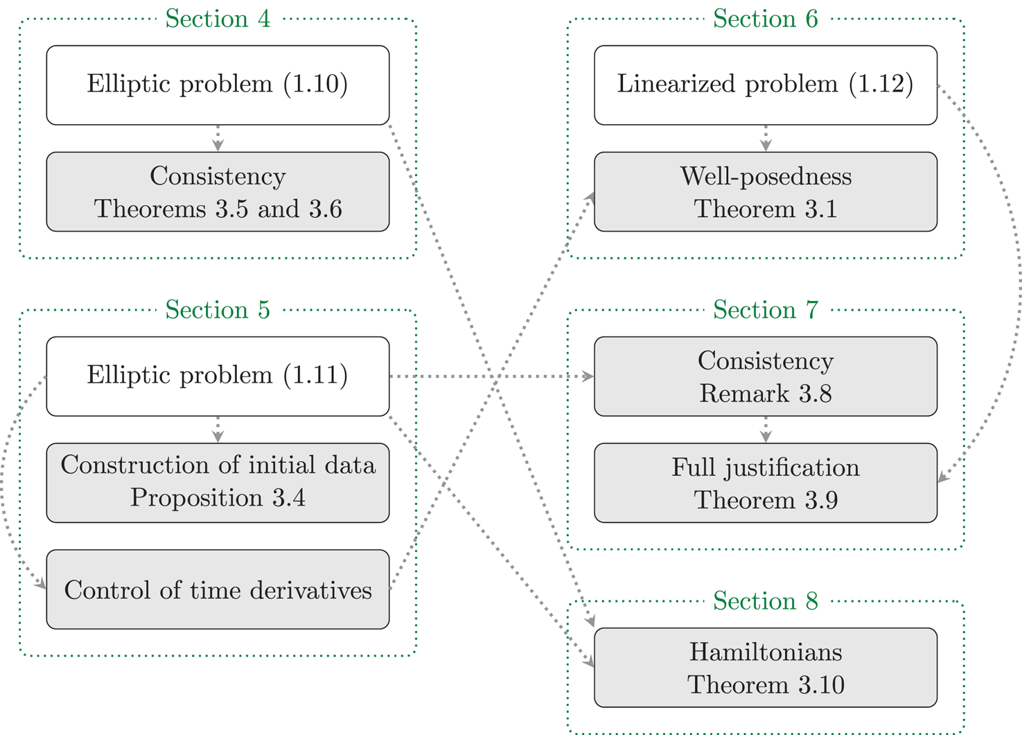
Figure 2. Articulation of the proofs.
Notation.
We denote by $W^{m,p}$ the $L^p$
 Sobolev space of order $m$
 on $\mathbf {R}^n$
 and $H^m=W^{m,2}$
 . We put $\mathring {H}^m=\{ \phi \,;\, \nabla \phi \in H^{m-1}\}$
 . The norm of a Banach space $B$
 is denoted by $\|\cdot \|_B$
 . The $L^2$
 -inner product is denoted by $(\cdot,\cdot )_{L^2}$
 . We put $\partial _t=\frac {\partial }{\partial t}$
 , $\partial _j=\partial _{x_j}=\frac {\partial }{\partial x_j}$
 and $\partial _z=\frac {\partial }{\partial z}$
 . $[P,Q]=PQ-QP$
 denotes the commutator and $[P;u,v]=P(uv)-(Pu)v-u(Pv)$
 denotes the symmetric commutator. For a matrix $A$
 we denote by $A^\mathrm {T}$
 the transpose of $A$
 . $O$
. $O$ denotes a zero matrix. For a vector $\boldsymbol{\phi}=(\phi _0,\phi _1,\ldots,\phi _N)^\mathrm {T}$
 we denote the last $N$
 components by $\boldsymbol{\phi'}=(\phi _1,\ldots,\phi _N)^\mathrm {T}$
 . $f \lesssim g$
 means that there exists a non-essential positive constant $C$
 such that $f \leq Cg$
 holds. $f \simeq g$
 means that $f \lesssim g$
 and $g \lesssim f$
 hold.
hold.
2. The basic equations and the Kakinuma model
2.1. Equations with physical variables
We first recall the equations governing potential flows for two layers of immiscible, incompressible, homogeneous and inviscid fluids, and then write down the Kakinuma model at stake in this work. In the following, we denote the upper layer, the lower layer, the interface, the rigid-lid and the bottom at time t by $\Omega _1(t)$ , $\Omega _2(t)$
 , $\Gamma (t)$
 , $\Sigma _1$
 and $\Sigma _2$
 , respectively. The velocity potentials $\Phi _1(\boldsymbol {x},z,t)$
 and $\Phi _2(\boldsymbol {x},z,t)$
 in the upper and lower layers, respectively, satisfy Laplace's equations

where $\Delta =\partial _1^2+\cdots +\partial _n^2$ is the Laplacian with respect to the horizontal space variables $\boldsymbol {x}=(x_1,\ldots,x_n)$
 . Bernoulli's laws of each layers have the form


where $\nabla =(\partial _1,\ldots,\partial _n)$ , the positive constant $g$
 is the acceleration due to gravity, and $P_1(\boldsymbol {x},z,t)$
 and $P_2(\boldsymbol {x},z,t)$
 are pressures in the upper and lower layers, respectively. The dynamical boundary condition on the interface is given by

The kinematic boundary conditions on the interface, the rigid-lid and the bottom are given by


These are the basic equations for interfacial gravity waves. It follows from Bernoulli's laws (2.3)–(2.4) and the dynamical boundary condition (2.5) that

We will always assume the stable stratification condition $(\rho _2-\rho _1)g > 0$ . As in the case of surface water waves, the basic equations have a variational structure and the corresponding Luke's Lagrangian is given, up to terms which do not contribute to the variation of the Lagrangian, by the vertical integral of the pressure in the water regions. After using Bernoulli's laws (2.3)–(2.4) we can find the Lagrangian density
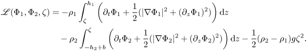
In fact, one checks readily that (2.1)–(2.2) and (2.6)–(2.10) are Euler–Lagrange equations associated with the action function

We proceed to the Kakinuma model. Let $N$ and $N^*$
 be non-negative integers. In view of the analysis for the Isobe–Kakinuma model for surface water waves, we approximate the velocity potentials $\Phi _1$
 and $\Phi _2$
 in the Lagrangian by
where $p_0,p_1,\ldots,p_{N^*}$ are non-negative integers satisfying $0=p_0< p_1<\cdots < p_{N^*}$
 . Plugging (2.12) into the Lagrangian density (2.11), we obtain an approximate Lagrangian density

where $\boldsymbol {\phi }_1:=(\phi _{1,0},\phi _{1,1},\ldots,\phi _{1,N})^\mathrm {T}$ and $\boldsymbol {\phi }_2:=(\phi _{2,0},\phi _{2,1},\ldots,\phi _{2,N^*})^\mathrm {T}$
 . The corresponding Euler–Lagrange equation is the Kakinuma model, which has the form

where $H_1$ and $H_2$
 are depths of the upper and the lower layers, that is,

In (2.13), we used the notational convention $0/0 = 0$ . More precisely, this convention was used so as to dictate $p_0/(p_0+p_0)=0$
 and $p_0p_1/(p_0+p_1-1)=0$
 in the case $p_1=1$
 . We recall also that $p_0=0$
 is always assumed.
2.2. The dimensionless equations
In order to rigorously validate the Kakinuma model (2.13) as a higher order shallow water approximation of the full model for interfacial gravity waves (2.1)–(2.9), we first introduce non-dimensional parameters and then non-dimensionalize the equations, through a convenient rescaling of variables. Let $\lambda$ be a typical horizontal wavelength. Following Lannes [Reference Lannes28], we introduce a non-dimensional parameter $\delta$
 by
by

where $\underline {\rho }_1$ and $\underline {\rho }_2$
 are relative densities. We also need to use relative depths $\underline {h}_1$
 and $\underline {h}_2$
 of the layers. These non-dimensional parameters are defined by

which satisfy the relations

Note also that $\min \{h_1,h_2\} \leq h \leq \max \{h_1,h_2\}$ . It follows from the second relation in (2.14) that

Here, we note that the standard shallowness parameters $\delta _1:=\frac {h_1}{\lambda }$ and $\delta _2:=\frac {h_2}{\lambda }$
 relative to the upper and the lower layers, respectively, are related to the above parameters by $\delta _\ell = \underline {h}_\ell \delta$
 for $\ell =1,2$
 . In many results of this paper, we restrict our consideration to the parameter regime

To understand this restriction, it is convenient to use non-dimensional parameters $\gamma :=\frac {\rho _1}{\rho _2}$ and $\theta :=\frac {h_1}{h_2}$
 . In terms of these parameters, $\underline {h}_\ell ^{-1}$ $(\ell =1,2)$
 can be represented as

Therefore, the only cases that (2.16) excludes are the case $\gamma,\theta \ll 1$ and the case $\gamma,\theta \gg 1$
 . Since we shall also assume the stable stratification condition $(\rho _2-\rho _1)g>0$
 , we can describe the two regimes considered in this paper as
(i) $\gamma \simeq 1$
, i.e. $\rho _1\simeq \rho _2$,(ii) $\gamma \ll 1$
and $\theta \gtrsim 1$, i.e. $\rho _1\ll \rho _2$ and $h_2\lesssim h_1$.


Introducing $c_{\text SW} :=\sqrt { (\underline {\rho }_2-\underline {\rho }_1)gh }$ the speed of infinitely long and small interfacial gravity waves, we rescale the independent and the dependent variables by

Plugging these into the full model (2.1)–(2.2) and (2.6)–(2.10) and dropping the tilde sign in the notation we obtain
where in this scaling the upper layer $\Omega _1(t)$ , the lower layer $\Omega _2(t)$
 , the interface $\Gamma (t)$
 , the rigid-lid $\Sigma _1$
 and the bottom $\Sigma _2$
 are written as

Denoting

and using the chain rule, the above system can be written in a more compact and closed form as

where $\Lambda _1(\zeta,\delta,\underline {h}_1)$ and $\Lambda _2(\zeta,b,\delta,\underline {h}_2)$
 are the Dirichlet-to-Neumann maps for Laplace's equations. More precisely, these are defined by

where $\Phi _1$ and $\Phi _2$
 are unique solutions to the boundary value problems

As for the Kakinuma model, we introduce additionally the rescaled variables

where we recall that $p_0,p_1,\ldots,p_{N^*}$ are non-negative integers satisfying ${0=p_0< p_1<\cdots < p_{N^*}}$
 appearing in the approximation (2.12). Plugging these and the previous scaling into the Kakinuma model (2.13) and dropping the tilde sign in the notation we obtain the Kakinuma model in the non-dimensional form, which is written as

where we used the notational convention $0/0 = 0$ , and
, and

We impose the initial conditions to the Kakinuma model of the form

2.3 Hamiltonian structures
Benjamin and Bridges [Reference Benjamin and Bridges3] found that the full model for interfacial gravity waves can be written in Hamilton's canonical form

where the canonical variable $\phi$ is defined by

and the Hamiltonian $\mathscr {H}^{{\rm IW}}$ is the total energy $\mathscr {E}$
 written in terms of the canonical variables $(\zeta,\phi )$
 . Specifically, $\mathscr {E}$
 is the sum of the kinetic energies of the fluids in the upper and the lower layers and the potential energy due to the gravity defined as

Here and in what follows, we denote simply $\Lambda _1(\zeta )=\Lambda _1(\zeta,\delta,\underline {h}_1)$ and $\Lambda _2(\zeta )=\Lambda _2(\zeta,b,\delta,\underline {h}_2)$
 . It follows from the kinematic boundary conditions on the interface that $\Lambda _1(\zeta )\phi _1+\Lambda _2(\zeta )\phi _2=0$
 , so that $\phi _1$
 and $\phi _2$
 can be written in terms of the canonical variables $(\zeta,\phi )$
 as
as

Therefore, the Hamiltonian $\mathscr {H}^{{\rm IW}}(\zeta,\phi )$ of the full model for interfacial gravity waves is given explicitly by

As was shown in the companion paper [Reference Duchêne and Iguchi14], the Kakinuma model (2.18) also enjoys a Hamiltonian structure analogous to that of the full model for interfacial gravity waves. The canonical variables are the elevation of the interface $\zeta$ and $\phi$
 defined by

where $\Phi _\ell ^\mathrm {app}$ $(\ell =1,2)$
 are non-dimensional versions of the approximate velocity potentials, which are defined by
and $H_\ell$ $(\ell =1,2)$
 are depths of the upper and lower layers defined by (2.19). We note that if the canonical variables $(\zeta,\phi )$
 are given, then the Kakinuma model (2.18) determines $\boldsymbol {\phi }_1=(\phi _{1,0},\phi _{1,1},\ldots,\phi _{1,N})^\mathrm {T}$
 and $\boldsymbol {\phi }_2=(\phi _{2,0},\phi _{2,1},\ldots,\phi _{2,N^*})^\mathrm {T}$
 , which are unique up to an additive constant of the form $(\mathcal {C}\underline {\rho }_1,\mathcal {C}\underline {\rho }_2)$
 to $(\phi _{1,0},\phi _{2,0})$
 . For details, we refer to [Reference Duchêne and Iguchi14, § 8.1] and lemma 5.1 in § 5. Then, the Hamiltonian $\mathscr {H}^{{\rm K}}(\zeta,\phi )$
 of the Kakinuma model is given by

3. Statements of the main results
Before stating the main results in this paper, let us introduce some notations which allow in particular to rewrite (2.18) in a compact form. We introduce second order differential operators $L_{1,ij} = L_{1,ij}(H_1,\delta,\underline {h}_1)$ $(i,j=0,1,\ldots,N)$
 and $L_{2,ij} = L_{2,ij}(H_2,b,\delta,\underline {h}_2)$ $(i,j=0,1,\ldots,N^*)$
 by
by


where we use the notational convention $0/0 = 0$ . Notice that we have $(L_{\ell,ij})^*=L_{\ell,ji}$
 for $\ell =1,2$
 , where $(L_{\ell,ij})^*$
 is the adjoint operator of $L_{\ell,ij}$
 in $L^2(\mathbf {R}^n)$
 . We put ${\boldsymbol \phi }_1 := (\phi _{1,0},\phi _{1,1},\ldots,\phi _{1,N})^\mathrm {T}$
 , ${\boldsymbol \phi }_2 := (\phi _{2,0},\phi _{2,1},\ldots,\phi _{2,N^*})^\mathrm {T}$
 and
and

and define ${\boldsymbol u}_\ell$ and $w_\ell$
 for $\ell =1,2$
 , which represent approximately the horizontal and the vertical components of the velocity field on the interface from the water region $\Omega _\ell (t)$
 , by
, by
Then, denoting $L_1 := (L_{1,ij})_{0\leq i,j\leq N}$ and $L_2 := (L_{2,ij})_{0\leq i,j\leq N^*}$
 we can write the Kakinuma model (2.18) more compactly as

By eliminating $\partial _t\zeta$ from the first two vectorial identities in (3.5), we obtain $N+N^*+1$
 scalar relations which are necessary conditions for the existence of solutions to the Kakinuma model, as stated below. Introducing linear operators $\mathcal {L}_{1,i} := \mathcal {L}_{1,i}(H_1,\delta,\underline {h}_1)$ $(i=0,\ldots,N)$
 acting on ${\boldsymbol \varphi }_1 = (\varphi _{1,0},\ldots,\varphi _{1,N})^\mathrm {T}$
 and $\mathcal {L}_{2,i} := \mathcal {L}_{2,i}(H_2,b,\delta,\underline {h}_2)$ $(i=0,\ldots,N^*)$
 acting on ${\boldsymbol \varphi }_2 = (\varphi _{2,0},\ldots,\varphi _{2,N^*})^\mathrm {T}$
 by
by

the necessary conditions can be written simply as

Hereafter, these necessary conditions will be referred to as the compatibility conditions. Notice that under these compatibility conditions we have for $\ell =1,2$
where $\boldsymbol {l}_\ell =\boldsymbol {l}_\ell (H_\ell )$ and similar simplifications of notations will be used in the following without any comments. In connection with the stability condition (1.5), we introduce a function

which corresponds to $- (\partial _z (P_2^\mathrm {app} - P_1^\mathrm {app} ))|_{\Gamma (t)}$ in the stability condition.
Our first main result in this paper is the existence of the solution to the initial value problem (2.18)–(2.20) for the Kakinuma model on a time interval independent of parameters, especially, the shallowness parameters $\delta _1=\underline {h}_1\delta$ and $\delta _2=\underline {h}_2\delta$
 together with a uniform bound of the solution. For simplicity, we denote $H_{\ell (0)}:=H_\ell |_{t=0}$
 , $\boldsymbol {u}_{\ell (0)}:=\boldsymbol {u}_\ell |_{t=0}$
 for $\ell =1,2$
 and $a_{(0)}:=a|_{t=0}$
 , which can be written in terms of the initial data according to the initial condition (2.20). Although the function $a$
 includes the terms $(\partial _t\boldsymbol {\phi }_\ell ')|_{t=0}$
 for $\ell =1,2$
 , where $\boldsymbol {\phi }_1'=(\phi _{1,1},\ldots,\phi _{1,N})^\mathrm {T}$
 and $\boldsymbol {\phi }_2'=(\phi _{2,1},\ldots,\phi _{2,N^*})^\mathrm {T}$
 , and the hypersurface $t=0$
 is characteristic for the Kakinuma model, we can uniquely determine them in terms of the initial data. For details, we refer to remark 5.3.
Theorem 3.1 Let $c_0, M_0, \underline {h}_\mathrm {min}$ be positive constants and $m$
 an integer such that ${m>\frac {n}{2}+1}$
 . There exist a time $T>0$
 and a constant $M>0$
 such that for any positive parameters $\underline {\rho }_1, \underline {\rho }_2, \underline {h}_1, \underline {h}_2, \delta$
 satisfying the natural restrictions (2.14), ${\underline {h}_1\delta, \underline {h}_2\delta \leq 1}$
 , as well as the condition ${\underline {h}_\mathrm {min} \leq \underline {h}_1, \underline {h}_2}$
 , if the initial data $(\zeta _{(0)},\boldsymbol {\phi }_{1(0)},\boldsymbol {\phi }_{2(0)})$
 and the bottom topography $b$
 satisfy

the non-cavitation assumption

the stability condition

with positive constants $\alpha _1$ and $\alpha _2$
 defined by (3.16), and the compatibility conditions

then the initial value problem (2.18)–(2.20) has a unique solution $(\zeta,\boldsymbol {\phi }_1,\boldsymbol {\phi }_2)$ on the time interval $[0,T]$
 satisfying
where we recall the notation ${\boldsymbol \phi }_1^{\prime } = (\phi _{1,1},\phi _{1,2},\ldots,\phi _{1,N})^\mathrm {T}$ and ${\boldsymbol \phi }_2^{\prime } = (\phi _{2,1},\phi _{2,2},\ldots, \phi _{2,N^*})^\mathrm {T}$
 . Moreover, the solution satisfies the uniform bound

for $t\in [0,T]$ together with
Remark 3.2 The constants $\alpha _1$ and $\alpha _2$
 are defined by
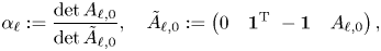
for $\ell =1,2$ , where $\boldsymbol {1}:=(1,\ldots,1)^\mathrm {T}$
 and the matrices $A_{1,0}$
 and $A_{2,0}$
 are defined by

Hence, $\alpha _1$ and $\alpha _2$
 are positive constants depending only on $N$
 and the non-negative integers $0=p_0< p_1<\ldots < p_{N^*}$
 , respectively, and go to $0$
 as $N,N^*\to \infty$
 .
.
Remark 3.3 It is easy to check that the non-cavitation assumption (3.11) and the stability condition (3.12) are automatically satisfied for small initial data $(\zeta _{(0)},\boldsymbol {\phi }_{1(0)},\boldsymbol {\phi }_{2(0)})$ and small bottom topography $b$
 , whereas an arrangement of non-trivial initial data satisfying the compatibility conditions (3.13) together with the uniform bound (3.10) is a non-trivial issue. To this end, we use the canonical variable $\phi$
 defined by (2.23), which can be written as

Given the initial data $(\zeta _{(0)},\phi _{(0)})$ for the canonical variables $(\zeta,\phi )$
 , and the bottom topography $b$
 , the necessary conditions (3.7) and the above relation (3.17) determine the initial data $(\boldsymbol {\phi }_{1(0)},\boldsymbol {\phi }_{2(0)})$
 for the Kakinuma model (2.18)–(2.20) satisfying the compatibility conditions (3.13) and the uniform bound (3.10), which is unique up to an additive constant of the form $(\mathcal {C}\underline {\rho }_2,\mathcal {C}\underline {\rho }_1)$
 to $(\phi _{1,0(0)},\phi _{2,0(0)})$
 . In fact, we have the following proposition, which is a simple corollary of lemma 5.1 given in § 5.
Proposition 3.4 Let $c_0, M_0$ be positive constants and $m$
 an integer such that $m>\frac {n}{2}+1$
 . There exists a positive constant $C$
 such that for any positive parameters $\underline {\rho }_1, \underline {\rho }_2, \underline {h}_1, \underline {h}_2, \delta$
 satisfying the natural restrictions (2.14) and $\underline {h}_1\delta, \underline {h}_2\delta \leq 1$
 , if the initial data $(\zeta _{(0)},\phi _{(0)})\in H^m\times \mathring {H}^m$
 of the canonical variables, the bottom topography $b\in W^{m,\infty }$
 , and initial depths $H_{1(0)} := 1 - \underline {h}_1^{-1}\zeta _{(0)}$
 and $H_{2(0)} := 1 + \underline {h}_2^{-1}\zeta _{(0)} - \underline {h}_2^{-1}b$
 satisfy

then there exist initial data $(\boldsymbol {\phi }_{1(0)},\boldsymbol {\phi }_{2(0)})$ satisfying the compatibility conditions (3.13) as well as $\phi _{(0)} = \underline {\rho }_2\boldsymbol {l}_2(H_{2(0)})\cdot \boldsymbol {\phi }_{2(0)} - \underline {\rho }_1\boldsymbol {l}_1(H_{1(0)})\cdot \boldsymbol {\phi }_{1(0)}$
 . Moreover, we have

The next theorem shows that the Kakinuma model (2.18) is consistent with the full model for interfacial gravity waves (2.17) at order $O((\underline {h}_1\delta )^{4N+2}+(\underline {h}_2\delta )^{4N+2})$ under the special choice of the indices $p_0,p_1,\ldots,p_{N^*}$
 as
as
(H1) $N^*=N$
and $p_i=2i$ $(i=0,1,\ldots,N)$ in the case of the flat bottom $b(\boldsymbol {x})\equiv 0$,(H2) $N^*=2N$
and $p_i=i$ $(i=0,1,\ldots,2N)$ in the case with general bottom topographies.


Theorem 3.5 Let $c, M$ be positive constants and $m$
 an integer such that $m \geq 4(N+1)$
 and $m>\frac {n}{2}+1$
 . We assume (H1) or (H2). There exists a positive constant $C$
 such that for any positive parameters $\underline {\rho }_1, \underline {\rho }_2, \underline {h}_1, \underline {h}_2, \delta$
 satisfying $\underline {h}_1\delta, \underline {h}_2\delta \leq 1$
 and for any solution $(\zeta,\boldsymbol {\phi }_1,\boldsymbol {\phi }_2)$
 to the Kakinuma model (2.18) on a time interval $[0,T]$
 with a bottom topography $b\in W^{m+1,\infty }$
 satisfying
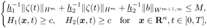
if we define $\phi _\ell :=\boldsymbol {l}_\ell (H_\ell )\cdot \boldsymbol {\phi }_\ell$ for $\ell =1,2$
 , then $(\zeta,\phi _1,\phi _2)$
 satisfy approximately the full model for interfacial gravity waves as

Here, the errors $(\mathfrak {r}_1,\mathfrak {r}_2,\mathfrak {r}_0)$ satisfy

for $t\in [0,T]$ .
.
Particularly, we see that under the special choice of indices (H1) or (H2), the solutions to the Kakinuma model (2.18)–(2.20) constructed in theorem 3.1 satisfy approximately the full model for interfacial gravity waves (2.17) with the choice $\phi _\ell =\boldsymbol {l}_\ell (H_\ell )\cdot \boldsymbol {\phi }_\ell$ $(\ell =1,2)$
 and that the error is of order $O((\underline {h}_1\delta )^{4N+2}+(\underline {h}_2\delta )^{4N+2})$
 .
.
Conversely, the next theorem shows that the full model for interfacial gravity waves is consistent with the Kakinuma model at order $O((\underline {h}_1\delta )^{4N+2}+(\underline {h}_2\delta )^{4N+2})$ under the special choice of indices (H1) or (H2).
Theorem 3.6 Let $c, M$ be positive constants and $m$
 an integer such that $m \geq 4(N+1)$
 and $m>\frac {n}{2}+1$
 . We assume (H1) or (H2). There exists a positive constant $C$
 such that for any positive parameters $\underline {\rho }_1, \underline {\rho }_2, \underline {h}_1, \underline {h}_2, \delta$
 satisfying $\underline {h}_1\delta, \underline {h}_2\delta \leq 1$
 and for any solution $(\zeta,\phi _1,\phi _2)$
 to the full model for interfacial gravity waves (2.17) on a time interval $[0,T]$
 with a bottom topography $b\in W^{m+1,\infty }$
 satisfying (3.18), if we define $H_1$
 and $H_2$
 as in (2.19) and $\boldsymbol {\phi }_1$
 and $\boldsymbol {\phi }_2$
 as the unique solutions to the problems

then $(\zeta,\boldsymbol {\phi }_1,\boldsymbol {\phi }_2)$ satisfy approximately the Kakinuma model as

Here, the errors $(\tilde {\boldsymbol {\mathfrak {r}}}_1,\tilde {\boldsymbol {\mathfrak {r}}}_2,\tilde {\mathfrak {r}}_0)$ satisfy

for $t\in [0,T]$ .
.
Remark 3.7 The unique existence of the solutions $\boldsymbol {\phi }_1$ and $\boldsymbol {\phi }_2$
 to the problems (3.19) is guaranteed by lemma 4.4 below under an additional assumption $\phi _1(\cdot,t),\phi _2(\cdot,t) \in \mathring {H}^m$
 . Lemma 4.4 is essentially a simple corollary of [Reference Iguchi19, lemma 3.4].
Remark 3.8 In order to define the approximate solution $(\boldsymbol {\phi }_1,\boldsymbol {\phi }_2)$ to the Kakinuma model (2.18) from the solution $(\zeta,\phi _1,\phi _2)$
 to the full model, we can use, in place of (3.19), the following system of equations
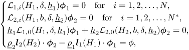
where $\phi =\underline {\rho }_2\phi _2-\underline {\rho }_1\phi _1$ is the canonical variable for the full model for interfacial gravity waves. The above system is nothing but the compatibility conditions (3.7) together with the definition (3.17) of the canonical variable for the Kakinuma model. The existence of the approximate solution $(\boldsymbol {\phi }_1,\boldsymbol {\phi }_2)$
 is guaranteed by lemma 5.1 given in § 5. Then, we have similar error estimates to (3.20). For details, we refer to proposition 7.6.
The above theorems 3.5 and 3.6 concern essentially the approximation of the equations. To give a rigorous justification of the Kakinuma model (2.18) as a higher order shallow water approximation to the full model for interfacial gravity waves (2.17), one needs to give an error estimate between solutions to the Kakinuma model and that to the full model. However, we cannot expect to construct general solutions to the initial value problem for the full model for interfacial gravity waves because the initial value problem is ill-posed. Nevertheless, if we assume the existence of a solution to the full model with a uniform bound with respect to the shallowness parameters $\delta _1=\underline {h}_1\delta$ and $\delta _2=\underline {h}_2\delta$
 , then we can give an error estimate with respect to a solution to the Kakinuma model by making use of the well-posedness of the initial value problem for the Kakinuma model as we can see in the following theorem.
Theorem 3.9 Let $c, M, \underline {h}_\mathrm {min}$ be positive constants and $m$
 an integer such that ${m>\frac {n}{2}+4(N+1)}$
 . We assume (H1) or (H2). Then, there exist a time $T>0$
 and a constant $C>0$
 such that the following holds true. Let $\underline {\rho }_1, \underline {\rho }_2, \underline {h}_1, \underline {h}_2, \delta$
 be positive parameters satisfying the natural restrictions (2.14), $\underline {h}_1\delta, \underline {h}_2\delta \leq 1$
 , and the condition ${\underline {h}_\mathrm {min} \leq \underline {h}_1, \underline {h}_2}$
 , and let $b\in W^{m+2,\infty }$
 such that $\underline {h}_2^{-1}\|b\|_{W^{m+2,\infty }}\leq M$
 . Suppose that the full model for interfacial gravity waves (2.17) possesses a solution $(\zeta ^{\text {IW}},\phi _1^{{\rm IW}},\phi _2^{{\rm IW}}) \in C([0,T^{\text {IW}}];H^{m+1}\times \mathring {H}^{m+1}\times \mathring {H}^{m+1})$
 satisfying a uniform bound

where we denote $H_1^{{\rm IW}}:=1-\underline {h}_1^{-1}\zeta ^{{\rm IW}}$ and $H_2^{{\rm IW}}:=1+\underline {h}_2^{-1}\zeta ^{{\rm IW}}-\underline {h}_2^{-1}b$
 . Let $\zeta _{(0)}:=\zeta ^{{\rm IW}}|_{t=0}$
 and $\phi _{(0)}:=(\underline {\rho }_2\phi _2^{{\rm IW}}-\underline {\rho }_1\phi _1^{{\rm IW}})|_{t=0}$
 be the initial data for the canonical variables, and let $(\boldsymbol {\phi }_{1(0)},\boldsymbol {\phi }_{2(0)})$
 be the initial data to the Kakinuma model constructed from $(\zeta _{(0)},\phi _{(0)})$
 by proposition 3.4. Assume moreover that the initial data $(\zeta _{(0)},\boldsymbol {\phi }_{1(0)},\boldsymbol {\phi }_{2(0)})$
 satisfy the stability condition (3.12), let $(\zeta ^{{\rm K}}, \boldsymbol {\phi }_1^{{\rm K}},\boldsymbol {\phi }_2^{{\rm K}})$
 be the solution to the initial value problem for the Kakinuma model (2.18)–(2.20) on the time interval $[0,T]$
 whose unique existence is guaranteed by theorem 3.1, and put $\phi _\ell ^{{\rm K}}=\boldsymbol {l}_\ell (H_\ell )\cdot \boldsymbol {\phi }_\ell ^{{\rm K}}$
 for $\ell =1,2$
 . Then, we have the error bound

for $0\leq t\leq \min \{T,T^{{\rm IW}}\}$ .
.
The next theorem is the final main result in this paper and states the consistency of the Hamiltonian $\mathscr {H}^{{\tiny K}}(\zeta,\phi )$ of the Kakinuma model with respect to the Hamiltonian $\mathscr {H}^{{\rm IW}}(\zeta,\phi )$
 of the full model for interfacial gravity waves. We recall that these Hamiltonians are defined in (2.25) and (2.22), respectively.
Theorem 3.10 Let $c, M, \underline {h}_\mathrm {min}$ be positive constants and $m$
 an integer such that $m>\frac {n}{2}+1$
 and $m \geq 4(N+1)$
 . We assume (H1) or (H2). There exists a positive constant $C$
 such that for any positive parameters $\underline {\rho }_1, \underline {\rho }_2, \underline {h}_1, \underline {h}_2, \delta$
 satisfying the natural restrictions (2.14), $\underline {h}_1\delta, \underline {h}_2\delta \leq 1$
 , and the condition ${\underline {h}_\mathrm {min} \leq \underline {h}_1, \underline {h}_2}$
 , and for any $(\zeta,\phi )\in H^m\times \mathring {H}^{4(N+1)}$
 and $b\in W^{m+1,\infty }$
 satisfying

with $H_1$ and $H_2$
 defined by (2.19), we have

4. Consistency of the Kakinuma model; proof of theorems 3.5 and 3.6
In this section, we show that under the special choice of the indices $p_0,p_1,\ldots, p_{N^*}$ as
as
(H1) $N^*=N$
and $p_i=2i$ $(i=0,1,\ldots,N)$ in the case of the flat bottom $b(\boldsymbol {x})\equiv 0$,(H2) $N^*=2N$
and $p_i=i$ $(i=0,1,\ldots,2N)$ in the case with general bottom topographies,


the Kakinuma model (2.18)is a higher order model to the full model for interfacial gravity waves (2.17) in the limit ${\delta _1=\underline {h}_1\delta \to 0}$ , ${\delta _2=\underline {h}_2\delta \to 0}$
 , in the sense of consistency. Specifically, we prove theorems 3.5 and 3.6. Our proof relies essentially on results obtained in the framework of surface waves in [Reference Iguchi19], which are recalled in § 4.1. The extension to the framework of interfacial waves and the completion of the proof are provided in § 4.2.
4.1. Results in the framework of surface waves
In this subsection, we consider the case of surface waves where the water surface and the bottom of the water are represented as $z=\zeta (\boldsymbol {x})$ and $z=-1+b(\boldsymbol {x})$
 , respectively. Here, the time $t$
 is fixed arbitrarily, so that we omit the dependence of $t$
 in notations. Let $H(\boldsymbol {x})=1+\zeta (\boldsymbol {x})-b(\boldsymbol {x})$
 be the water depth. For a non-negative integer $N$
 , let $N^*$
 and $p_0,p_1,\ldots,p_{N^*}$
 be non-negative integers satisfying the condition (H1) or (H2). Put

and define $L_{ij} = L_{ij}(H,b,\delta )$ $(i,j=0,1,\ldots,N^*)$
 by
by

where we use the notational convention $0/0 = 0$ . Introduce linear operators $\mathcal {L}_{i} = \mathcal {L}_{i}(H,b,\delta )$ $(i=0,1,\ldots,N^*)$
 acting on ${\boldsymbol \varphi } = (\varphi _{0},\ldots,\varphi _{N^*})^\mathrm {T}$
 by
by
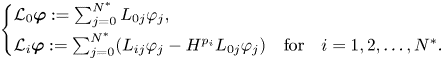
The following lemma has been proved in [Reference Iguchi19, lemmas 3.2 and 3.4].
Lemma 4.1 Let $c, M$ be positive constants and $m$
 an integer such that $m>\frac {n}{2}+1$
 . There exists a positive constant $C$
 such that if $\zeta \in H^m$
 , $b\in W^{m,\infty }$
 and $H=1+\zeta -b$
 satisfy

then for any $k=\pm 0,\dots, \pm (m-1)$ , any $\delta \in (0,1]$
 and any $\phi \in \mathring {H}^{k+1}$
 , there exists a unique solution $\boldsymbol {\phi }=(\phi _0,\phi _1,\ldots,\phi _{N^*})=(\phi _0,\boldsymbol {\phi }')\in \mathring {H}^{k+1}\times (H^{k+1})^{N^*}$
 to the problem
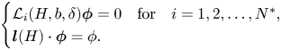
Moreover, the solution satisfies $\|\nabla \boldsymbol {\phi }\|_{H^k} + \delta ^{-1}\|\boldsymbol {\phi }'\|_{H^k} \leq C\|\nabla \phi \|_{H^k}$ .
.
As a corollary of this lemma, under the assumptions of lemma 4.1
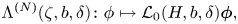
where $\boldsymbol {\phi }$ is the unique solution to (4.5), is defined as a bounded linear operator from $\mathring {H}^{k+1}$
 to $H^{k-1}$
 for any $k=\pm 0,\dots, \pm (m-1)$
 . A key result is that the operator $\Lambda ^{(N)}(\zeta,b,\delta )$
 provides good approximations in the shallow water regime $\delta \ll 1$
 to the corresponding Dirichlet-to-Neumann map $\Lambda (\zeta,b,\delta )$
 , which is defined by

where $\Phi$ is the unique solution to the boundary value problem
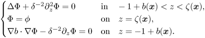
More precisely, we have the following lemma.
Lemma 4.2 Let $c, M$ be positive constants and $m, j$
 integers such that $m>\frac {n}{2}+1$
 , $m\geq 2(j+1)$
 and $1\leq j\leq 2N+1$
 . We assume (H1) or (H2). There exists a positive constant $C$
 such that if $\zeta \in H^m$
 , $b\in W^{m+1,\infty }$
 and $H=1+\zeta -b$
 satisfy

then for any $\phi \in \mathring {H}^{k+2(j+1)}$ with $0\leq k\leq m-2(j+1)$
 and any $\delta \in (0,1]$
 we have

Proof. We observe that the bound on $\mathfrak {r}_1:=\Lambda ^{(N)}(\zeta,b,\delta )\phi -\Lambda (\zeta,b,\delta )\phi$ in the case $j=2N+1$
 and $k=m-4(N+1)$
 is given in [Reference Iguchi19, theorem 2.2] and proved in [Reference Iguchi19, § 8.1 and 8.2]. The proof is also valid in the case $1\leq j\leq 2N+1$
 and $0\leq k\leq m-2(j+1)$
 .
.
The above estimate allows us to obtain the desired consistency result on the equations describing the conservation of mass. We need a similar estimate for the contributions of Bernoulli's equation. To this end, we denote

and

with

where ${\boldsymbol l}^\prime (H) := (0,p_1 H^{p_1-1},\ldots,p_{N^*}H^{p_{N^*}-1})^\mathrm {T}$ and ${\boldsymbol \phi } := (\phi _0,\phi _1,\ldots,\phi _{N^*})^\mathrm {T}$
 is the solution to (4.5), whose unique existence is guaranteed by lemma 4.1. Then, the following lemma shows that $B^{(N)}(\phi ;\zeta,b,\delta )$
 is a higher order approximation to $B(\phi ;\zeta,b,\delta )$
 in the shallow water regime $\delta \ll 1$
 .
.
Lemma 4.3 Let $c, M$ be positive constants and $m$
 an integer such that ${m\geq 4(N+1)}$
 and $m>\frac {n}{2}+1$
 . We assume (H1) or (H2). There exists a positive constant $C$
 such that if $\zeta \in H^m$
 , $b\in W^{m+1,\infty }$
 and $H=1+\zeta -b$
 satisfy (4.8), then for any $\phi \in \mathring {H}^m$
 and any $\delta \in (0,1]$
 we have

Proof. Notice first that differentiating $\phi =\boldsymbol {l}(H)\cdot \boldsymbol {\phi }$ we have $\nabla \phi ={\boldsymbol u}+ w\nabla \zeta$
 , so that

If we introduce a residual $\mathfrak {r}$ by
by

where $\Phi$ is the solution to the boundary value problem (4.7) and $\Phi ^\mathrm {app}$
 is an approximate velocity potential defined by

then we have $\mathfrak {r}=\delta ^{-2}w-\nabla \zeta \cdot \boldsymbol {u}-\Lambda (\zeta,b,\delta )\phi =\delta ^{-2} w(1+\delta ^2|\nabla \zeta |^2)-\nabla \zeta \cdot \nabla \phi -\Lambda (\zeta,b,\delta )\phi$ . Therefore, we obtain

The desired estimate for the second term readily follows from lemmas 4.1 and 4.2. As for the first term, in view of $m>\frac {n}{2}$ we can use a calculus inequality $\|\mathfrak {r}^2\|_{H^k} \lesssim \|\mathfrak {r}\|_{H^{(m+k)/2}}^2$
 for $k\in \{0,1,\dots,m\}$
 . Particularly, we have $\|\mathfrak {r}^2\|_{H^{m-4(N+1)}} \lesssim \|\mathfrak {r}\|_{H^{m-2(N+1)}}^2$
 . The last term can be evaluated by estimates in [Reference Iguchi19, § 8.1 and 8.2].
4.2 Results in the framework of interfacial waves
In this section, we prove theorems 3.5 and 3.6. To this end, we first rewrite the Kakinuma model (2.18) using a formulation which allows a direct comparison with the full model for interfacial gravity waves (2.17), thanks to the following lemma.
Lemma 4.4 Let $c, M$ be positive constants and $m$
 an integer such that $m>\frac {n}{2}+1$
 . There exists a positive constant $C$
 such that for any positive parameters $\underline {h}_1, \underline {h}_2, \delta$
 satisfying $\underline {h}_1\delta, \underline {h}_2\delta \leq 1$
 , if $\zeta \in H^m$
 , $b\in W^{m,\infty }$
 , $H_1 = 1 - \underline {h}_1^{-1}\zeta$
 and $H_2 = 1 + \underline {h}_2^{-1}\zeta - \underline {h}_2^{-1}b$
 satisfy

then for any $k=0,\pm 1,\ldots,\pm (m-1)$ and any $\phi _1,\phi _2 \in \mathring {H}^{k+1}$
 there exists a unique solution $\boldsymbol {\phi }_1=(\phi _{1,0},\boldsymbol {\phi }_1')\in \mathring {H}^{k+1}\times (H^{k+1})^N$
 , $\boldsymbol {\phi }_2=(\phi _{2,0},\boldsymbol {\phi }_2')\in \mathring {H}^{k+1}\times (H^{k+1})^{N^*}$
 to the problem

Moreover, the solution satisfies $\|\nabla \boldsymbol {\phi }_\ell \|_{H^k} + (\underline {h}_\ell \delta )^{-1}\|\boldsymbol {\phi }_\ell '\|_{H^k} \leq C\|\nabla \phi _\ell \|_{H^k}$ for $\ell =1,2$
 .
.
Proof. Notice that we have identities

with suitable choices of indices $\{p_i\}$ . Hence, lemma 4.1 gives the desired result.
As a corollary of this lemma, under the assumptions of lemma 4.4

where $(\boldsymbol {\phi }_1,\boldsymbol {\phi }_2)$ is the unique solution to (4.12), are defined as bounded linear operators from $\mathring {H}^{k+1}$
 to $H^{k-1}$
 for any $k=\pm 0,\dots, \pm (m-1)$
 . Using these definitions and noting the relations (3.8) and $\boldsymbol {l}_\ell (H_\ell )\cdot \partial _t\boldsymbol {\phi }_\ell = \partial _t(\boldsymbol {l}_\ell (H_\ell )\cdot \boldsymbol {\phi }_\ell )-w_\ell \underline {h}_\ell ^{-1}\partial _t\zeta$
 , we can transform the Kakinuma model (2.18) equivalently as

where we recall that ${\boldsymbol u}_1$ , ${\boldsymbol u}_2$
 , $w_1$
 and $w_2$
 are uniquely determined from $\phi _1$
 and $\phi _2$
 by (3.4), wherein ${\boldsymbol \phi }_1$
 and ${\boldsymbol \phi }_2$
 are defined as the solutions to (4.12).
We further introduce notations, which are contributions of Bernoulli's equation and interfacial versions of $B$ and $B^{(N)}$
 defined by (4.9) and (4.10). We denote

and

Then, the full model for interfacial gravity waves (2.17) and the Kakinuma model (4.13) can be written simply as

and

respectively. The following lemmas show that $\underline {h}_1\Lambda _1^{(N)}$ , $\underline {h}_2\Lambda _2^{(N)}$
 , $B_1^{(N)}$
 and $B_2^{(N)}$
 are higher order approximations in the shallow water regime $\delta _1=\underline {h}_1\delta \ll 1$
 and $\delta _2=\underline {h}_2\delta \ll 1$
 to $\Lambda _1$
 , $\Lambda _2$
 , $B_1$
 and $B_2$
 , respectively.
Lemma 4.5 Let $c, M$ be positive constants and $m, j$
 integers such that $m>\frac {n}{2}+1$
 , $m\geq 2(j+1)$
 and $1\leq j\leq 2N+1$
 . We assume (H1) or (H2). There exists a positive constant $C$
 such that for any positive parameters $\underline {h}_1, \underline {h}_2, \delta$
 satisfying $\underline {h}_1\delta, \underline {h}_2\delta \leq 1$
 , if $\zeta \in H^m$
 , $b\in W^{m+1,\infty }$
 , $H_1 = 1 - \underline {h}_1^{-1}\zeta$
 and $H_2 = 1 + \underline {h}_2^{-1}\zeta - \underline {h}_2^{-1}b$
 satisfy

then for any $\phi _1,\phi _2 \in \mathring {H}^{k+2(j+1)}$ with $0\leq k\leq m-2(j+1)$
 we have
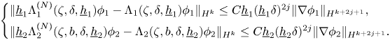
Proof. By simple scaling arguments, we have
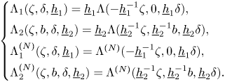
Therefore, the results follow from lemma 4.2.
Lemma 4.6 Let $c, M$ be positive constants and $m$
 an integer such that ${m\geq 4(N+1)}$
 and $m>\frac {n}{2}+1$
 . We assume (H1) or (H2). There exists a positive constant $C$
 such that for any positive parameters $\underline {h}_1, \underline {h}_2, \delta$
 satisfying $\underline {h}_1\delta, \underline {h}_2\delta \leq 1$
 , if $\zeta \in H^m$
 , $b\in W^{m+1,\infty }$
 , $H_1 = 1 - \underline {h}_1^{-1}\zeta$
 and $H_2 = 1 + \underline {h}_2^{-1}\zeta - \underline {h}_2^{-1}b$
 satisfy (4.14), then for any $\phi _1,\phi _2 \in \mathring {H}^m$
 we have

Proof. By simple scaling arguments, we have

Therefore, the results follow from lemma 4.3.
We can now prove theorems 3.5 and 3.6. In view of (3.8) the errors $(\mathfrak {r}_1,\mathfrak {r}_2,\mathfrak {r}_0)$ and $(\tilde {\boldsymbol {\mathfrak {r}}}_1,\tilde {\boldsymbol {\mathfrak {r}}}_2, \tilde {\mathfrak {r}}_0)$
 can be written explicitly as

Therefore, the theorems are simple corollaries of the above lemmas 4.5 and 4.6.
5. Elliptic estimates and time derivatives
In this section, we derive useful uniform a priori bounds on regular solutions to the Kakinuma model (2.18). Firstly, due to the fact that the hypersurface $t=0$ in the space-time $\mathbf {R}^n\times \mathbf {R}$
 is characteristic for the Kakinuma model, we need the following key elliptic estimate in order to be able to estimate time derivatives of the solution. Let us recall that the operators $\mathcal {L}_{1,i}$
 for $i=0,1,\ldots,N$
 and $\mathcal {L}_{2,i}$
 for $i=0,1,\ldots,N^*$
 are defined by (3.6), and the vectors $\boldsymbol {l}_1(H_1)$
 and $\boldsymbol {l}_2(H_2)$
 are defined by (3.3). We recall the convention that for a vector ${\boldsymbol \phi }=(\phi _0,\phi _1,\ldots,\phi _N)^\mathrm {T}$
 we denote the last $N$
 components by ${\boldsymbol \phi }'=(\phi _1,\ldots,\phi _N)^\mathrm {T}$
 .
.
Lemma 5.1 Let $c, M$ be positive constants and $m$
 an integer such that $m>\frac {n}{2}+1$
 . There exists a positive constant $C$
 such that for any positive parameters $\underline {\rho }_1, \underline {\rho }_2, \underline {h}_1, \underline {h}_2, \delta$
 satisfying $\underline {h}_1\delta, \underline {h}_2\delta \leq 1$
 , if $\zeta \in H^m$
 , $b\in W^{m,\infty }$
 , $H_1 = 1 - \underline {h}_1^{-1}\zeta$
 and $H_2 = 1 + \underline {h}_2^{-1}\zeta - \underline {h}_2^{-1}b$
 satisfy (4.11), then for any $\boldsymbol {f}_1' = (f_{1,1},\ldots,f_{1,N})^\mathrm {T} \in (H^{k})^N$
 , $\boldsymbol {f}_2' = (f_{2,1},\ldots,$ $f_{2,N^*})^\mathrm {T} \in (H^{k})^{N^*}$
 , $\boldsymbol {f}_3 \in (H^k)^n$
 and $f_4\in \mathring H^{k+1}$
 with $k\in \{0,1,\ldots,m-1\}$
 , there exists a solution $(\boldsymbol {\varphi }_1,\boldsymbol {\varphi }_2)$
 to
to
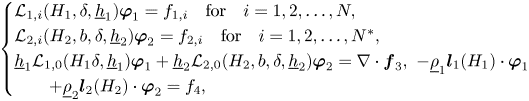
satisfying

Moreover, the solution is unique up to an additive constant of the form $(\mathcal {C}\underline {\rho }_2,\mathcal {C}\underline {\rho }_1)$ to $(\varphi _{1,0},\varphi _{2,0})$
 .
.
Proof. The existence and uniqueness up to an additive constant of the solution has been given in the companion paper [Reference Duchêne and Iguchi14, lemma 6.4]. We focus here on the derivation of uniform estimates. By direct rescaling within the proof of [Reference Duchêne and Iguchi14, lemma 6.1], we infer that

for $\ell =1,2$ . We note the identities

so that for the solution $(\boldsymbol {\varphi }_1,\boldsymbol {\varphi }_2)$ to (5.1) we have

Therefore, it is sufficient to evaluate $I_1$ and $I_2$
 . As for the term $I_2$
 we have

As for the term $I_1$ , we note the trivial identities

Therefore, the term $I_1$ in (5.2) can be expressed in two ways as

By the linearity of (5.1) it is sufficient to evaluate it in the case $f_4=0$ and in the case $\boldsymbol {f}_3=\boldsymbol {0}$
 , separately. In the case $f_4=0$
 , we evaluate it as

In the case $\boldsymbol {f}_3=\boldsymbol {0}$ , we evaluate it as

From the above estimates, we deduce immediately the desired inequality for $k=0$ .
.
In order to obtain the desired inequality on derivatives, we let $k\in \{1,2,\ldots, m-1\}$ and $\beta$
 be a multi-index such that $1\leq |\beta |\leq k$
 . Applying the differential operator $\partial ^\beta$
 to (5.1), we have

where
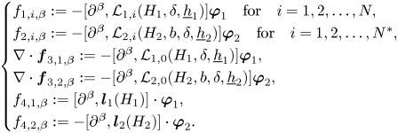
We put $\boldsymbol {f}_{1,\beta }=(0,f_{1,1,\beta },\ldots,f_{1,N,\beta })$ and $\boldsymbol {f}_{2,\beta }=(0,f_{2,1,\beta },\ldots,f_{2,N^*,\beta })$
 . Then, with a suitable decomposition $\boldsymbol {f}_{\ell,\beta } = \boldsymbol {f}_{\ell,\beta }^\mathrm {high} + \boldsymbol {f}_{\ell,\beta }^\mathrm {low}$
 for $\ell =1,2$
 , we see that

for $\ell =1,2$ . Therefore, in view of the linearity of (5.1), the desired inequality for $k\geq 1$
 follows by induction on $k$
 .
.
From the above elliptic estimates, we deduce the following bounds on time derivatives of regular solutions to the Kakinuma model (2.18). We introduce a mathematical energy $E_m(t)$ for a solution $(\zeta,\boldsymbol {\phi }_1,\boldsymbol {\phi }_2)$
 to the Kakinuma model by

where $\boldsymbol {\phi }_1'=(\phi _{1,1},\ldots,\phi _{1,N})^\mathrm {T}$ and $\boldsymbol {\phi }_2'=(\phi _{2,1},\ldots,\phi _{2,N^*})^\mathrm {T}$
 .
.
Lemma 5.2 Let $c, M_1, \underline {h}_\mathrm {min}$ be positive constants and $m$
 an integer such that $m>\frac {n}{2}+1$
 . There exists a positive constant $C_1$
 such that for any positive parameters $\underline {\rho }_1, \underline {\rho }_2, \underline {h}_1, \underline {h}_2, \delta$
 satisfying the natural restrictions (2.14), $\underline {h}_1\delta, \underline {h}_2\delta \leq 1$
 , and the condition $\underline {h}_\mathrm {min} \leq \underline {h}_1,\underline {h}_2$
 , if a regular solution $(\zeta,\boldsymbol {\phi }_1,\boldsymbol {\phi }_2)$
 to the Kakinuma model (2.18) with bottom topography $b\in W^{m+1,\infty }$
 satisfy

then we have
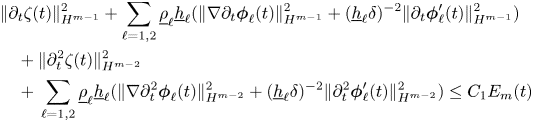
for $0\leq t\leq T$ .
.
Proof. First, we recall that the Kakinuma model (2.18) can be written compactly as (3.5). It follows from the first component of the first two equations in (3.5) that $\partial _t\zeta$ can be written in two ways as $\partial _t\zeta =-\underline {h}_1\mathcal {L}_{1,0}\boldsymbol {\phi }_1=\underline {h}_2\mathcal {L}_{2,0}\boldsymbol {\phi }_2$
 , so that

where we used (2.15).
As for the estimate of $(\partial _t\boldsymbol {\phi }_1,\partial _t\boldsymbol {\phi }_2)$ , we differentiate the compatibility conditions (3.7) with respect to time and use the last equation in (3.5). Then, we have
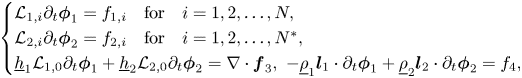
where

Therefore, by lemma 5.1 we have
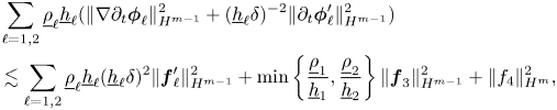
where $\boldsymbol {f}_1'=(f_{1,1},\ldots,f_{1,N})^\mathrm {T}$ , $\boldsymbol {f}_2'=(f_{2,1},\ldots,f_{2,N^*})^\mathrm {T}$
 , and we used (2.15). We proceed to evaluate the right-hand side. By writing down the operators $\mathcal {L}_{\ell,i}$
 explicitly, we see that the operators do not include any derivatives of $H_{\ell }$
 . Therefore, we can write $f_{\ell,i}$
 as
as

We note also that the differential operators $\frac {\partial }{\partial H_\ell }\mathcal {L}_{\ell,i}$ have a similar structure as $\mathcal {L}_{\ell,i}$
 . Therefore,

where, here and henceforth, we utilize fully our restriction $\underline {h}_1^{-1},\underline {h}_2^{-1} \lesssim 1$ . In view of the definition (3.4) of $\boldsymbol {u}_1, \boldsymbol {u}_2,w_1$
 and $w_2$
 , we see easily that

We evaluate the term on $\boldsymbol {f}_3$ as
as

Similarly, we have

Plugging in (5.7) the above estimates, we obtain the desired estimate for $(\partial _t\boldsymbol {\phi }_1,\partial _t\boldsymbol {\phi }_2)$ .
.
Finally, the estimate of $\partial _t^2\zeta$ can be obtained by differentiating $\partial _t\zeta =-\underline {h}_1\mathcal {L}_{1,0}\boldsymbol {\phi }_1=\underline {h}_2\mathcal {L}_{2,0}\boldsymbol {\phi }_2$
 with respect to time. Then, the estimate of $(\partial _t^2\boldsymbol {\phi }_1,\partial _t^2\boldsymbol {\phi }_2)$
 can be obtained by differentiating (5.5) with respect to time once more and applying lemma 5.1.
Remark 5.3 In view of the above arguments, we see easily that for the Kakinuma model (2.18), $(\partial _t\boldsymbol {\phi }_1, \partial _t\boldsymbol {\phi }_2)|_{t=0}$ can be determined from the initial data $(\zeta _{(0)},\boldsymbol {\phi }_{1(0)},\boldsymbol {\phi }_{2(0)})$
 and the bottom topography $b$
 , although the hypersurface $t=0$
 is characteristic for the model. They are unique up to an additive constant of the form $(\mathcal {C}\underline {\rho }_2,\mathcal {C}\underline {\rho }_1)$
 to $(\partial _t\phi _{1,0},\partial _t\phi _{2,0})|_{t=0}$
 . Particularly, $(\partial _t\boldsymbol {\phi }_1', \partial _t\boldsymbol {\phi }_2')|_{t=0}$
 and hence $a|_{t=0}$
 with the function $a$
 given in (3.9) can be uniquely determined from the data.
6. Uniform energy estimates; proof of theorem 3.1
In this section, we provide uniform energy estimates for solutions to the Kakinuma model. Consequently, we prove theorem 3.1. We recall that the Kakinuma model (2.18) can be written compactly as
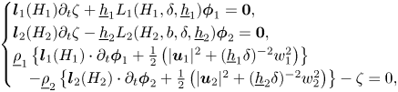
where we recall that $H_1 := 1 - \underline {h}_1^{-1}\zeta$ , $H_2:= 1 + \underline {h}_2^{-1}\zeta - \underline {h}_2^{-1}b$
 , ${\boldsymbol \phi }_1 := (\phi _{1,0},\phi _{1,1},\ldots, \phi _{1,N})^\mathrm {T}$
 , ${\boldsymbol \phi }_2 := (\phi _{2,0},\phi _{2,1},\ldots,\phi _{2,N^*})^\mathrm {T}$
 , and ${\boldsymbol l}_1$
 , ${\boldsymbol l}_2$
 , $L_1$
 , $L_2$
 , ${\boldsymbol u}_1$
 , ${\boldsymbol u}_2$
 , $w_1$
 , $w_2$
 are defined in § 3.
6.1 Analysis of linearized equations
Before deriving linearized equations to the Kakinuma model (6.1), we introduce some more notations. For $\ell =1,2$ , the coefficient matrices of the principal part and the singular part with respect to the small parameter $\delta _\ell =\underline {h}_\ell \delta$
 of the operator $L_{\ell }$
 are denoted by $A_\ell (H_\ell )$
 and $C_\ell (H_\ell )$
 , respectively, that is,

and

We put also

In the above expressions, we used the notational convention $0/0 = 0$ . Then, the operators $L_1$
 and $L_2$
 can also be written as

For $\ell =1,2$ , we decompose the operator $L_\ell$
 as $L_\ell =L_\ell ^\mathrm {pr}+L_\ell ^\mathrm {low}$
 , where

We now linearize the Kakinuma model (6.1) around an arbitrary flow $(\zeta,\boldsymbol {\phi }_1,\boldsymbol {\phi }_2)$ and denote the variation by $(\dot {\zeta },\dot {\boldsymbol {\phi }}_1,\dot {\boldsymbol {\phi }}_2)$
 . After neglecting lower order terms, the linearized equations have the form

where the function $a$ is defined by (3.9). In order to derive a good symmetric structure of the equations, following the companion paper [Reference Duchêne and Iguchi14] we introduce
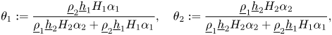
where

for $\ell =1,2$ and $\boldsymbol {1}:=(1,\ldots,1)^\mathrm {T}$
 . Then, we have $\theta _1+\theta _2=1$
 . We recall that $\alpha _1$
 and $\alpha _2$
 are positive constants depending only on $N$
 and the non-negative integers $0=p_0< p_1<\ldots < p_{N^*}$
 , respectively, and go to $0$
 as $N,N^*\to \infty$
 . We also introduce

Then, we have $\boldsymbol {u}_1=\boldsymbol {u}-\theta _1\boldsymbol {v}$ and $\boldsymbol {u}_2=\boldsymbol {u}+\theta _2\boldsymbol {v}$
 . Plugging these into the linearized equations (6.7), we can write them in a matrix form as

where

and
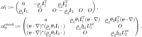
Here, $(\boldsymbol {v}\cdot \nabla )^*$ denotes the adjoint operator of $\boldsymbol {v}\cdot \nabla$
 in $L^2$
 , that is, $(\boldsymbol {v}\cdot \nabla )^*f=-\nabla \cdot (f\boldsymbol {v})$
 . We note that $\mathscr {A}_1$
 is a skew-symmetric matrix and $\mathscr {A}_0^\mathrm {mod}$
 is symmetric in $L^2$
 . Therefore, the corresponding energy function is given by $(\mathscr {A}_0^\mathrm {mod}\dot {\boldsymbol {U}},\dot {\boldsymbol {U}})_{L^2}$
 . We put

The following lemma shows that $(\mathscr {A}_0^\mathrm {mod}\dot {U},\dot {U})_{L^2} \simeq \mathscr {E}(\dot {\boldsymbol {U}})$ under the non-cavitation assumption and the stability condition, stated respectively as (3.11) and (3.12) in theorem 3.1.
Lemma 6.1 Let $c, M, \underline {h}_\mathrm {min}$ be positive constants. There exists a positive constant $C$
 such that for any positive parameters $\underline {\rho }_1,\underline {\rho }_2,\underline {h}_1,\underline {h}_2,\delta$
 satisfying the condition $\underline {h}_\mathrm {min} \leq \underline {h}_1,\underline {h}_2$
 , if $H_1,H_2,\boldsymbol {u}_1,\boldsymbol {u}_2$
 and the function $a$
 satisfy
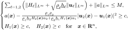
then for any $\dot {\boldsymbol {U}} = (\dot {\zeta },\dot {\boldsymbol {\phi }}_1,\dot {\boldsymbol {\phi }}_2)^\mathrm {T} \in L^2\times (\mathring {H}^1\times (H^1)^N)\times (\mathring {H}^1\times (H^1)^{N^*})$ we have

Proof. This lemma can be shown along with the proof of [Reference Duchêne and Iguchi14, lemma 7.4]. For the sake of completeness, we sketch the proof. We first note that

where we used the identity $\boldsymbol {a}\cdot (\boldsymbol {v}\cdot \nabla )\boldsymbol {\varphi } = \boldsymbol {v}\cdot (\boldsymbol {a}\otimes \nabla )^\mathrm {T}\boldsymbol {\varphi }$ . On the other hand, we can put

for $\ell =1,2$ . Then, we see that $q_\ell (H_\ell )=H_\ell \alpha _\ell$
 and that $Q_\ell (H_\ell )$
 is non-negative. Moreover, the identity

holds for any $\boldsymbol {\varphi }_\ell$ . Therefore,

so that

We proceed to evaluate $I_1$ .
.

where the matrix $\mathfrak {A}_0$ is given by

Here, we see that

so that $\mathfrak {A}_0$ is positive definite by Sylvester's criterion. Moreover, $\operatorname {tr}\mathfrak {A}_0 \leq \max \{1,\alpha _1,\alpha _2\}\, M \lesssim 1$
 and the minimal eigenvalue of the matrix $\mathfrak {A}_0$
 is bounded from below by $4\det \mathfrak {A}_0/(\operatorname {tr}\mathfrak {A}_0)^2 \gtrsim 1$
 . Therefore, we obtain

As for $I_2$ , it is easy to see that $(C_\ell \dot {\boldsymbol {\phi }}_\ell,\dot {\boldsymbol {\phi }}_\ell )_{L^2} \simeq \|\dot {\boldsymbol {\phi }}_\ell '\|_{L^2}^2$
 for $\ell =1,2$
 . Summarizing the above estimates and using the decomposition (6.13) again, we obtain $(\mathscr {A}_0^\mathrm {mod}\dot {\boldsymbol {U}},\dot {\boldsymbol {U}})_{L^2} \gtrsim \mathscr {E}(\dot {\boldsymbol {U}})$
 .
.
In order to obtain the estimate of $(\mathscr {A}_0^\mathrm {mod}\dot {\boldsymbol {U}},\dot {\boldsymbol {U}})_{L^2}$ from above, it is sufficient to show that each element of the matrix $\mathfrak {A}_0$
 is uniformly bounded. Since $\theta _1+\theta _2=1$
 , we have

Here, we see that

Similarly, we have $\sqrt {\underline {\rho }_2/\underline {h}_2} \theta _2|\boldsymbol {u}_1| \lesssim 1$ . Therefore, we obtain $(\mathscr {A}_0^\mathrm {mod}\dot {\boldsymbol {U}},\dot {\boldsymbol {U}})_{L^2} \lesssim \mathscr {E}(\dot {\boldsymbol {U}})$
 .
.
In the following lemma we provide uniform energy estimates for regular solutions to the linearized Kakinuma model (6.7).
Proposition 6.2 Let $c,M,M_1,\underline {h}_\mathrm {min}$ be positive constants. There exist positive constants $C=C(c,M,\underline {h}_\mathrm {min})$
 and $C_1=C_1(c,M,M_1,\underline {h}_\mathrm {min})$
 such that for any positive parameters $\underline {\rho }_1, \underline {\rho }_2, \underline {h}_1, \underline {h}_2, \delta$
 satisfying the natural restrictions (2.14) and the condition ${\underline {h}_\mathrm {min} \leq \underline {h}_1, \underline {h}_2}$
 , if $H_1,H_2,\boldsymbol {u}_1,\boldsymbol {u}_2$
 and the function $a$
 satisfy (6.12) and
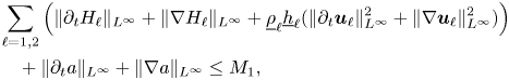
then for any regular solution $\dot {\boldsymbol {U}}=(\dot {\zeta },\dot {\boldsymbol {\phi }}_1,\dot {\boldsymbol {\phi }}_2)^\mathrm {T}$ to the linearized Kakinuma model (6.7) we have

Proof. We deduce from (6.10) that

where we used the fact that $\mathscr {A}_0^\mathrm {mod}$ is a symmetric operator in $L^2$
 and that $\mathscr {A}_1$
 is a skew-symmetric matrix. As for $I_1$
 , we have

Here, as in the proof of lemma 6.1 we have $\sqrt {\underline {\rho }_\ell /\underline {h}_\ell }\theta _\ell (|\boldsymbol {v}|+|\partial _t \boldsymbol {v}|) \lesssim 1$ for $\ell =1,2$
 . In view of the relations $\partial _t\theta _1=-\partial _t\theta _2=\theta _1\theta _2(H_1^{-1}\partial _t H_1 - H_2^{-1}\partial _t H_2)$
 , we have $|\partial _t\theta _\ell | \lesssim \theta _1\theta _2$
 for $\ell =1,2$
 . Therefore, we obtain $|I_1| \lesssim \mathscr {E}(\dot {\boldsymbol {U}})$
 . As for $I_2$
 , by integration by parts we have

By using (2.14), we see that

Therefore, we have $|\boldsymbol {u}| \leq \theta _2|\boldsymbol {u}_1|+\theta _1|\boldsymbol {u}_2| \lesssim 1$ . In view of $|\nabla \theta _\ell | \lesssim \theta _1\theta _2$
 for $\ell =1,2$
 , we have also $|\nabla \boldsymbol {u}| \lesssim 1$
 and $\sqrt {\rho _\ell /\underline {h}_\ell }\theta _l|\nabla \boldsymbol {v}| \lesssim 1$
 for $\ell =1,2$
 . Hence, we obtain $|I_2| \lesssim \mathscr {E}(\dot {\boldsymbol {U}})$
 . Finally, as for $I_3$
 , we have

Summarizing the above estimates we obtain

This together with lemma 6.1 and Gronwall's inequality gives the desired estimate.
6.2 Energy estimates
In this subsection, we will complete the proof of theorem 3.1. The existence and the uniqueness of the solution to the initial value problem for the Kakinuma model (6.1) has already been established in the companion paper [Reference Duchêne and Iguchi14], so that it is sufficient to derive the uniform bound (3.14) of the solution for some time interval $[0,T]$ independent of parameters. The following lemma can be shown in the same way as the proof of [Reference Iguchi19, lemma 4.2].
Lemma 6.3 Let $c,M$ be positive constants and $m$
 an integer such that $m>\frac {n}{2}+1$
 . There exists a positive constant $C$
 such that for any positive parameters $\underline {h}_1, \underline {h}_2, \delta$
 satisfying $\underline {h}_1\delta, \underline {h}_2\delta \leq 1$
 , if $\zeta \in H^{m-1}$
 , $b\in W^{m,\infty }$
 , $H_1=1-\underline {h}_1^{-1}\zeta$
 and $H_2=1+\underline {h}_2^{-1}\zeta -\underline {h}_2^{-1}b$
 satisfy

and if $\boldsymbol {\varphi }_1$ and $\boldsymbol {\varphi }_2$
 satisfy

then for any $k=0,\pm 1,\ldots,\pm (m-1)$ we have

The next lemma gives an energy estimate of the solution to the Kakinuma model (6.1) under appropriate assumptions on the solution. We recall that the mathematical energy function $E_m(t)$ is defined by (5.3).
Lemma 6.4 Let $c,M,M_1,\underline {h}_\mathrm {min}$ be positive constants. There exist two positive constants $C=C(c,M,\underline {h}_\mathrm {min})$
 and $C_1=C_1(c,M,M_1,\underline {h}_\mathrm {min})$
 such that for any positive parameters $\underline {\rho }_1, \underline {\rho }_2, \underline {h}_1, \underline {h}_2, \delta$
 satisfying the natural restrictions (2.14), $\underline {h}_1\delta, \underline {h}_2\delta \leq 1$
 , and the condition ${\underline {h}_\mathrm {min} \leq \underline {h}_1, \underline {h}_2}$
 , if a regular solution $(\zeta,\boldsymbol {\phi }_1,\boldsymbol {\phi }_2)$
 to the Kakinuma model (6.1) with a bottom topography $b$
 satisfies (6.12), $\underline {h}_2^{-1}\left (\|b\|_{W^{m+1,\infty }} + (\underline {h}_2\delta )\|b\|_{W^{m+2,\infty }} \right ) \leq M_1$
 , and $E_m(t) \leq M_1$
 for some time interval $[0,T]$
 , then we have $E_m(t) \leq C\mathrm {e}^{C_1t}E_m(0)$
 for $0\leq t\leq T$
 .
.
Proof. Let $\beta$ be a multi-index such that $1\leq |\beta |\leq m$
 . Applying $\partial ^\beta$
 to the Kakinuma model (6.1), after a tedious but straightforward calculation, we obtain

where $L_1^\mathrm {pr}$ and $L_2^\mathrm {pr}$
 are defined by (6.6), the function $a$
 by (3.9), and

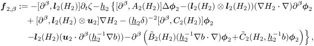
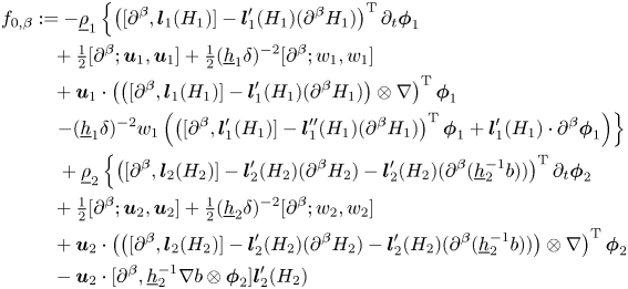
Here, $[\partial ^\beta ;u,v] = \partial ^\beta (uv)-(\partial ^\beta u)v-u(\partial ^\beta v)$ is the symmetric commutator. For vector valued functions, it is defined by $[\partial ^\beta ;\boldsymbol {u},\boldsymbol {v}] = \partial ^\beta (\boldsymbol {u}\cdot \boldsymbol {v}) - (\partial ^\beta \boldsymbol {u})\cdot \boldsymbol {v} - \boldsymbol {u}\cdot (\partial ^\beta \boldsymbol {v})$
 .
.
On the other hand, by lemma 5.2 we have estimate (5.4) for time derivatives of the solution. Particularly, we have

Note that we have also estimate (5.8) for the velocities $(\boldsymbol {u}_\ell,w_\ell )$ $(\ell =1,2)$
 . Moreover, it follows from lemma 6.3 that $\underline {\rho }_\ell \underline {h}_\ell (\underline {h}_\ell \delta )^{-4}\|\boldsymbol {\phi }_\ell '\|_{H^{m-1}}^2 \lesssim E_m$
 for $\ell =1,2$
 . In view of the definition (3.9) of the function $a$
 , it is not difficult to check the estimate $\|a-1\|_{H^m}^2 + \|\partial _t a\|_{H^{m-1}}^2 \lesssim E_m$
 . Therefore, by the Sobolev imbedding theorem we see that all the assumptions in proposition 6.2 are satisfied, so that for the solution $\boldsymbol {U}=(\zeta,\boldsymbol {\phi }_1,\boldsymbol {\phi }_2)^\mathrm {T}$
 we have

where

In view of estimates (5.4), (5.8) and (6.18) together with

for $\ell =1,2$ , we obtain $\mathscr {F}_\beta \lesssim E_m$
 . We note that the multi-index $\beta$
 is assumed to satisfy ${1\leq |\beta |\leq m}$
 . As for the case $\beta =0$
 , in view of $\frac {\mathrm {d}}{\mathrm {d}t}\mathscr {E}(\boldsymbol {U}(t)) \lesssim E_m(t)$
 we infer the inequality $\mathscr {E}({\boldsymbol {U}}(t)) \leq \mathscr {E}({\boldsymbol {U}}(0)) + C_1\int _0^t E_m(\tau ) \mathrm {d}\tau$
 . Summarizing the above estimates we obtain
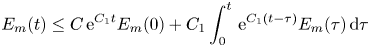
with constants $C=C(c,M,\underline {h}_\mathrm {min})$ and $C_1=C_1(c,M,M_1,\underline {h}_\mathrm {min})$
 . Therefore, Gronwall's inequality gives the desired estimate.
Now, we are ready to prove theorem 3.1. Suppose that the initial data $(\zeta _{(0)},\boldsymbol {\phi }_{1(0)},\boldsymbol {\phi }_{2(0)})$ and the bottom topography $b$
 satisfy (3.10)–(3.13). Let $C_0$
 be a positive constant such that

Such a constant $C_0$ exists as a constant depending on $c_0, M_0, \underline {h}_\mathrm {min}$
 and $m$
 . We will show that the solution $(\zeta,\boldsymbol {\phi }_1,\boldsymbol {\phi }_2)$
 satisfies (3.14), (3.15) and
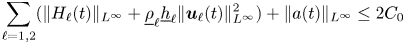
for $0\leq t\leq T$ with a constant $M$
 and a time $T$
 which will be determined below. We note that (3.14) is equivalent to $E_m(t) \leq M$
 . To this end, we assume that the solution satisfies (3.14), (3.15), and (6.19) for $0\leq t\leq T$
 . In the following, the constant depending on $c_0,C_0,\underline {h}_\mathrm {min},m$
 but not on $M$
 is denoted by $C$
 and the constant depending also on $M$
 by $C_1$
 . These constants may change from line to line. Then, it follows from lemma 6.4 that $E_m(t)\leq C\,\text {e}^{C_1t}M_0$
 for $0\leq t\leq T$
 . Therefore, if we chose $M=2CM_0$
 and if $T$
 is so small that $T \leq C_1^{-1}\log 2$
 , then (3.14) holds in fact for $0\leq t\leq T$
 . It remains to show (3.15) and (6.19). As before, we can check
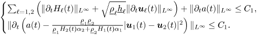
Therefore, if $T$ is so small that $T\leq (2C_1)^{-1}c_0$
 and $T\leq ((2C_0^{1/2}+1)C_1)^{-1}C_0$
 , then the lower bound (3.15) and the upper bound (6.19) hold in fact for $0\leq t\leq T$
 . This completes the proof of theorem 3.1.
7. Approximation of solutions; proof of theorem 3.9
In this section, we prove theorem 3.9, which gives a rigorous justification of the Kakinuma model (2.18) as a higher order shallow water approximation to the full model for interfacial gravity waves (2.17) under the hypothesis of the existence of the solution to the full model with uniform bounds.
7.1 Supplementary estimate for the Dirichlet-to-Neumann map
In this subsection, we give a supplementary estimate to lemma 4.2 for the Dirichlet-to-Neumann map $\Lambda (\zeta,b,\delta )$ defined by (4.6) appearing in the framework of surface waves. We recall the map $\Lambda ^{(N)}(\zeta,b,\delta ) \colon \phi \mapsto \mathcal {L}_0(H,b,\delta )\boldsymbol {\phi }$
 , where $\mathcal {L}_0(H,b,\delta )$
 is defined by (4.3) and $\boldsymbol {\phi }$
 is the unique solution to (4.5). In this section, we omit the dependence of $t$
 in notations.
Lemma 7.1 Let $c, M$ be positive constants and $m, j$
 integers such that $m>\frac {n}{2}+1$
 , $m\geq 2(j+1)$
 and $1\leq j\leq 2N+1$
 . We assume (H1) or (H2). There exists a positive constant $C$
 such that if $\zeta \in H^m$
 , $b\in W^{m+1,\infty }$
 and $H=1+\zeta -b$
 satisfy (4.8), then for any $\phi \in \mathring {H}^{k+2(j+1)}$
 with $0\leq k\leq m-2(j+1)$
 and any $\delta \in (0,1]$
 we have

Proof. This lemma can be proved in a similar way to the proof of lemma 4.2 with a slight modification. For the completeness, we sketch the proof. By the duality $(H^k)^*=H^{-k}$ and the symmetry of the operator $(-\Delta )^{-\frac 12}$
 , it is sufficient to show the estimate

for any $\phi \in \mathring {H}^{k+2(j+1)}$ and any $\psi \in H^{1-k}$
 . We decompose it as

and evaluate the two components of the right-hand side separately.
We recall the definitions (4.1) of the $(N^*+1)$ vector-valued function $\boldsymbol {l}(H)$
 and (4.3) of the operator $\mathcal {L}_i(H,b,\delta )$
 , which acts on $(N^*+1)$
 vector-valued functions. These depend on $N$
 , so that we denote them by $\boldsymbol {l}^{(N)}(H)$
 and $\mathcal {L}_i^{(N)}(H,b,\delta )$
 , respectively, in the following argument. Let $\Phi$
 be the solution to the boundary value problem (4.7) and let $\boldsymbol {\phi }=(\phi _0,\phi _1,\ldots,\phi _{N^*})$
 , $\tilde {\boldsymbol {\phi }}=(\tilde {\phi }_0,\tilde {\phi }_1,\ldots,\tilde {\phi }_{2N^*+2})$
 , and $\boldsymbol {\psi }=(\psi _0,\psi _1,\ldots,\psi _{2N^*+2})$
 be the solutions to the problems


and

respectively. Put

and $\Phi ^\mathrm {res}:=\Phi -\tilde {\Phi }^\mathrm {app}$ . We note that $\tilde {\Phi }^\mathrm {app}$
 is a higher order approximation of the velocity potential $\Phi$
 and that it satisfies the boundary value problem (4.7) approximately in the sense that

where the residual $R$ can be written in the form

Estimates for the residuals $(r_0,r_1,\ldots,r_{2N^*+2})$ and $r_B$
 were given in [Reference Iguchi19, lemmas 6.4 and 6.9]. In fact, we have $\|(r_0,r_1,\ldots,r_{2N^*+2})\|_{H^k}+\|r_B\|_{H^k} \lesssim \delta ^{2j}\|\nabla \phi \|_{H^{k+2j+1}}$
 for $-m\leq k\leq m-2(j+1)$
 and $0\leq j\leq 2N+1$
 .
.
Now, with a slight modification from the strategy in [Reference Iguchi19], we use the identity
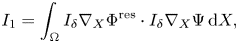
where we denote $\Omega :=\{X=(\boldsymbol {x},z) \,; - 1+b(\boldsymbol {x})< z<\zeta (\boldsymbol {x})\}$ , $I_\delta := \operatorname {diag}(1,\ldots, 1,\delta ^{-1})$
 and $\nabla _X:=(\nabla,\partial _z)=(\partial _1,\ldots,\partial _n,\partial _z)$
 . Indeed, we have on one hand

as a consequence of (4.7), $\Psi (\boldsymbol {x},\zeta (\boldsymbol {x}))=\psi (\boldsymbol {x})$ and Green's identity, and on the other hand
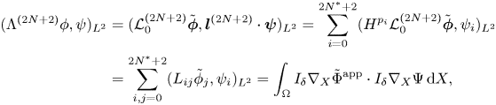
where the last identity follows from expressions (4.2) and (7.1).
To evaluate $I_1$ , it is convenient to transform the water region $\Omega$
 into a simple flat domain $\Omega _0=\mathbf {R}^n\times (-1,0)$
 by using a diffeomorphism which simply stretches the vertical direction $\Theta (\boldsymbol {x},z)=(\boldsymbol {x},\theta (\boldsymbol {x},z)) \colon \Omega _0\to \Omega$
 , where $\theta (\boldsymbol {x},z)=\zeta (\boldsymbol {x}) (z+1)+(1-b(\boldsymbol {x}))z$
 . Put $\tilde {\Phi }^\mathrm {res}=\Phi ^\mathrm {res}\circ \Theta$
 and $\tilde {\Psi }=\Psi \circ \Theta$
 . Then, the above integral is transformed into

where

Therefore, under the restriction $|k|\leq m-1$ and using hypothesis (4.8), we have

where $J=(1-\Delta )^\frac 12$ . Moreover, $\tilde {\Phi }^\mathrm {res}$
 satisfies the boundary value problem
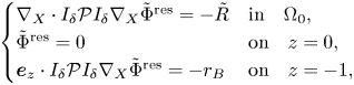
where $\tilde {R} = R\circ \Theta = \sum _{i=0}^{2N^*+2}(z+1)^{p_i}H^{p_i}r_j$ and $\boldsymbol {e}_z=(0,\ldots,0,1)^\mathrm {T}$
 . By applying the standard theory of elliptic partial differential equations to the above problem, for $0\leq k\leq m-1$
 we have

Moreover, in view of $\tilde {\Psi }=\sum _{i=0}^{2N^*+2}(z+1)^{p_i}H^{p_i}\psi _j$ and by lemma 4.1, we have

for $|k|\leq m-1$ . Summarizing the above estimates we have $|I_1| \lesssim \delta ^{2j+1}\|\nabla \phi \|_{H^{k+2j+1}} \|\nabla \psi \|_{H^{-k}}$
 for $0\leq k\leq m-2(j+1)$
 and $0\leq j\leq 2N+1$
 .
.
As for the term $I_2$ , the evaluation is exactly the same as in [Reference Iguchi19]. In fact, the identities

were shown in [Reference Iguchi19, equation (7.7)], where $\boldsymbol {\varphi }:=(\varphi _0,\varphi _1,\ldots,\varphi _{N^*})$ was defined by $\varphi _i:=\phi _i-\tilde {\phi }_i$
 for $i=0,1,\ldots,N^*$
 . Now, we decompose $j=j_1+j_2$
 such that $1\leq j_1\leq N+1$
 and $0\leq j_2\leq N$
 . Then, by [Reference Iguchi19, lemmas 5.2, 5.4, 6.2 and 6.7] we see that

if $\max \{|k|,|k+2j_1-2|,|k+2j_1+1|,|k+2(j_1+j_2)|\} \leq m-1$ and $\max \{|k|,|k+1|,|k+2j_1-1|\}\leq m$
 . These conditions are satisfied under the restriction $-m+1\leq k\leq m-2(j+1)$
 .
.
To summarize, we obtain as desired $|((\Lambda -\Lambda ^{(N)})\phi,\psi )_{L^2}| \lesssim \delta ^{2j}\|\nabla \phi \|_{H^{k+2j+1}} \|\nabla \psi \|_{H^{-k}}$ for $0\leq k\leq m-2(j+1)$
 and $1\leq j\leq 2N+1$
 . The proof is complete.
This lemma and the scaling relations (4.15) imply immediately the following lemma.
Lemma 7.2 Let $c, M$ be positive constants and $m,j$
 integers such that $m>\frac {n}{2}+1$
 , $m\geq 2(j+1)$
 and $1\leq j\leq 2N+1$
 . We assume (H1) or (H2). There exists a positive constant $C$
 such that for any positive parameters $\underline {h}_1, \underline {h}_2, \delta$
 satisfying $\underline {h}_1\delta, \underline {h}_2\delta \leq 1$
 , if $\zeta \in H^m$
 , $b\in W^{m+1,\infty }$
 , $H_1 = 1 - \underline {h}_1^{-1}\zeta$
 and $H_2 = 1 + \underline {h}_2^{-1}\zeta - \underline {h}_2^{-1}b$
 satisfy (4.14), then for any $\phi _1,\phi _2 \in \mathring {H}^{k+2(j+1)}$
 with $0\leq k\leq m-2(j+1)$
 we have

We recall also the estimate for the Dirichlet-to-Neumann map $\Lambda (\zeta,b,\delta )$ itself. The following lemma is now standard. For sharper estimates, we refer to Iguchi [Reference Iguchi17] and Lannes [Reference Lannes29].
Lemma 7.3 Let $c, M$ be positive constants $m$
 an integer such that $m>\frac {n}{2}+2$
 . There exists a positive constant $C$
 such that if $\zeta \in H^m$
 , $b\in W^{m,\infty }$
 and $H=1+\zeta -b$
 satisfy (4.4), then for any $\phi \in \mathring {H}^{k+1}$
 with $|k|\leq m-1$
 and any $\delta \in (0,1]$
 we have $\|\Lambda (\zeta,b,\delta )\phi \|_{H^{k-1}} \leq C \|\nabla \phi \|_{H^k}$
 .
.
This lemma and the scaling relations (4.15) imply immediately the following lemma.
Lemma 7.4 Let $c, M$ be positive constants and $m$
 an integer such that $m>\frac {n}{2}+2$
 . There exists a positive constant $C$
 such that for any positive parameters $\underline {h}_1, \underline {h}_2, \delta$
 satisfying $\underline {h}_1\delta, \underline {h}_2\delta \leq 1$
 , if $\zeta \in H^m$
 , $b\in W^{m,\infty }$
 , $H_1 = 1 - \underline {h}_1^{-1}\zeta$
 and $H_2 = 1 + \underline {h}_2^{-1}\zeta - \underline {h}_2^{-1}b$
 satisfy (4.11), then for any $\phi _1,\phi _2 \in \mathring {H}^{k+1}$
 with $|k|\leq m-1$
 we have

7.2 Consistency of the Kakinuma model revisited
As we mentioned in remark 3.8, the approximate solution to the Kakinuma model (2.18) made from the solution $(\zeta,\phi _1,\phi _2)$ to the full model can be constructed as a solution to (3.21), that is,

in place of (3.19), that is,

To show this fact, we need to guarantee that the difference between these two solutions is of order $O((\underline {h}_1\delta )^{4N+2}+(\underline {h}_2\delta )^{4N+2})$ . The following lemma gives such an estimate.
Lemma 7.5 Let $c, M$ be positive constants and $m$
 an integer such that $m>\frac {n}{2}+1$
 and ${m\geq 4(N+1)}$
 . We assume (H1) or (H2). There exists a positive constant $C$
 such that for any positive parameters $\underline {\rho }_1, \underline {\rho }_2, \underline {h}_1, \underline {h}_2, \delta$
 satisfying $\underline {h}_1\delta, \underline {h}_2\delta \leq 1$
 , if $\zeta \in H^m$
 , $b\in W^{m+1,\infty }$
 , $H_1 = 1 - \underline {h}_1^{-1}\zeta$
 and $H_2 = 1 + \underline {h}_2^{-1}\zeta - \underline {h}_2^{-1}b$
 satisfy (4.14), then for any $\phi _1,\phi _2 \in \mathring {H}^{k+4(N+1)}$
 with $0\leq k\leq m-4(N+1)$
 satisfying the compatibility condition $\Lambda _1(\zeta,\delta,\underline {h}_1)\phi _1+\Lambda _2(\zeta,b,\delta,\underline {h}_2)\phi _2=0$
 the solution $(\boldsymbol {\phi }_1,\boldsymbol {\phi }_2)$
 to (7.3) and the solution $(\tilde {\boldsymbol {\phi }}_1,\tilde {\boldsymbol {\phi }}_2)$
 to (7.2) satisfy

Proof. For simplicity, we write $\mathcal {L}_{1,i}=\mathcal {L}_{1,i}(H_1,\delta,\underline {h}_1)$ , $\boldsymbol {l}_1=\boldsymbol {l}_1(H_1)$
 , and so on. We recall that $\Lambda _1^{(N)}\colon \phi _1 \mapsto \mathcal {L}_{1,0}\boldsymbol {\phi }_1$
 and $\Lambda _2^{(N)}\colon \phi _2 \mapsto \mathcal {L}_{2,0}\boldsymbol {\phi }_2$
 . Notice that $\tilde {\boldsymbol {\phi }}_\ell -\boldsymbol {\phi }_\ell$
 for $\ell =1,2$
 satisfy

Since the right-hand side of the third equation can be written as $\nabla \cdot \boldsymbol {f}_3$ with
with

by lemmas 5.1 and 7.2 we obtain

Moreover, it follows from lemma 6.3 that

for $\ell =1,2$ . This completes the proof.
The following proposition gives another version of theorem 3.6 for the consistency of the Kakinuma model.
Proposition 7.6 Let $c, M$ be positive constants and $m$
 an integer such that $m \geq 4N+4$
 and $m>\frac {n}{2}+2$
 . We assume (H1) or (H2). There exists a positive constant $C$
 such that for any positive parameters $\underline {\rho }_1, \underline {\rho }_2, \underline {h}_1, \underline {h}_2, \delta$
 satisfying $\underline {h}_1\delta, \underline {h}_2\delta \leq 1$
 , and for any solution $(\zeta,\phi _1,\phi _2)$
 to the full model for interfacial gravity waves (2.17) on a time interval $[0,T]$
 satisfying (3.18), if we define $H_1$
 and $H_2$
 as in (2.19) and $(\tilde {\boldsymbol {\phi }}_1,\tilde {\boldsymbol {\phi }}_2)$
 as a solution to (7.2), then $(\zeta,\tilde {\boldsymbol {\phi }}_1,\tilde {\boldsymbol {\phi }}_2)$
 satisfy approximately the Kakinuma model as

where $\tilde {\boldsymbol {u}}_1, \tilde {\boldsymbol {u}}_2, \tilde {w}_1, \tilde {w}_2$ are defined by (3.4) with $(\boldsymbol {\phi }_1,\boldsymbol {\phi }_2)$
 replaced by $(\tilde {\boldsymbol {\phi }}_1,\tilde {\boldsymbol {\phi }}_2)$
 , and the errors $(\boldsymbol {\mathfrak {r}}_1,\boldsymbol {\mathfrak {r}}_2,\mathfrak {r}_0)$
 satisfy

for $t\in [0,T]$ .
.
Proof. Let $\boldsymbol {\phi }_1$ and $\boldsymbol {\phi }_2$
 be the unique solutions to (7.3), and $(\tilde {\boldsymbol {\mathfrak {r}}}_1,\tilde {\boldsymbol {\mathfrak {r}}}_2,\tilde {\mathfrak {r}}_0)$
 the errors in theorem 3.6. Then, the errors $(\boldsymbol {\mathfrak {r}}_1,\boldsymbol {\mathfrak {r}}_2,\mathfrak {r}_0)$
 in the proposition can be written as

Therefore, we have

for $-m\leq k\leq m-1$ and $\ell =1,2$
 . Applying this estimate with $k=m-(4N+5)$
 and the estimate in lemma 7.5 with $k=m-4(N+1)$
 and using the result in theorem 3.6, we obtain the first estimate in (7.5). Since $m-2>\frac {n}{2}$
 , we have

for $|k|\leq m-2$ . Here, it follows from lemmas 4.4, 5.1 and 7.5 that


and

for $0\leq k\leq m-4(N+1)$ . Moreover, it follows from lemma 7.4 that $\|\partial _t\zeta \|_{H^{m-2}} = \|\Lambda _\ell \phi _\ell \|_{H^{m-2}}\lesssim \underline {h}_\ell \|\nabla \phi _\ell \|_{H^{m-1}}$
 for $\ell =1,2$
 . Summarizing the above estimates and using the result in theorem 3.6, we easily obtain the second estimate in (7.5). The proof is complete.
7.3 Completion of the proof of theorem 3.9
Now we are ready to prove theorem 3.9. Let $(\zeta ^{{\rm IW}},\phi _1^{{\rm IW}},\phi _2^{{\rm IW}})$ be the solution to the full model for interfacial gravity waves (2.17) with uniform bound stated in the theorem, and define ${\phi ^{{\rm IW}}:=\underline {\rho }_2\phi _2^{{\rm IW}}-\underline {\rho }_1\phi _1^{{\rm IW}}}$
 , which is a canonical variable of the full model. We first ensure a uniform bound on the time derivative of the canonical variables $(\zeta ^{{\rm IW}},\phi ^{{\rm IW}})$
 . It follows from the first and the second equations in (2.17) that $\partial _t\zeta ^{{\rm IW}}=-\Lambda _1^{{\rm IW}}\phi _1^{{\rm IW}} =\Lambda _2^{{\rm IW}}\phi _2^{{\rm IW}}$
 , where $\Lambda _1^{{\rm IW}}=\Lambda _1(\zeta ^{{\rm IW}},\delta,\underline {h}_1)$
 and $\Lambda _2^{{\rm IW}}=\Lambda _2(\zeta ^{{\rm IW}},b,\delta,\underline {h}_2)$
 . Similar notations will be used in the following without any comment. Therefore, by lemma 7.4 we have
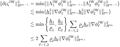
where we used (2.15). It follows from the third equation in (2.17) that
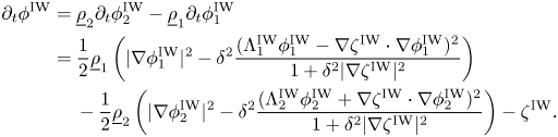
Here, we note that in view of the conditions $\underline {h}_1\delta, \underline {h}_2\delta \leq 1$ and $\underline {h}_1^{-1}, \underline {h}_2^{-1}\lesssim 1$
 we have $\delta \lesssim 1$
 . Therefore, by lemma 7.4 we have
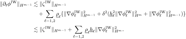
Hence, we obtain $\|\partial _t\zeta ^{{\rm IW}}\|_{H^{m-1}}+\|\partial _t\phi ^{{\rm IW}}\|_{H^{m-1}} \lesssim 1$ .
.
Let $(\tilde {\boldsymbol {\phi }}_1^{{\rm IW}},\tilde {\boldsymbol {\phi }}_2^{{\rm IW}})$ be the solution to (7.2) with $(\zeta,\phi )=(\zeta ^{{\rm IW}},\phi ^{{\rm IW}})$
 . Then, proposition 7.6 states that $(\zeta ^{{\rm IW}},\tilde {\boldsymbol {\phi }}_1^{{\rm IW}},\tilde {\boldsymbol {\phi }}_2^{{\rm IW}})$
 satisfy approximately the Kakinuma model as (7.4) and the errors $(\boldsymbol {\mathfrak {r}}_1,\boldsymbol {\mathfrak {r}}_2,\mathfrak {r}_0)$
 satisfy (7.5). Moreover, it follows from lemma 5.1 that

which yields

where $\tilde {\boldsymbol {u}}_1^{{\rm IW}}, \tilde {\boldsymbol {u}}_2^{{\rm IW}}, \tilde {w}_1^{{\rm IW}}, \tilde {w}_2^{{\rm IW}}$ are defined by (3.4) with $(\boldsymbol {\phi }_1,\boldsymbol {\phi }_2)$
 replaced by $(\tilde {\boldsymbol {\phi }}_1^{{\rm IW}},\tilde {\boldsymbol {\phi }}_2^{{\rm IW}})$
 , and we used lemma 6.3. We proceed to evaluate $(\partial _t\tilde {\boldsymbol {\phi }}_1^{{\rm IW}},\partial _t\tilde {\boldsymbol {\phi }}_2^{{\rm IW}})$
 . To this end, we derive equations for these time derivatives by differentiating (7.2) with respect to $t$
 . The procedure is almost the same as in the proof of lemma 5.2. The only difference is the last equation in (5.5), especially, the expression of $f_4$
 . In this case, $f_4$
 has the form

so that $\|f_4\|_{H^{m-1}} \lesssim 1$ . Therefore, we obtain
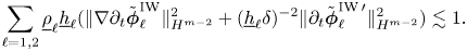
Let $(\zeta ^{{\rm K}},\boldsymbol {\phi }_1^{{\rm K}},\boldsymbol {\phi }_2^{{\rm K}})$ be the solution to the initial value problem for the Kakinuma model (2.18)–(2.20) stated in the theorem, whose unique existence is guaranteed by theorem 3.1 and proposition 3.4. Note also that the solution satisfies the uniform bound (3.14) together with the stability and non-cavitation conditions (3.15). It follows from lemma 6.3 that $\underline {\rho }_\ell \underline {h}_\ell (\underline {h}_\ell \delta )^{-4} \|\boldsymbol {\phi }_\ell ^{{\rm K} \, \prime }\|_{H^{m-1}}^2 \lesssim 1$
 for $\ell =1,2$
 . Moreover, the time derivatives $(\partial _t\zeta ^{{\rm K}},\partial _t\boldsymbol {\phi }_1^{{\rm K}},\partial _t\boldsymbol {\phi }_2^{{\rm K}})$
 satisfy (5.4) and $(\boldsymbol {u}_\ell ^{{\rm K}},w_\ell ^{{\rm K}})$ $(\ell =1,2)$
 , which are defined by (3.4) with $(\boldsymbol {\phi }_1,\boldsymbol {\phi }_2)$
 replaced by $({\boldsymbol {\phi }}_1^{{\rm K}},{\boldsymbol {\phi }}_2^{{\rm K}})$
 , satisfy (5.8). Putting

we will show that $(\zeta ^\mathrm {res},\boldsymbol {\phi }_1^\mathrm {res},\boldsymbol {\phi }_2^\mathrm {res})$ can be estimated by the errors $(\boldsymbol {\mathfrak {r}}_1,\boldsymbol {\mathfrak {r}}_2,\mathfrak {r}_0)$
 . To this end, we are going to evaluate

for an appropriate integer $k$ by making use of energy estimates similar to the ones obtained in § 5 and 6 for the proof of the well-posedness of the initial value problem for the Kakinuma model (2.18)–(2.20). Here, we note that $E_k^\mathrm {res}(0)=0$
 .
.
As in the case of the energy estimate for the Kakinuma model, we first need to evaluate times derivatives $(\partial _t\zeta ^\mathrm {res},\partial _t\boldsymbol {\phi }_1^\mathrm {res},\partial _t\boldsymbol {\phi }_2^\mathrm {res})$ in terms of $E_k^\mathrm {res}$
 . By taking difference between the first components of the first two equations in (3.5) and (7.4), $\partial _t\zeta ^\mathrm {res}$
 can be written in two ways as

where $\mathcal {L}_{1,0}^{{\rm K}}=\mathcal {L}_{1,0}(H_1^{{\rm K}},\delta,\underline {h}_1)$ , $H_1^{{\rm K}}=1-\underline {h}_1^{-1}\zeta ^{{\rm K}}$
 and similar simplifications are used, and $\mathfrak {r}_{\ell,0}$
 is the $0$
 th component of the error $\boldsymbol {\mathfrak {r}}_\ell$
 for $\ell =1,2$
 . Therefore, we have
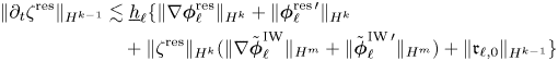
for $\ell =1,2$ and $|k|\leq m$
 . Hence, by the technique used in the proof of lemma 5.2 we obtain

for $|k|\leq m$ . We proceed to evaluate $(\partial _t\boldsymbol {\phi }_1^\mathrm {res},\partial _t\boldsymbol {\phi }_2^\mathrm {res})$
 . We recall that $(\partial _t\boldsymbol {\phi }_1^{{\rm K}},\partial _t\boldsymbol {\phi }_2^{{\rm K}})$
 satisfy (5.5) with $(\zeta,\boldsymbol {\phi }_1,\boldsymbol {\phi }_2)=(\zeta ^{{\rm K}},\boldsymbol {\phi }_1^{{\rm K}},\boldsymbol {\phi }_2^{{\rm K}})$
 and note that, differentiating the first three equations of (7.2) with respect to $t$
 and using the last equation in (7.4), $(\partial _t\tilde {\boldsymbol {\phi }}_1^{{\rm IW}},\partial _t\tilde {\boldsymbol {\phi }}_2^{{\rm IW}})$
 also satisfy (5.5) with $(\zeta,\boldsymbol {\phi }_1,\boldsymbol {\phi }_2) =(\zeta ^{{\rm IW}},\tilde {\boldsymbol {\phi }}_1^{{\rm IW}},\tilde {\boldsymbol {\phi }}_2^{{\rm IW}})$
 and $f_4$
 added with the error term $-\mathfrak {r}_0$
 . By taking the difference between these equations, we have therefore

where

Here, $f_{1,i}^{{\rm K}}$ , $f_{2,i}^{{\rm K}}$
 , $\boldsymbol {f}_3^{{\rm K}}$
 , $f_4^{{\rm K}}$
 (respectively $\tilde {f}_{1,i}^{{\rm IW}}$
 , $\tilde {f}_{2,i}^{{\rm IW}}$
 , $\tilde {\boldsymbol {f}}_3^{{\rm IW}}$
 , $\tilde {f}_4^{{\rm IW}}$
 ) are those in (5.6) with $(\zeta,\boldsymbol {\phi }_1,\boldsymbol {\phi }_2) =(\zeta ^{{\rm K}},\boldsymbol {\phi }_1^{{\rm K}},\boldsymbol {\phi }_2^{{\rm K}})$
 (respectively $(\zeta,\boldsymbol {\phi }_1,\boldsymbol {\phi }_2) =(\zeta ^{{\rm IW}},\tilde {\boldsymbol {\phi }}_1^{{\rm IW}},\tilde {\boldsymbol {\phi }}_2^{{\rm IW}})$
 ), $\boldsymbol {a}_{\ell,0}^{{\rm K}}=\boldsymbol {a}_{\ell,0}(H_\ell ^{{\rm K}})$
 and $\boldsymbol {b}_{2,0}^{{\rm K}}=\boldsymbol {b}_{2,0}(H_2^{{\rm K}})$
 , where $\boldsymbol {a}_{\ell,0}(H_\ell )$
 and $\boldsymbol {b}_{2,0}(H_2)$
 are the $0$
 th columns of the matrixes $A_\ell (H_\ell )$
 and $B_2(H_2)$
 defined by (6.2) and (6.4), respectively, and so on. Note the relations $\mathcal {L}_{1,0}\boldsymbol {\phi }_1=-\nabla \cdot ((\boldsymbol {a}_{1,0}\otimes \nabla )^\mathrm {T}\boldsymbol {\phi }_1)$
 and $\mathcal {L}_{2,0}\boldsymbol {\phi }_2=-\nabla \cdot ((\boldsymbol {a}_{2,0}\otimes \nabla )^\mathrm {T}\boldsymbol {\phi }_2 -(\boldsymbol {b}_{2,0}\cdot \boldsymbol {\phi }_2)\underline {h}_2^{-1}\nabla b)$
 . Therefore, by lemma 5.1 we have, for $1\leq k\leq m+1$
 ,
,
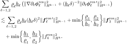
We will evaluate each term in the right-hand side. For $1\leq k\leq m-1$ , we see that

for $\ell =1,2$ ,
,

and
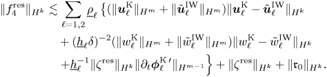
Moreover, for any $0\leq k\leq m$ we have also

Summarizing the above estimates and using $\underline {h}_1^{-1}, \underline {h}_2^{-1}\lesssim 1$ we obtain, for $1\leq k\leq m-1$
 ,
,
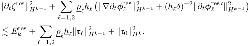
We need also to evaluate $\underline {\rho }_\ell \underline {h}_\ell (\underline {h}_\ell \delta )^{-4} \|\boldsymbol {\phi }_\ell ^{\mathrm {res} \, \prime }\|_{H^{k-1}}^2$ for $\ell =1,2$
 in terms of $E_k^\mathrm {res}$
 . In view of

Lemma 6.3 yields $(\underline {h}_\ell \delta )^{-2} \|\boldsymbol {\phi }_\ell ^{\mathrm {res} \, \prime }\|_{H^{k-1}}\lesssim \|\nabla \boldsymbol {\phi }_\ell ^\mathrm {res}\|_{H^k} + \|\boldsymbol {\phi }_\ell ^{\mathrm {res} \, \prime } \|_{H^{k}} + \|\boldsymbol {h}_\ell ^{\mathrm {res} \, \prime }\|_{H^{k-1}}$ and we have $\|\boldsymbol {h}_\ell ^{\mathrm {res} \, \prime }\|_{H^{k-1}} \lesssim (\|\nabla \boldsymbol {\phi }_\ell ^{{\rm K}}\|_{H^m} + \|\boldsymbol {\phi }_\ell ^{{\rm K} \, \prime }\|_{H^m} + (\underline {h}_\ell \delta )^{-2}\|\boldsymbol {\phi }_\ell ^{{\rm K} \, \prime }\|_{H^{m-1}}) \|\zeta ^\mathrm {res}\|_{H^k}$
 for $1\leq k\leq m$
 . Therefore, for $1\leq k\leq m$
 we obtain

Now, by deriving equations for spatial derivatives of $(\zeta ^\mathrm {res},\boldsymbol {\phi }_1^\mathrm {res},\boldsymbol {\phi }_2^\mathrm {res})$ and applying the energy estimate obtained in § 6.1 we will evaluate $E_{k}^\mathrm {res}$
 . Let $\beta$
 be a multi-index such that $1\leq |\beta |\leq k$
 . Applying $\partial ^\beta$
 to the Kakinuma model (3.5) for $(\zeta ^{{\rm K}},\boldsymbol {\phi }_1^{{\rm K}},\boldsymbol {\phi }_2^{{\rm K}})$
 and to (7.4) for $(\zeta ^{{\rm IW}},\tilde {\boldsymbol {\phi }}_1^{{\rm IW}},\tilde {\boldsymbol {\phi }}_2^{{\rm IW}})$
 and taking the difference between the resulting equations, we obtain

where
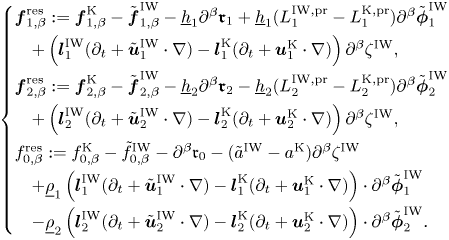
Here, $\boldsymbol {f}_{1,\beta }^{{\rm K}}$ , $\boldsymbol {f}_{2,\beta }^{{\rm K}}$
 and $f_{0,\beta }^{{\rm K}}$
 are those in (6.15)–(6.17) with $(\zeta,\boldsymbol {\phi }_1,\boldsymbol {\phi }_2) =(\zeta ^{{\rm K}},\boldsymbol {\phi }_1^{{\rm K}},\boldsymbol {\phi }_2^{{\rm K}})$
 , and so on. As we saw, all the assumptions in proposition 6.2 are satisfied, so that we have

where $\boldsymbol {U}^\mathrm {res}:=(\zeta ^\mathrm {res},\boldsymbol {\phi }_1^\mathrm {res},\boldsymbol {\phi }_2^\mathrm {res})^\mathrm {T}$ , $\mathscr {E}$
 is defined in (6.11), and

In view of $\|(\zeta ^{{\rm IW}},\zeta ^{{\rm K}})\|_{H^m} \lesssim 1$ , straightforward calculations yield

for $\ell =1,2$ and $\frac {n}{2}< k\leq m-1$
 . As for $f_{0,\beta }^\mathrm {res}$
 , we note the relation
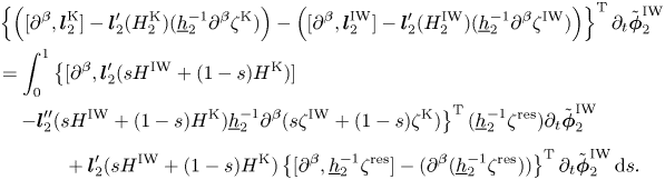
Therefore, straightforward calculations yield
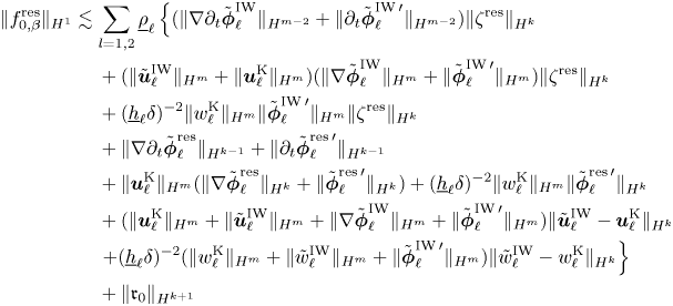
for $\frac {n}{2}< k\leq m-2$ . In view of the above estimates and (7.6)–(7.8) we obtain $\mathscr {F}_\beta ^\mathrm {res} \lesssim E_k^\mathrm {res} + \mathfrak {R}_k$
 with $\mathfrak {R}_k := \|\mathfrak {r}_0\|_{H^{k+1}}^2 + \sum _{l=1,2}\underline {\rho }_\ell \underline {h}_\ell \|\boldsymbol {\mathfrak {r}}_\ell \|_{H^k}^2$
 . We note that the multi-index $\beta$
 is assumed to satisfy $1\leq |\beta |\leq k$
 . As for the case $\beta =0$
 , we have $\frac {\mathrm {d}}{\mathrm {d}t}E_0^\mathrm {res}(t) \lesssim E_k^\mathrm {res}(t)$
 , hence ${E_0^\mathrm {res}(t) \lesssim \int _0^tE_k^\mathrm {res}(\tau )\mathrm {d}\tau }$
 . Summarizing the above estimates we obtain $E_k^\mathrm {res}(t) \lesssim \int _0^t(E_k^\mathrm {res}(\tau )+\mathfrak {R}_k(\tau ))\,\mathrm {d}\tau$
 for $\frac {n}{2}< k\leq m-2$
 . Putting ${k=m-4(N+1)}$
 and applying Gronwall's inequality and (7.5) in proposition 7.6 we obtain $E_{m-4(N+1)}^\mathrm {res}(t) \lesssim (\underline {h}_1\delta )^{4N+2}+(\underline {h}_2\delta )^{4N+2}$
 for $0\leq t\leq \min \{T,T^{{\rm IW}}\}$
 .
.
It remains to evaluate $\phi _\ell ^{{\rm IW}}-\phi _\ell ^{{\rm K}}$ for $\ell =1,2$
 . Let $(\boldsymbol {\phi }_1^{{\rm IW}},\boldsymbol {\phi }_2^{{\rm IW}})$
 be the solution to (3.19) with $(\zeta,\phi _1,\phi _2)=(\zeta ^{{\rm IW}},\phi _1^{{\rm IW}},\phi _2^{{\rm IW}})$
 . Then, we have $\phi _\ell ^{{\rm K}}-\phi _\ell ^{{\rm IW}} = \boldsymbol {l}_\ell ^{{\rm K}}\cdot \boldsymbol {\phi }_\ell ^\mathrm {res} + (\boldsymbol {l}_\ell ^{{\rm K}}-\boldsymbol {l}_\ell ^{{\rm IW}})\cdot \tilde {\boldsymbol {\phi }}_\ell ^{{\rm IW}} + \boldsymbol {l}_\ell ^{{\rm IW}}\cdot (\tilde {\boldsymbol {\phi }}_\ell ^{{\rm IW}}-\boldsymbol {\phi }_\ell ^{{\rm IW}}),$
 so that for any $0\leq k\leq m-1$
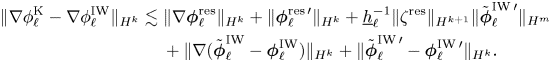
Therefore, the previous result together with lemma 7.5 implies

This completes the proof of theorem 3.9.
8. Approximation of Hamiltonians; proof of theorem 3.10
As was shown in the companion paper [Reference Duchêne and Iguchi14, theorem 8.4], the Kakinuma model (2.18) enjoys a Hamiltonian structure analogous to the one exhibited on the full model for interfacial gravity waves by Benjamin and Bridges in [Reference Benjamin and Bridges3]. In this section, we will prove theorem 3.10, which states that the Hamiltonian $\mathscr {H}^{{\rm K}}(\zeta,\phi )$ of the Kakinuma model defined in (2.25) approximates the Hamiltonian $\mathscr {H}^{{\rm IW}}(\zeta,\phi )$
 of the full model defined in (2.22) with an error of order $O((\underline {h}_1\delta )^{4N+2}+(\underline {h}_2\delta )^{4N+2})$
 .
.
8.1 Preliminary elliptic estimates
We consider the following transmission problem
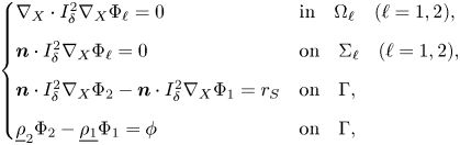
where the rigid-lid $\Sigma _1$ of the upper layer $\Omega _1$
 , the bottom $\Sigma _2$
 of the lower layer $\Omega _2$
 and the interface $\Gamma$
 are defined by $z=\underline {h}_1$
 , $z=-\underline {h}_2+b(\boldsymbol {x})$
 and $z=\zeta (\boldsymbol {x})$
 , respectively, $I_\delta :=\operatorname {diag}(1,\ldots,1,\delta ^{-1})$
 , $\nabla _X:=(\nabla,\partial _z)^\mathrm {T}=(\partial _1,\ldots,\partial _n,\partial _z)$
 and $\boldsymbol {n}$
 is an upward normal vector, specifically, $\boldsymbol {n}=\boldsymbol {e}_z$
 on $\Sigma _1$
 , $\boldsymbol {n}=(-\nabla b, 1)^\mathrm {T}$
 on $\Sigma _2$
 and $\boldsymbol {n}=(-\zeta,1)^\mathrm {T}$
 on $\Gamma$
 .
.
Lemma 8.1 Let $c,M$ be positive constants. There exists a positive constant $C$
 such that for any positive parameters $\underline {\rho }_1, \underline {\rho }_2, \underline {h}_1, \underline {h}_2, \delta$
 satisfying $\underline {h}_1\delta, \underline {h}_2\delta \leq 1$
 , if $\zeta,b \in W^{1,\infty }$
 , $H_1 = 1 - \underline {h}_1^{-1}\zeta$
 and $H_2 = 1 + \underline {h}_2^{-1}\zeta - \underline {h}_2^{-1}b$
 satisfy

then for any $(r_S,\phi )$ satisfying $\nabla \phi \in H^{-\frac 12}$
 and $(-\Delta )^{-\frac 12}r_S\in H^\frac 12$
 there exists a solution $(\Phi _1,\Phi _2)$
 to transmission problem (8.1). The solution is unique up to an additive constant of the form $(\underline {\rho }_2\mathcal {C},\underline {\rho }_1\mathcal {C})$
 and satisfies

where $\Lambda _{1,0}=\Lambda _1(0,\delta,\underline {h}_1)$ and $\Lambda _{2,0}=\Lambda _2(0,0,\delta,\underline {h}_2)$
 are Dirichlet-to-Neumann maps in the case $\zeta (\boldsymbol {x})\equiv b(\boldsymbol {x}) \equiv 0$
 . Particularly, if we further impose $\phi \in \mathring {H}^1$
 , $(-\Delta )^{-\frac 12}r_S\in H^1$
 , the natural restrictions (2.14), and $\underline {h}_\mathrm {min} \leq \underline {h}_1,\underline {h}_2$
 with a positive constant $\underline {h}_\mathrm {min}$
 , then we have

where the constant $C$ depends also on $\underline {h}_\mathrm {min}$
 .
.
Proof. The existence and the uniqueness of the solution is standard, so that we focus on deriving the uniform estimate of the solution. To this end, it is convenient to transform the water regions $\Omega _1$ and $\Omega _2$
 into simple domains $\Omega _{1,0}=\mathbf {R}^n\times (0,\underline {h}_1)$
 and $\Omega _{2,0}=\mathbf {R}^n\times (-\underline {h}_2,0)$
 by using diffeomorphisms $\Theta _\ell (\boldsymbol {x},z)=(\boldsymbol {x},\theta _\ell (\boldsymbol {x},z)) \colon \Omega _{\ell,0}\to \Omega _\ell$ $(\ell =1,2)$
 , respectively, where $\theta _1(\boldsymbol {x},z)=(1-\underline {h}_1^{-1}\zeta (\boldsymbol {x}))z+\zeta (\boldsymbol {x})$
 and $\theta _2(\boldsymbol {x},z)=(1+\underline {h}_2^{-1}(\zeta (\boldsymbol {x})-b(\boldsymbol {x})))z+\zeta (\boldsymbol {x})$
 . Put $\tilde {\Phi }_\ell =\Phi _\ell \circ \Theta _\ell$ $(\ell =1,2)$
 . Then, transmission problem (8.1) is transformed into

where $\Sigma _{1,0}$ , $\Sigma _{2,0}$
 and $\Gamma _0$
 are represented as $z=\underline {h}_1$
 , $z=-\underline {h}_2$
 and $z=0$
 , respectively, and

We note that $\|I_\delta \nabla _X\Phi _\ell \|_{L^2(\Omega _\ell )} \simeq \|I_\delta \nabla _X\tilde {\Phi }_\ell \|_{L^2(\Omega _{\ell,0})}$ $(\ell =1,2)$
 . Let $(\Psi _1,\Psi _2)$
 be a solution to the transmission problem
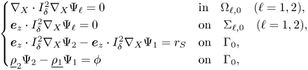
and put $\Phi _\ell ^\mathrm {res}=\tilde {\Phi }_\ell -\Psi _\ell$ $(\ell =1,2)$
 . Then, we can decompose

for $\ell =1,2$ and $\underline {\rho }_1\Phi _1^\mathrm {res}= \underline {\rho }_2\Phi _2^\mathrm {res}$
 on $z=0$
 . Therefore, denoting the unit outward normal vector to $\partial \Omega _{\ell,0}$
 by $N_\ell$ $(\ell =1,2)$
 we have

so that we obtain

Similarly, in view of the decomposition

for $\ell =1,2$ , we obtain

It follows from these two identities that

which yields the equivalence

Therefore, it is sufficient to evaluate the right-hand side of the above equation. In other words, the evaluation is reduced to the simple case $\zeta (\boldsymbol {x})\equiv b(\boldsymbol {x})\equiv 0$ .
.
Putting $\psi _\ell = \Psi _\ell |_{z=0}$ $(\ell =1,2)$
 , we see that

and that

Particularly, we have

Therefore,

Hence, by the linearity of the problem we obtain (8.2).
Finally, in order to show (8.3) it is sufficient to evaluate the symbols of the Fourier multipliers $(\underline {\rho }_1\Lambda _{2,0}+\underline {\rho }_2\Lambda _{1,0})^{-1}\Lambda _{1,0}\Lambda _{2,0}$ and $\underline {\rho }_1\underline {\rho }_2(\underline {\rho }_1\Lambda _{2,0}+\underline {\rho }_2\Lambda _{1,0})^{-1}$
 . We recall that the symbol of the Dirichlet-to-Neumann map $\Lambda _{\ell,0}$
 is given by $\sigma (\Lambda _{\ell,0})=\delta ^{-1}|\boldsymbol {\xi }|\tanh (\underline {h}_\ell \delta |\boldsymbol {\xi }|)$
 for $\ell =1,2$
 . In view of $0\leq \tanh \xi \leq \xi$
 for $\xi \geq 0$
 , we have

where we used (2.15). In view of $\tanh \xi \simeq (1+\xi )^{-1}\xi$ for $\xi \geq 0$
 and relation (2.14), we have

where we used $1\lesssim \underline {h}_1,\underline {h}_2$ . These estimates imply (8.3). The proof is complete.
8.2 Completion of the proof of theorem 3.10
Now we are ready to prove theorem 3.10. We recall the definitions (3.3) of $\boldsymbol {l}_1(H_1)$ , $\boldsymbol {l}_2(H_2)$
 and (3.6) of the operators $\mathcal {L}_{1,i}(H_1,\delta,\underline {h}_1)$
 and $\mathcal {L}_{2,i}(H_2,b,\delta,\underline {h}_2)$
 . These depend on $N$
 , so that we denote them by $\boldsymbol {l}_1^{(N)}(H_1)$
 , $\boldsymbol {l}_2^{(N)}(H_2)$
 and $\mathcal {L}_{1,i}^{(N)}(H_1,\delta,\underline {h}_1)$
 and $\mathcal {L}_{2,i}^{(N)}(H_2,b,\delta,\underline {h}_2)$
 , respectively, in the following argument. For given $(\zeta,\phi )$
 , let $\Phi$
 be the solution to transmission problem (8.1) with $r_S=0$
 and let $(\boldsymbol {\phi }_1,\boldsymbol {\phi }_2)$
 and $(\tilde {\boldsymbol {\phi }}_1,\tilde {\boldsymbol {\phi }}_2)$
 be the solutions to the problems

and
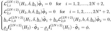
respectively, and define $(\Phi _1^\mathrm {app},\Phi _2^\mathrm {app})$ and $(\tilde {\Phi }_1^\mathrm {app},\tilde {\Phi }_2^\mathrm {app})$
 by (2.24) and
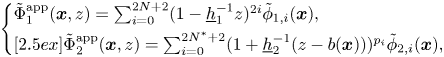
respectively. Then, by the definitions of the Hamiltonian functionals $\mathscr {H}^{{\rm IW}}(\zeta,\phi )$ and $\mathscr {H}^{{\rm K}}(\zeta,\phi )$
 given in § 2.3, we have

We will evaluate $I_1$ and $I_2$
 , separately.
In order to evaluate $I_1$ , we put $\Phi _\ell ^\mathrm {res}=\Phi _\ell -\tilde {\Phi }_\ell ^\mathrm {app}$ $(\ell =1,2)$
 , so that
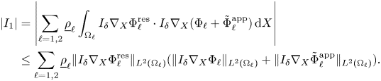
It follows from lemma 8.1 that $\sum _{\ell =1,2}\underline {\rho }_\ell \|I_\delta \nabla _X\Phi _\ell \|_{L^2(\Omega _\ell )}^2 \lesssim \|\nabla \phi \|_{L^2}^2$ . We see also that

where we used lemma 5.1 and (2.15). In order to evaluate $\|I_\delta \nabla _X\Phi _\ell ^\mathrm {res}\|_{L^2(\Omega _\ell )}$ , we first notice that $(\Phi _1^\mathrm {res},\Phi _2^\mathrm {res})$
 satisfy

where

Here, we note that $R_\ell$ $(\ell =1,2)$
 can be written in the form

Estimates for the residuals $(r_{1,0},r_{1,1},\ldots,r_{1,2N+2})$ , $(r_{2,0},r_{2,0},\ldots,r_{2,2N^*+2})$
 , and $r_B$
 were given in [Reference Iguchi19, lemmas 6.4 and 6.9] and their proofs. In fact, we have

and

We decompose $\Phi _\ell ^\mathrm {res} = \Phi _\ell ^\mathrm {res,1} + \Phi _\ell ^\mathrm {res,2}$ , where $(\Phi _1^\mathrm {res,1},\Phi _2 ^\mathrm {res,1})$
 is a unique solution to the problem

so that $(\Phi _1^\mathrm {res,2},\Phi _2^\mathrm {res,2})$ satisfy

where we used the relations $\Lambda _1[\Phi _1^\mathrm {res,2}|_{z=\zeta }] = - \boldsymbol {n}\cdot I_\delta ^2\nabla _X\Phi _1^\mathrm {res,2}$ and $\Lambda _2[\Phi _2^\mathrm {res,2}|_{z=\zeta }] = \boldsymbol {n}\cdot I_\delta ^2\nabla _X\Phi _2^\mathrm {res,2}$
 on $\Gamma$
 . It is easy to see that

and that

Therefore, by lemma 5.1 together with (2.15) we have

On the other hand, it follows from lemmas 8.1, 4.5, 7.2 and 5.1 that

Summarizing the above estimates, we obtain $|I_1| \lesssim ((\underline {h}_1\delta )^{4N+2} + (\underline {h}_2\delta )^{4N+2})\|\nabla \phi \|_{H^{4N+3}}\|\nabla \phi \|_{L^2}$ .
.
We proceed to evaluate $I_2$ , which can be written as
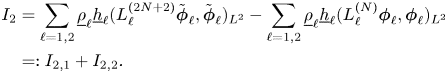
In view of (3.8), we see that

where we used $L_{\ell,ij}^*=L_{\ell,ji}$ . Similarly, we see also that

Here, it follows from (3.8) that $H_1^{2j}\mathcal {L}_{1,0}^{(N)}\boldsymbol {\phi }_1 = \sum _{i=0}^NL_{1,ji}\phi _{1,i}$ and $H_2^{p_j}\mathcal {L}_{2,0}^{(N)}\boldsymbol {\phi }_1 = \sum _{i=0}^{N^*}L_{2,ji}\phi _{2,i}$
 hold only for $j=0,1,\ldots,N$
 and for $j=0,1,\ldots,N^*$
 , respectively. Therefore, we have

so that
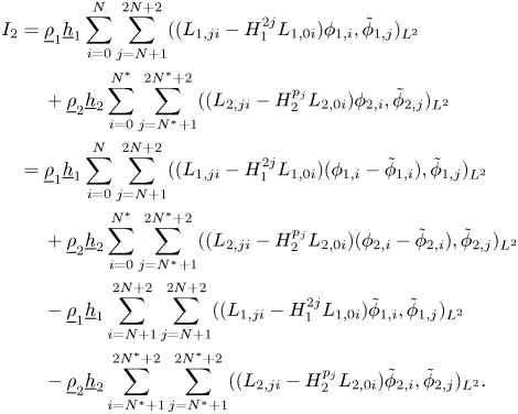
Hence, denoting by $\boldsymbol {\varphi }_1=(\varphi _{1,0},\varphi _{1,1},\ldots,\varphi _{1,N})^\mathrm {T}$ and $\boldsymbol {\varphi }_2=(\varphi _{2,0},\varphi _{2,1},\ldots,\varphi _{2,N^*})^\mathrm {T}$
 with $\varphi _{\ell,i}=\phi _{\ell,i}-\tilde {\phi }_{\ell,i}$
 we obtain

Here, we note that $(\boldsymbol {\varphi }_1,\boldsymbol {\varphi }_2)$ satisfy

where
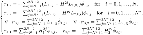
We put $\boldsymbol {r}_1'=(0,r_{1,1},\ldots,r_{1,N})^\mathrm {T}$ and $\boldsymbol {r}_2'=(0,r_{2,1},\ldots,r_{2,N})^\mathrm {T}$
 . Then, with a suitable decomposition $\boldsymbol {r}_\ell =\boldsymbol {r}_\ell ^\mathrm {high}+(\underline {h}_\ell \delta )^{-2}\boldsymbol {r}_\ell ^\mathrm {low}$
 for $\ell =1,2$
 , and using the linearity of (5.1), we see by lemma 5.1 that

Moreover, it follows from [Reference Iguchi19, lemmas 5.2 and 5.4] that

for $k=0,2$ , and hence also for $k=1$
 by interpolation, so that

where we used lemma 5.1 with (2.15), and interpolation. This completes the proof of theorem 3.10.
Acknowledgements
T. I. was partially supported by JSPS KAKENHI grant number JP17K18742 and JP22H01133. V. D. thanks the Centre Henri Lebesgue ANR-11-LABX-0020-01 for creating an attractive mathematical environment.


