


1. Introduction
Unsteady aerodynamics of airfoils has received substantial interest for its universality in nature and engineering fields, such as flapping wings, rotating and pitching blades on wind turbines and aircraft disturbed by turbulence or gusts. These flow phenomena, simplified as the unsteady flow problem around the airfoil (McCroskey Reference Mccroskey1982), can be generally divided into two categories. One is the stationary airfoil with unsteady incoming flow, and the other is the motion airfoil with a uniform free stream.
Due to the universality and importance of the unsteady flow problem, many scholars have devoted themselves to theoretical research on this problem since the last century (Leishman Reference Leishman2006). The early researchers include Wagner (Reference Wagner1925) and Küssner (Reference Küssner1936). The exact and complete analysis of a flat plate in harmonic oscillation was first given by Theodorsen (Reference Theodorsen1935). Later, Sears (Reference Sears1938, Reference Sears1941) derived the unsteady force formula for an airfoil passing through a sinusoidal vertical gust. The two theories are based on the thin-airfoil theory and the small perturbation assumption and are commonly used in the engineering community (Dowell Reference Dowell2014). As an extension of Theodorsen's theory, Greenberg (Reference Greenberg1947) developed a reduced model involving harmonic oscillation of an airfoil in sinusoidal streamwise gusts. Goldstein & Atassi (Reference Goldstein and Atassi1976) and Atassi (Reference Atassi1984) extended Sears’ theory to a second-order model considering the influence of airfoil camber and angle of attack. Lysak, Capone & Jonson (Reference Lysak, Capone and Jonson2013) corrected the Sears theory for predicting the unsteady lift forces considering the effect of airfoil thickness.
Although theoretical models have been developed for decades, these theories have not been widely validated experimentally until recent years, especially Theodorsen's and Sears’ theories. Ol et al. (Reference Ol, Bernal, Kang and Shyy2009) investigated the unsteady lift of an oscillating SD7003 airfoil using both experiments and numerical computation. The reduced frequency ( ${k_m={\rm \pi} f_mc/U}$) of airfoil oscillation was 0.25, where fm is the frequency of the airfoil motion, c is the chord length of the airfoil and U represents the free-stream velocity. They found that the lift coefficients obtained by experiment, computation and Theodorsen's theory were comparable. Even under deep stall conditions, theoretical predictions exhibited minimal deviation. Chiereghin, Cleaver & Gursul (Reference Chiereghin, Cleaver and Gursul2019) chose the NACA 0012 airfoil to study the unsteady response of the periodically plunging airfoil at a Reynolds number of Re = 20 000. The reduced frequency was km ≤ 1.1, and the mean angle of attack was 0–20°. They found that the theory can predict the amplitude and phase of the lift force well, regardless of whether the leading-edge vortex appears, although the increase in the time average of the lift caused by vortex lift cannot be captured. Considering the thin-airfoil theory assumptions, Cordes et al. (Reference Cordes, Kampers, Meiner, Tropea, Peinke and Hölling2017) studied a pitching Clark-Y airfoil with small oscillation amplitude at a reduced frequency of km = 0.025–3. The pitching amplitude αm varied from 2° to 6°, and the average angle of attack ranged from −4° to 8°. They found that the experimental and theoretical values agreed best when the average angle of attack was equal to the zero-lift angle of attack. The difference between the experimental and theoretical values increased as the average angle of attack increased. In contrast, the pitching amplitude had little effect on theoretical prediction accuracy.
Perhaps due to the difficulty in creating good sinusoidal vertical gust inflow conditions, a significant deviation has been observed in many early attempts to verify Sears’ theory (Hakkinen & Richardson Reference Hakkinen and Richardson1957; Commerford & Carta Reference Commerford and Carta1974). Jancauskas & Melbourne (Reference Jancauskas and Melbourne1986) used two airfoils with controllable circulation to generate sinusoidal vertical gusts and found that the experimental data exhibited good agreement with Sears’ prediction. Cordes et al. (Reference Cordes, Kampers, Meiner, Tropea, Peinke and Hölling2017) measured the Clark-Y airfoil's response to a sinusoidal vertical gust and found that the experimental measurements were generally opposite to Sears’ theory. However, it was later clarified by Wei et al. (Reference Wei, Kissing, Wester, Wegt, Schiffmann, Jakirlic, Hölling, Peinke and Tropea2019) that the gust in their facility did not meet Sears’ inflow conditions. Wei et al. (Reference Wei, Kissing, Wester, Wegt, Schiffmann, Jakirlic, Hölling, Peinke and Tropea2019) tested Sears’ theory in the range of reduced frequency ( $k_g={\rm \pi} f_gc/U$) from 0.09 to 0.42, where fg is the frequency of incoming flow oscillation. Their experimental results followed the general trend of Sears’ prediction within the reduced frequency of $k_g > 0.2$. However, a significant deviation was observed when the reduced frequency kg was less than 0.15.
Existing studies have confirmed the application of Theodorsen's and Sears’ theories. However, the problems involved in the two theories are relatively ideal. For more complex disturbance phenomena, such as the simultaneous existence of model motion and incoming flow disturbance (Liu et al. Reference Liu, He, He, Wang and Chen2021), a corresponding theoretical model is lacking. This problem is particularly relevant to micro air vehicles (MAVs) (Jones, Cetiner & Smith Reference Jones, Cetiner and Smith2022). The MAVs with flapping wings, designed in imitation of birds, have excellent aerodynamic performance and overcome the problem of insufficient lift occurring in traditional fixed-wing aircraft at low Reynolds numbers (Mueller Reference Mueller2001; Platzer et al. Reference Platzer, Jones, Young and Lai2008; Wang et al. Reference Wang, He, He, Wang, Chen and Liu2022). However, when faced with complex incoming disturbances, MAVs cannot cope well like a bird (Watkins et al. Reference Watkins, Milbank, Loxton and Melbourne2006; Quinn et al. Reference Quinn, Kress, Chang, Stein, Wegrzynski and Lentink2019). The coupling effect of the wing motion and the unsteady incoming flow could cause a large unsteady load, which greatly affects the safety and controllability of the aircraft. Therefore, predicting the aerodynamic force of the airfoil under the combined disturbances is of great significance for the design of aerodynamic components and flight control.
So far, Greenberg's theory may be the only aerodynamic model that simultaneously considers airfoil motion and unsteady incoming disturbance. Recently, Ma et al. (Reference Ma, Yang, Li and Li2021) experimentally studied an oscillating airfoil encountering sinusoidal streamwise gusts and compared the results with Greenberg's theory. They observed an overall trend of agreement between the experimental results and Greenberg's prediction, with only a minor deviation in the lift coefficient amplitude. Compared with the streamwise gust emphasized by Greenberg's theory, the vertical gust has a more significant impact on the aerodynamic force of the airfoil, so it deserves more attention. In the present study, a theoretical model is derived based on Theodorsen's and Sears’ theories involving a motion airfoil entering vertical gusts. The unsteady lift of a pitching airfoil encountering a sinusoidal vertical gust is experimentally studied to verify the applicability of the theoretical model. Moreover, the theoretical model is further modified through the steady experimental results, which provides actionable insights for engineering applications. The velocity fields are statistically analysed to unveil the underlying flow mechanisms to which the theoretical framework is applicable.
2. Theoretical description
In this section, a brief overview of the derivation process of Theodorsen's and Sears’ formulas is presented to illustrate the rationality of linear combination theory.
In the past century, researchers have made many efforts to predict the unsteady aerodynamic force of airfoils. At first, this kind of unsteady problem was solved based on the quasi-steady thin-airfoil theory. The quasi-steady thin-airfoil theory assumes that the flow is inviscid, incompressible and attached, with the thickness of the airfoil being negligible. The vortex sheet model for a symmetrical airfoil is shown in figure 1. The free-stream velocity is U, and the airfoil is simplified as a thin plate, which is replaced by a series of point vortices whose strength  $\gamma_{0}$ varies with position. When dealing with the boundary condition around the airfoil, not only instantaneous angle of attack, but also the relative motion of the fluid and the airfoil is considered. The strength of the vortex street is determined by the boundary condition and the Kutta condition. Furthermore, the quasi-steady lift of the airfoil can be obtained through the Kutta–Joukowski theory as
 \begin{equation}{L_0} = \rho U\!\varGamma_0 = \rho U\int_{ - c/2}^{c/2} {{\gamma _0}(x)\,\textrm{d}\kern0.7pt x} .\end{equation}
Here, ρ is the fluid density, and  $\varGamma\!$0 is the circulation around the airfoil.

Figure 1. Vortex sheet model based on thin-airfoil theory.
Under unsteady conditions, the circulation around the airfoil is constantly changing. According to Kelvin's circulation theorem, an attached vortex must detach from the trailing edge of the airfoil and be carried downstream at the local flow speed, forming the so-called ‘wake vortex’. Obviously, the quasi-steady thin-airfoil theory ignores the influence of the wake vortex at the trailing edge of the airfoil, which limits its accurate prediction of unsteady aerodynamic forces. Therefore, the unsteady thin-airfoil theory came into being.
A general method for determining unsteady lift based on unsteady thin-airfoil theory was presented by Sears (Reference Sears1938). This theoretical framework reproduces the results proposed by Wagner (Reference Wagner1925), Küssner (Reference Küssner1936) and Theodorsen (Reference Theodorsen1935).
In Sears’ theoretical framework, the influence of wake is considered, and the potential flow field around the airfoil is computed by continuously point vortices along the airfoil and its wake. The vortex sheet model is shown in figure 2. The vortex strength  $\gamma_{w}$ in the wake region induces velocities on the airfoil surface, resulting in a new wall boundary condition that must be satisfied. Therefore, the vortex strength on the airfoil consists of two parts, the quasi-steady component $\gamma_{0}$ and the component $\gamma_{1}$ induced by the wake vortex. Through a series of derivations, Sears obtained the general formula for calculating the unsteady aerodynamic force of the airfoil. For an airfoil with a chord length of c, when the coordinate origin is fixed at the middle chord point, the general formula for the unsteady lift of the airfoil can be expressed as follows:
 \begin{equation}L = {L_0} - \rho \frac{\textrm{d}}{{\textrm{d}t}}\int_{ - c/2}^{c/2} {{\gamma _0}(x)x\,\textrm{d}\kern0.7pt x} + \rho U\int_{c/2}^\infty {{\gamma _w}(x)} \frac{{c/2}}{{\sqrt {(x + c/2)(x - c/2)} }}\,\textrm{d}\kern0.7pt x.\end{equation}
As shown in (2.2), unsteady lift consists of three components. The first term is called the quasi-steady term, which is equal to the quasi-steady force obtained by (2.1); the second term is the added mass term, which is related to the unsteady change of the quasi-steady vortex intensity on the airfoil; the third term, related to the wake vortex, is called the wake effect term. It can be seen that the key to calculating the unsteady lift of the airfoil is to solve the quasi-steady vortex intensity  $\gamma_{0}$ and the wake vortex intensity $\gamma_{w}$.

Figure 2. Vortex sheet model considering the effect of wake.
Starting from (2.2), Sears (Reference Sears1941) analysed the sinusoidal oscillating airfoil and reproduced the lift expression derived by Theodorsen (Reference Theodorsen1935). For the pure sinusoidal pitching airfoil, with a change of the angle of attack according to  $\alpha=\alpha_m\sin(2{\rm \pi} f_mt)$, where αm is the pitching angle amplitude and fm is the pitching frequency, the unsteady lift of the airfoil can be written as
 \begin{equation}
{L_m} = \frac{{\rm \pi}
}{4}\rho {c^2}\Bigl[{U\dot{\alpha } + \Big( {\frac{1}{2}
- \frac{{{x_p}}}{c}} \Big)c\ddot{\alpha }} \Bigr] + {\rm \pi}
\rho c{U^2}\Bigl[ {\alpha + \Big( {\frac{3}{4} - \frac{{{x_p}}}{c}} \Big)\frac{c}{U}\dot{\alpha }}
\Bigr]C({k_m}).\end{equation}
\begin{equation}
{L_m} = \frac{{\rm \pi}
}{4}\rho {c^2}\Bigl[{U\dot{\alpha } + \Big( {\frac{1}{2}
- \frac{{{x_p}}}{c}} \Big)c\ddot{\alpha }} \Bigr] + {\rm \pi}
\rho c{U^2}\Bigl[ {\alpha + \Big( {\frac{3}{4} - \frac{{{x_p}}}{c}} \Big)\frac{c}{U}\dot{\alpha }}
\Bigr]C({k_m}).\end{equation}
Here,  $\dot{\alpha }$ and $\ddot{\alpha }$ are the first and second derivatives of the angle of attack with time, xp is the distance from the pitching axis to the leading edge of the airfoil, km is the reduced frequency of the pitching motion, as defined in the Introduction, and C(km) is the well-known Theodorsen function (Leishman Reference Leishman2006). Unlike Sears’ classification, Theodorsen divided unsteady lift into two parts, the non-circulatory force and circulatory force, corresponding to the first and second terms in (2.3), respectively. According to Sears’ solution process, the first term of (2.3) is derived from the added mass term in (2.2), and the second term is derived from the sum of the quasi-steady term and the wake effect term. This means that the non-circulatory force corresponds to the added mass term, while the circulatory force is equivalent to the addition of the quasi-steady term and the wake effect term.
In addition, Sears analysed the problem of airfoils subjected to sinusoidal vertical gust disturbances for the first time. The vertical component of the incoming flow velocity is expressed as  $v = \hat{v}\sin [2{\rm \pi} {f_g}(t - x/U + \phi )]$, where fg represents the gust frequency, $\hat{v}$ represents the gust amplitude and ϕ is the vertical gust phase at the position x = 0 at the initial moment. Referring to the work of Sears (Reference Sears1941) and considering the influence of the gust phase, the unsteady lift response of an airfoil can be calculated as
 \begin{equation}{L_g} = {\rm \pi}\rho cU\hat{v}\,{\textrm{e}^{\textrm{i}(2{\rm \pi} {f_g}t + \phi )}}S({k_g}) \approx {\rm \pi}\rho c{U^2}{\hat{\alpha }_g}\,{\textrm{e}^{\textrm{i}(2{\rm \pi} {f_g}t + \phi )}}S({k_g}).\end{equation}
Here, kg is the reduced frequency of gust defined in the Introduction, S(kg) is the famous Sears function (Leishman Reference Leishman2006) and  ${\hat{\alpha }_g} = \arctan (\hat{v}/U)$ is called the gust angle magnitude. When $\hat{v} \ll U$, ${\hat{\alpha }_g}$ is approximately proportional to $\hat{v}$.
As mentioned above, the issue solely pertaining to airfoil motion or gust disturbance can be described by the vortex sheet model shown in figure 2. Therefore, the two types of problems are inherently superimposed, that is, the linear addition of point vortices in two types of independent problems is a reasonable description of the combined problem. In the general formula of the unsteady lift given by (2.2), each term is linearly dependent on point vortex strength. Therefore, for the combined problem of airfoil motion and vertical gust disturbance, the theoretical unsteady lift of the airfoil can be obtained by linearly adding the theoretical lift of the two independent problems.
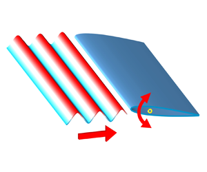
For a harmonic pitching airfoil encountering a sinusoidal vertical gust, as shown in figure 3, the theoretical formula of unsteady lift can be obtained by adding (2.3) and (2.4). The lift force is normalized by dynamic pressure to give the lift coefficient as
 \begin{align}{C_L} = \frac{{\rm \pi} }{2}c\left[ {\frac{{\dot{\alpha }}}{U} + \left( {\frac{1}{2} - \frac{{{x_p}}}{c}} \right)\frac{{\ddot{\alpha }}}{U}} \right] + 2{\rm \pi} \left[ {\alpha + \left( {\frac{3}{4} - \frac{{{x_p}}}{c}} \right)\frac{c}{U}\dot{\alpha }} \right]C({k_m}) + 2{\rm \pi} {\hat{\alpha }_g}\,{\textrm{e}^{\textrm{i}(2{\rm \pi} {f_g}t + \phi )}}S({k_g}).\end{align}
In the above formula, the first two terms are the lift caused by the airfoil motion, denoted as CL,M and the last term is the lift caused by the gust, denoted as CL,G.

Figure 3. Vertical gust flow over a pitching airfoil.
3. Experimental methods
3.1. Experimental device
The experiments were carried out in the low-speed water tunnel of Beijing University of Aeronautics and Astronautics. The test section had a cross-sectional profile of 1.0 m × 1.2 m. The maximum achievable free-stream velocity is 0.5 m s−1. A gust device was installed 0.78 m upstream of the test model and composed of two pitching blades with adjustable motion modes, as shown in figure 4. The spacing between the two blades is 0.38 m. Each blade has a NACA 0015 cross-sectional profile with a chord length of 0.24 m and a spanwise length of 0.6 m. Driven by two servo motors, the two blades can pitch simultaneously about their central chord points in sinusoidal profile. Compared with the downstream test airfoil, the gust blade exhibits a greater chord length and a thicker profile. These chosen blade parameters are intended to induce a more pronounced gust effect. Despite the larger chord length of the gust blade, implying an extended range of wake disturbance, the augmented blade spacing has been meticulously determined to ensure a constrained influence of the blade wake on the downstream measurement area (Wang & Feng Reference Wang and Feng2022).

Figure 4. (a) Three-dimensional diagram of the experimental device; (b) top view of the experimental device.
A NACA 0012 wing with a chord length c = 0.12 m and a span of 0.6 m was installed downstream as a test model. At zero angle of attack, the chord of the airfoil is aligned with the symmetry line of the two blades. The airfoil was made of solid aluminium to ensure sufficient stiffness under the unsteady load. The upper end of the model was connected to the force sensor. An endplate was fixed to the lower end to restrain the flow around the wing tip, and the interval between the endplate and the model was approximately 3 mm. Driven by a servo motor, the airfoil can perform sinusoidal pitching motion around its quarter chord line point in terms of specified oscillation frequencies fm and amplitudes αm. It is worth noting that the motors driving the gust device and the downstream airfoil were controlled by the same controller, so precise synchronous motion or specified phase difference motion can be achieved.
3.2. Force and flow field measurements
The aerodynamic force was measured by a six-component force/torque transducer with a data acquisition card at a frequency of 2000 Hz. The resolution of the force sensor was 5 × 10⁻³ N. Under the control of a synchronizer, the force signal was recorded at the moment that the airfoil starts to move. For each parameter combination, 100 continuous gust periods were measured. To obtain the unsteady lift, the force data were shifted from the airfoil frame of reference to that of the water tunnel. The first two periods of every set were removed to avoid any start-up effects. A Fourier transform of the signal yielded the magnitude of the lift-force fluctuations. In order to clearly show the time history of the lift, the instantaneous lift coefficient was processed by a finite impulse response (FIR) low-pass filter with a cutoff frequency of 15fg. Nevertheless, the frequency spectrum analysis of the lift was based on the original force data. The reliability of the force sensor in measuring the unsteady force has been verified in previous research (Wang, Feng & Li Reference Wang, Feng and Li2021; He et al. Reference He, Guo, Xu, Feng and Wang2023).
A two-dimensional particle image velocimetry (PIV) system was employed to record the vertical gust velocity in the absence of the downstream airfoil and to capture flow field information during the airfoil pitching motion. A continuous-wave Nd:YAG laser with a power of 8 W was used to light from one side of the wing, which caused the light on the other side of the wing to be blocked, so that flow field under the airfoil was not visible in the image, as shown in figure 4. Hollow glass beads with a diameter of 20 μm and a density of 1.05 g cm−3 were seeded in the water to accurately follow the flow. The measured section, situated at the mid-span of the airfoil, was captured by a high-speed camera (Photron Fastcam SA2 86K-M3) boasting a resolution of 2048 × 2048 pixels. For each case, a total of 54 cycles with 200 pairs of phase-locked images per cycle were recorded. Velocity fields were computed from the original images using the multi-pass iterative Lucas–Kanade algorithm (Champagnat et al. Reference Champagnat, Plyer, Le Besnerais, Leclaire, Davoust and Le Sant2011; Pan et al. Reference Pan, Xue, Xu, Wang and Wei2015). The interrogation window size was set to 32 × 32 pixels, with a 75 % overlap rate, ensuring a minimum of four particles per window. With a sampling rate of 200 Hz and an image magnification of 0.082 mm pixel−1, the computed velocity uncertainty was approximately 1.6 mm s−1.
3.3. Experimental parameters
In the experiment, the free-stream velocity was held at U = 0.2 m s−1, corresponding to a chord-based Reynolds number Re = 24 000. The turbulence intensity of the free stream was less than 1 %. Figure 5 shows the vertical velocity measured at the leading edge of the test airfoil with the airfoil absent. The gust frequency is fg = 0.11 Hz, and the corresponding period is recorded as Tg. Throughout this paper, these two quantities will be used to normalize frequency and time, respectively. It is clear from figure 5(a) that the vertical velocity profile matches well with a sine curve. The curve expression is  $v/U = 0.054\sin (2{\rm \pi} t/{T_g} - 0.13{\rm \pi} )$. The dimensionless vertical gust amplitude is 0.054, corresponding to a gust angle amplitude of ${\hat{\alpha }_g} = 3.14\mathrm{^\circ }$. Considering that the gust convects downstream at the free-stream velocity U, the phase of the gust at the midpoint of the airfoil at the initial moment is $\phi=-0.19{\rm \pi}$, which is an important parameter in (2.5). As the downstream airfoil consistently undergoes sinusoidal motion with a zero initial phase, ϕ can also serve as a representation of the phase difference between the gust and the airfoil motion. This value can be altered by delaying the movement of the gust blades relative to the downstream airfoil. Figure 5(b) shows the spectral analysis of the time history of the velocity. It can be seen that there is only one marked peak in the spectra. Therefore, the sinusoidal vertical gust produced by the gust generator has high signal-to-noise ratio. The gust uniformity in the transverse plane and spanwise direction has been evaluated in previous studies. The results distinctly indicated that the gust profiles had good consistency in all directions.

Figure 5. (a) Time history of the sinusoidal vertical gust and (b) the corresponding Fourier amplitude spectrum.
Under the above gust conditions, the aerodynamic response of the pitching airfoil was studied to examine the applicability of the theoretical model. When the pitching frequency differs from the gust frequency, a nonlinear effect may occur and lead to a more complex flow situation. Therefore, we considered two cases when selecting the experimental parameters: a particular case and a general case. In the particular case, the pitching frequency is the same as the gust ( fm = fg), while the pitching amplitude varies from 0° to 24°. In the general case, the pitching frequency differs from the gust frequency and is selected as fm = 0.5fg~2fg with the pitching amplitude held constant at αm = 4°.
4. Lift response prediction
4.1. Unsteady lift
The lift coefficients of the airfoils under two different cases are presented in figures 6 and 7. When the pitching frequency of the airfoil is equal to the gust frequency, the two disturbances are completely coupled. The lift coefficient changes periodically, and there is a unique primary frequency fg, as shown in figure 6. When the pitching frequency differs from the gust frequency, the lift coefficient still presents regular changes under multiple disturbances. In figure 7(a), the lift coefficient changes approximately with a period of  $2T_g$, which is precisely the common multiple of the gust and airfoil motion periods. In figure 7(b), in addition to the gust frequency and the airfoil motion frequency, a beat frequency equal to the difference between the two disturbance frequencies appears in the lift frequency spectrum, indicating a nonlinear effect between the disturbances caused by the gust and the pitching motion. Ma et al. (Reference Ma, Yang, Li and Li2021) also observed a similar frequency distribution law when studying the unsteady lift of an oscillating airfoil encountering a sinusoidal streamwise gust.

Figure 6. (a) Time history of the lift coefficient and (b) the corresponding Fourier amplitude spectrum for fm = fg and αm = 4°.

Figure 7. (a) Time history of the lift coefficient and (b) the corresponding Fourier amplitude spectrum for fm = 1.5fg and αm = 4°.
4.2. Comparison between theory and experiments
When the pitching frequency equals the gust frequency, the unsteady lift coefficient has only a single primary frequency, and the theoretical lift coefficient can be calculated according to (2.5). Figure 8 shows the measured lift coefficient amplitude and phase under different pitching amplitude conditions. It can be seen that the amplitude of the lift coefficient has the same variation trend as the theoretical value. Even in the range where the pitching amplitude exceeds the stall angle of attack, the theoretical value can still follow the experimental value very well. In the phase plot, the theoretical and experimental results are also in good agreement. It should be mentioned that figure 8 presents the results only for a gust phase of  $\phi=-0.19{\rm \pi}$.

Figure 8. (a) Amplitude and (b) phase of the unsteady lift coefficient for fm = fg. Experimental results for different αm are compared with theoretical prediction.
Considering that the phase difference between gust and airfoil motion is also an important parameter affecting the unsteady lift at fm = fg, we measured the unsteady force of the airfoil under different gust phases. Figure 9(a) displays the variation of gust velocity and airfoil angle of attack within one cycle. Altering the timing of gust generation allows for the manipulation of the phase difference between the two disturbance signals. For the case of  $\phi=-0.19{\rm \pi}$, the peak positions of the two signals are in close proximity, resulting in a larger lift amplitude under the coupling disturbance. When the phase difference reaches $-1.19{\rm \pi}$, the two signals exhibit near reversal, leading to a decrease in the lift amplitude. The theoretical prediction depicted in figure 9(b) effectively captures the trend in the lift amplitude measured in the experiment. The accuracy of the theoretical prediction remains relatively consistent across various phase difference conditions, with a slight overestimation in the amplitude. This demonstrates the theoretical model's capability to predict lift when the airfoil motion frequency aligns with the gust frequency.

Figure 9. Effect of the phase difference between gust and pitching on lift coefficient amplitude for fm = fg: (a) phase relationship between gust and airfoil motion; (b) amplitude of the unsteady lift coefficient for different ϕ at αm = 4°, 12°, and 24°.
When the pitching frequency deviates from the gust frequency, the lift coefficient is influenced by multiple frequencies, rendering a single amplitude and phase inadequate to capture the characteristics of unsteady lift. Figure 10 illustrates the comparison between the measured unsteady lift coefficient and the theoretical prediction for fm ≠ fg, and figures 10(a)–10(c) present the results for the pitching frequencies of fm = 0.75fg, 1.5fg and 2fg, respectively. For the sake of clarity, only several periods are displayed for each case. In general, despite the lift coefficient not exhibiting a simple harmonic pattern, the theory still accurately captures the trend of the lift. However, the disparity between the experimental results and theoretical predictions becomes significant, particularly at the instances of maximum and minimum lift coefficients.

Figure 10. Time history of the unsteady lift coefficient for fm ≠ fg and αm = 4°. Experimental results for (a) fm = 0.75fg, (b) fm = 1.5fg and (c) fm = 2fg are compared with theoretical predictions.
Figure 11 shows the frequency spectrum of the unsteady lift coefficient for fm ≠ fg. The dominant frequencies and the corresponding magnitudes are comparable between experiment and theory. According to the experimental results, the lift coefficient is dominated by the three frequencies: the gust frequency, airfoil motion frequency and beat frequency. The theory accurately predicts the first two frequencies, but it fails to predict the third one. This is because that theory is based on a linear superposition, which prevents it from capturing nonlinear products. The experimental results show three primary frequencies for the cases of fm = 0.75fg and fm = 1.5fg, whereas there are only two frequencies for the case of fm = 2fg. This does not imply that the nonlinear phenomenon exists solely for fm = 0.75fg and fm = 1.5fg; rather, in the latter case, the beat frequency coincides with the gust frequency and becomes indistinguishable.

Figure 11. The Fourier amplitude spectrum of the unsteady lift coefficient for fm ≠ fg and αm = 4°. Experimental results for (a) fm = 0.75fg, (b) fm = 1.5fg and (c) fm = 2fg are compared with theoretical predictions. The frequency bands marked by black dashed lines are utilized for reconstructing the lift coefficient, as depicted in figure 12.

Figure 12. Comparison of the lift coefficient between experimental results and reconstructed results from the gust frequency and pitching frequency for (a) fm = 0.75fg, (b) fm = 1.5fg and (c) fm = 2fg.
An interesting question pertains to the extent to which the beat frequency influences the lift coefficient. Undoubtedly, clarifying this matter holds substantial importance in delineating the appropriate application scenarios of the linear theory. In pursuit of addressing this inquiry, we conduct a further analysis focusing on the frequency-dependent lift coefficient. Starting from the frequency spectrum of the lift coefficient, a frequency band encompassing the two primary frequencies, namely the pitching frequency ( fm) and gust frequency ( fg), is selected for reconstructing the lift coefficient. Taking the case of fm = 0.75fg, 1.5fg and 2fg as examples, the frequency range delineated by the black dashed line in the figure 11 encloses the two primary perturbation frequencies and is utilized for the reconstruction of force signals. In order to minimize interference from extraneous frequencies, we chose a minimal frequency band that exclusively encompasses the two frequencies. For other cases, the selection of frequency bands follows the same principle.
Figure 12 provides a comparison between the reconstructed force signal based on the two primary frequencies and the original signal. Despite slight discrepancies, the reconstructed signal closely aligns with the experimental signal on the whole. For the cases of fm = 0.75fg and 1.5fg, the beat frequency emerges in the corresponding frequency spectrum of lift coefficient as presented in figures 11(a) and 11(b). The reconstructed lift exhibits a comparable trend to the original signal, suggesting that the beat frequency exerts a minor effect on the lift coefficient. For the case of fm = 2fg, only two distinct main frequencies are evident in the frequency spectrum. Consequently, the reconstructed signal closely mirrors the original signal. A comparative analysis of the initial two cases with the latter case reveals that the beat frequency does influence the overall lift coefficient, but this impact is minor.
To quantify the disparity between the reconstructed signal and the original signal, we calculated the root-mean-square (r.m.s.) of the lift coefficient fluctuations. Figure 13 presents a comparison between the original and reconstructed lift coefficients. It is discernible that, in all instances, the r.m.s. of the lift coefficient fluctuation falls within the range of 0.2 to 0.3. The reconstructed signal closely aligns with the original signal, with the maximum discrepancy not exceeding 1.5 %, as observed in the case of km = 0.3. These quantitative findings affirm that frequencies beyond the two primary perturbation frequencies have a weak influence on the lift coefficient. This underscores the crucial role of linear theory in predicting airfoil lift under multi-disturbance conditions. Given the minimal effect of the beat frequency on overall lift, it will be disregarded in subsequent quantitative comparison between theory and experiment.

Figure 13. Comparison of the r.m.s. lift coefficient fluctuations between experimental results and reconstructed results for fm ≠ fg and αm = 4°.
To quantify the difference of each part between the experimental results and theoretical values, we calculate the amplitudes and phases of the lift coefficient corresponding to the gust frequency and pitching frequency as given in figure 14. Each plot represents the amplitude and phase of every ‘dominant’ harmonic in the unsteady lift. The amplitude of the lift coefficient of each frequency has the same variation trend as the theory, while the lift amplitude is overestimated. The theoretical phase angles are generally consistent with the experimental results, with only minor deviations. Since the gust inflow condition was not changed in the experiment, the gust-induced lift amplitude and phase obtained theoretically remain constant. However, in the experimental results, the phase angle of the gust-induced lift tends to decrease as the pitching frequency increases, which is similar to the phase angle trend of motion-induced lift. This indicates that the airfoil motion may have a stronger disturbance to the incoming flow at a higher pitching frequency. However, due to the relatively few experimental conditions at present, more precise conclusions still need more substantial parametric studies.

Figure 14. Amplitudes and phases of the lift coefficient corresponding to (a,c) gust component and (b,d) pitching component for fm ≠ fg and αm = 4°. Experimental results for different km are compared with theoretical predictions.
4.3. Theoretical correction
From the above results, it can be seen that, although the theoretical model can predict the trend of the unsteady lift force, there are still apparent deviations in the lift coefficient amplitude. Therefore, some modifications to the theoretical model are necessary. By introducing the pivot position parameter xp = 0.25c and the pitching angle function  $\alpha=\alpha_m\sin(2{\rm \pi} f_mt)$ and combining the first two items, (2.5) can be rewritten as
 \begin{equation}{C_L} = 2{\rm \pi} {\alpha _m}\,{\textrm{e}^{\textrm{i}2{\rm \pi} {f_m}t}}\left[ {(1 + i{k_m})C({k_m}) + \frac{{i{k_m}}}{2} - \frac{1}{4}k_m^2} \right] + 2{\rm \pi} {\hat{\alpha }_g}\,{\textrm{e}^{\textrm{i}(2{\rm \pi} {f_g}t + \phi )}}S({k_g}).\end{equation}
Both terms of the above formula can be regarded as the product of the steady lift and transfer function. For the first term, the steady lift part is  $2{\rm \pi} {\alpha _m}\,{\textrm{e}^{\textrm{i}2{\rm \pi} {f_m}t}}$. For the second term, the steady lift part is $2{\rm \pi} {\hat{\alpha }_g}\,{\textrm{e}^{\textrm{i(}2{\rm \pi} {f_g}t + \phi )}}$. In the present experiment, it is evident from figure 15 that the steady lift coefficient of the airfoil deviates from the anticipated lift coefficient $2{\rm \pi}\alpha$. This discrepancy underscores an overestimation of the experimental quasi-steady lift by theoretical predictions. This divergence can be attributed to the theoretical model's foundational assumptions, premised on an inviscid flow and thin airfoil, which are not fully met under actual flow conditions. In particular, the significant viscosity at low Reynolds number will lead to a smaller steady lift coefficient. Similar phenomena have been observed in previous studies (Lee & Su Reference Lee and Su2012; Wang et al. Reference Wang, Zhou, Alam and Yang2014). Therefore, the theory formula is modified by substituting the steady term in (4.1) with the experimentally measured steady lift coefficient, which is obtained by interpolation of the lift coefficient in figure 15. The modification can be understood as a compensation for the deviation between the real flow and the ideal flow.

Figure 15. Variation of the lift coefficient with angle of attack for stationary airfoil.
Figure 16 compares the experimental and theoretical lift coefficient amplitudes for the same pitching and gust frequencies. It can be seen that the lift amplitude predicted by the modified model agrees very well with the experimental results, with only a tiny difference. Note that this theoretical correction works until the steady stall angle of attack. Above the stall angle of attack, significant flow separation occurs on the upper surface of the steady airfoil. In contrast, the unsteady airfoil can maintain attached flow due to the phenomenon of dynamic stall (Mulleners & Raffel Reference Mulleners and Raffel2013). This marked disparity in flow characteristics between steady and unsteady airfoils results in the modified theoretical model producing impractical predictions at larger angles of attack. When the pitching frequency is different from the gust frequency, both frequencies dominate the change of the lift coefficient. Therefore, the lift coefficient amplitudes corresponding to the gust frequency and pitching frequency are compared separately. In figure 17, each plot represents the amplitude of each ‘dominant’ harmonic in unsteady lift. For the gust-induced lift coefficient, the experimental results exhibit good agreement with the modified result. For the motion-induced lift coefficient, compared with the unmodified theory, the lift coefficient amplitudes predicted by the modified model are significantly closer to the experimental results, although differences still exist at a higher pitching frequency.

Figure 16. Amplitude of the unsteady lift coefficient for fm = fg. Experimental results for different αm are compared with modified theoretical prediction.

Figure 17. Amplitude of the unsteady lift coefficient corresponding to gust component and pitching component for fm ≠ fg and αm = 4°. Experimental results for different km are compared with modified theoretical predictions.
4.4. Lift coefficient normalization
When subjected to coupled gust and pitching disturbances, the lift coefficient of an airfoil is influenced by both the gust and the airfoil motion. The essence effect of the two disturbances on the airfoil is to change the effective angle of attack of the airfoil relative to the incoming flow. Previous studies (Biler, Badrya & Jones Reference Biler, Badrya and Jones2019; Li et al. Reference Li, Feng, Kissing, Tropea and Wang2020) have typically defined the effective angle of attack as the geometric attack angle of the airfoil for pitching disturbances and as the gust angle for vertical gust disturbances. However, these definitions overlook the unsteady effects caused by the wake vortex street. Therefore, we propose a new definition of the effective angle of attack based on the theoretical formula presented herein, aiming to elucidate the influence of coupled disturbances on the lift coefficient.
Starting with the theoretical equation (4.1), the effective angle of attack resulting from pitching motion is defined as
 \begin{equation}{\alpha _{m,eff}} = {\alpha _m}\,{\textrm{e}^{\textrm{i}2{\rm \pi} {f_m}t}}\left[ {(1 + i{k_m})C({k_m}) + \frac{{i{k_m}}}{2} - \frac{1}{4}k_m^2} \right].\end{equation}
The effective angle of attack caused by vertical gust is defined as
 \begin{equation}{\alpha _{g,eff}} = {\hat{\alpha }_g}\,{\textrm{e}^{\textrm{i}(2{\rm \pi} {f_g}t + \phi )}}S({k_g}).\end{equation}
Under the simultaneous influence of gust and pitching disturbances, the effective angle of attack of the airfoil is expressed as the sum of the two components above
 \begin{equation}{\alpha _{eff}} = {\alpha _{m,eff}} + {\alpha _{g,eff}}.\end{equation}
Combining this with (4.1), the total lift coefficient can be expressed as
 \begin{equation}{C_L} = 2{\rm \pi} {\alpha _{eff}}.\end{equation}
 This equation highlights that the lift coefficient is determined by the effective angle of attack αm,eff and αg,eff induced by airfoil motion and vertical gusts. When the gust and pitching frequencies are the same, the lift coefficient is dominated by a single frequency, and its amplitude is linearly related to the maximum effective angle of attack, max{αeff}. When the frequencies differ, the lift coefficient includes components corresponding to the gust and pitching frequencies. Specifically, the lift coefficient amplitude associated with the gust frequency,  ${\hat{C}_{L,G}}$, is related to the maximum effective angle of attack, max{αg,eff}, induced by vertical gusts, while the lift coefficient amplitude associated with the pitching frequency, ${\hat{C}_{L,M}}$, is related to the maximum effective angle of attack, max{αm,eff}, induced by pitching motion.
Figure 18 illustrates the relationship between the maximum effective angle of attack and measured lift amplitude under all various conditions. The effective angle of attack is determined through (4.2)–(4.4). For single-frequency disturbance cases, such as pitching disturbance alone or coupled pitching and gust disturbances with the same frequency, the abscissa is obtained by taking the maximum value of the effective angle of attack derived from (4.4). Under dual-frequency disturbance conditions involving coupled gust and pitching disturbances with different frequencies, the abscissae signify the maxima of the effective angle of attack induced by pitching and gusts. These maxima are ascertained by (4.2) and (4.3), respectively. Correspondingly, the ordinate represents the measured lift amplitudes of pitching and gust components. Notably, irrespective of variations in gust and pitching conditions, a linear relationship between the maximum effective angle of attack and the lift coefficient amplitude is observed.

Figure 18. Lift coefficient amplitude as a function of maximum effective angle of attack.
For coupled gust and pitching disturbance problem, a series of parameters affect the airfoil's lift response. These parameters encompass pitching frequency and amplitude, gust frequency and amplitude, as well as the phase difference between gust and pitching signals. Present theoretical and experimental findings demonstrate that the fundamental influence of these parameters on the lift coefficient lies in their alteration to the proposed effective angle of attack.
5. Flow field characteristics
The analysis in the previous section shows that the theory correction agrees very well with experimental values when the pitching frequency is low. As the pitching frequency increases, the lift amplitude associated with the pitching component progressively diverges from the theoretical prediction and tends to be overestimated. The applicability of the theory hinges fundamentally on the extent to which the two perturbations can be linearly superimposed. Therefore, this section delves deeper into elucidating the underlying flow mechanism that governs the applicability of the theory.
Figure 19 depicts the velocity field surrounding a pitching airfoil under different incoming flow conditions. In the absence of gusts (figures 19a–19c), the flow on the upper airfoil is dominated by attached flow throughout the entire pitching cycle. When subjected to vertical gusts (figures 19d–19f), the primary flow characteristics of the upper airfoil remain relatively consistent compared with the no-gust scenario. The discernible alterations induced by the gusts occur primarily in flow velocity above the airfoil. Figure 19(d) corresponds to the moment when the vertical gust attains its maximum positive value at the airfoil's leading edge. At this time, a notable increase in flow velocity above the airfoil occurs, accompanied by an expansion of the high-speed region. In figure 19(e), the vertical gust at the airfoil's leading edge diminishes to zero. Nevertheless, as the positive vertical gust has not yet convected away from the airfoil, the velocity amplitude above the upper airfoil remains considerably higher than in the no-gust condition of figure 19(b). In figure 19( f), when the vertical gust reaches its maximum negative value, the flow velocity over the upper airfoil surface diminishes in response to the vertical gust. This alteration in flow velocity results from the change of the effective angle of attack of the airfoil, which is closely related to vertical gusts. A reduction in the effective angle of attack results in the deceleration of the flow above the airfoil, while an increase accelerates the flow above the airfoil. However, the effective angle of attack can only offer qualitative insights into the changes in the flow over airfoil surface, lacking the quantitative predictive capability necessary to describe the flow field around the airfoil.

Figure 19. Velocity field around pitching airfoil with fm = fg and αm = 4° under (a–c) no gust and (d–f) vertical gust. The instantaneous gust signal encountered by the airfoil in (d–f) is marked on the upper right diagram. The white, green and blue dashed lines are isolines with velocity amplitudes of 1.15U, 1.1U and 1.05U, respectively.
According to the analysis in § 2, it can be seen that, under the combined pitching and gust disturbances, the lift coefficient of the airfoil is related to the scenarios where a single disturbance acts on the airfoil alone. Therefore, it is reasonable to speculate that a connection also exists between flow fields around the airfoil under combined disturbances and individual disturbances. For an airfoil that is only subject to a single vertical gust disturbance, namely the airfoil is stationary, the vortex sheet model considering the influence of the wake is shown in figure 20(a).

Figure 20. Schematic diagram of the vortex sheet model under different disturbance scenarios: (a) gust disturbance; (b) pitching disturbance.
According to the potential flow theory, the flow velocity in space is equal to the superposition of the velocities induced by different potential flow fields. Therefore, the velocity field around the airfoil under gust disturbance, noted as ug, can be determined by the following formula:
 \begin{equation}{\boldsymbol{u}_g} = \boldsymbol{U} + {\boldsymbol{v}_g} + \boldsymbol{u}({\gamma _{a,g}}) + \boldsymbol{u}({\gamma _{w,g}}),\end{equation}
where U represents the free-stream velocity, vg is the gust velocity and u( $\gamma_{a,g}$) and u( $\gamma_{w,g}$) stand for the velocities induced by the bound vortex $\gamma_{a,g}$ and wake vortex $\gamma_{w,g}$, respectively; $\gamma_{a,g}$ and $\gamma_{w,g}$ are linked to the gust disturbance.
For an airfoil undergoing only pitching disturbance, its angle of attack continually changes relative to the free stream. The vortex sheet model, accounting for the wake's influence, is depicted in figure 20(b). The velocity field around the airfoil under pitching disturbance, designated as um, can be expressed as
 \begin{equation}{\boldsymbol{u}_m} = \boldsymbol{U} + \boldsymbol{u}({\gamma _{a,m}}) + \boldsymbol{u}({\gamma _{w,m}}).\end{equation}
Here, u( $\gamma_{a,m}$) and u( $\gamma_{w,m}$) represent the velocities induced by the bound vortex $\gamma_{a,m}$ and wake vortex $\gamma_{w,m}$. Both $\gamma_{w,m}$ and $\gamma_{a,m}$ are associated with pitching disturbances.
For an airfoil encountering both gusts and pitching disturbances simultaneously, the velocity field around the airfoil ugm can be written as
 \begin{equation}{\boldsymbol{u}_{gm}} = \boldsymbol{U} + {\boldsymbol{v}_g}\boldsymbol{+ u}({\gamma _{a,g}}) + \boldsymbol{u}({\gamma _{a,m}})\boldsymbol{+ u}({\gamma _{w,g}}) + \boldsymbol{u}({\gamma _{w,m}}).\end{equation}
Based on (5.1)–(5.3), it is apparent that there exists a quantitative relationship among the flow fields around the airfoil in these three scenarios:
 \begin{equation}{\boldsymbol{u}_{gm}} = {\boldsymbol{u}_g}\boldsymbol{+ }{\boldsymbol{u}_m} - \boldsymbol{U}.\end{equation}
Equation (5.4) can be interpreted as follows: the velocity field under the combined gust and pitching disturbances is equivalent to the linear addition of the flow fields when the two disturbances act alone on the airfoil with the free-stream velocity subtracted. However, it should be noted that the vortex sheet model is based on the traditional thin-airfoil theory. Consequently, the derivation of (5.4) inherently assumes the presence of small pitching and gust perturbations. Furthermore, the theory posits that the airfoil is a thin, flat plate. In practice, however, even a zero-angle-of-attack airfoil, owing to its finite thickness, can influence the free-stream velocity field to some extent. To address this discrepancy, an empirical correction is introduced here. This correction substitutes the velocity field U in (5.1)–(5.4) with the experimentally measured flow field around a zero-angle-of-attack airfoil under a steady free stream. As a result, in scenarios devoid of both gust and pitching disturbances, (5.1)–(5.4) yield realistic results. To facilitate testing the aforementioned (5.4), the velocity fields were rotated into the airfoil reference system in the pitching disturbance scenario, with the origin of the coordinate axis always at the leading edge of the airfoil, and the x axis along the chord direction. This transformation, however, is predicated on small pitching amplitude, as it ignores the impact of pitching angle variations on the interaction between gust and the airfoil.
Figure 21 illustrates the velocity fluctuation surrounding the airfoil under three distinct disturbance conditions. Figures 21(a) and 21(d) depict the impact of gust disturbance alone, revealing that vertical velocity disturbances are predominantly concentrated in the upstream region near the airfoil. As the flow passes over the airfoil's leading edge, the velocity fluctuations shift from the vertical direction to the streamwise direction and decrease downstream rapidly. A gradual increase in velocity fluctuations is observed in the second half of the airfoil, which correlates with period changes in the shear thickness within this zone. A similar velocity fluctuation distribution emerges in the case of the pitching disturbance acting independently, as demonstrated in figures 21(b) and 21(e). Notably, velocity fluctuations are more pronounced in the vicinity of the airfoil under a pitching disturbance compared with a gust disturbance. When both pitching and gust disturbances emerge simultaneously, the velocity disturbances near the airfoil are markedly intensified, as depicted in figures 21(c) and 21( f).

Figure 21. Velocity fluctuation intensity around the airfoil under different disturbances in the airfoil coordinate system: (a,d) gust disturbance; (b,e) pitching disturbance; (c, f) combined gust and pitching disturbances (fm = fg and αm = 4°). The left column is the r.m.s. streamwise velocity fluctuation, and the right is the r.m.s. vertical velocity fluctuation.
To examine the linear relationship of velocity disturbances across different scenarios, we present velocity signals from six representative points in figure 22. Among these, three points – namely P1, P2 and P3 – are designated for streamwise velocity measurements. The streamwise velocity fluctuations at these points are markedly more pronounced in the case of double disturbances compared with single disturbances. Simultaneously, three additional points – P4, P5 and P6 – are chosen for vertical velocity measurements, following a similar selection rationale.

Figure 22. Time history of flow velocity at typical points around the airfoil in a single gust period under different disturbances: (a–c) the streamwise velocities of points P1–P3; (d–f) the vertical velocities of points P4–P6 (fm = fg and αm = 4°). These points are marked with black boxes in figure 21. The measured results of the combined disturbances are compared with the predicted results.
Figure 22(a) portrays the variations in streamwise velocity at point P1, where the streamwise velocity fluctuation is most pronounced near the leading edge under the double disturbance scenario. At all three different disturbance conditions, the streamwise velocity at point P1 exhibits an approximately sinusoidal profile. Notably, the streamwise velocity displays distinct phases and amplitudes for the two single disturbance scenarios. Nevertheless, the streamwise velocity changes predicted by the linear combination strategy closely align with the experimental results in the presence of double disturbances. Point P2 also experiences a significant increase in streamwise velocity fluctuation under double disturbances in figure 22(b), and a favourable agreement is observed between the measured and predicted results. At point P3, situated in the middle chord of the airfoil, the streamwise velocity deviates from its sinusoidal trend, as illustrated in figure 22(c). When the streamwise velocity is higher, the predicted and measured results exhibit a similar trend; however, differences emerge as the flow velocity decreases. This discrepancy arises because point P3 occasionally resides within the airfoil's boundary layer, such as the instant corresponding to figure 19(d). The presence of wall viscosity reduces the actual measured velocity at this point, accounting for the observed differences. Different from the distribution of streamwise velocity, the vertical velocity fluctuations are most prominent just upstream of the airfoil's leading edge and rapidly diminish after reaching the upper surface of the airfoil. It can be seen from figures 22(d)–22( f) that the predicted velocity signal accurately follows the experiment results. These findings affirm the applicability of linear superposition in the flow field. Leveraging this approach, it becomes feasible to predict the principal characteristics of the flow field under coupled disturbances through the linear superposition of individual perturbation flow fields.
To assess the generality of disturbance superposition, we further investigate scenarios where gust and pitching disturbances have different frequencies. Figures 23(a) and 23(b) provide a comparative analysis of the streamwise velocity at the leading-edge point under distinct disturbances when fm = 0.75fg and fm = 2fg, respectively. Notably, although the streamwise velocity exhibits a complex pattern under individual disturbances, the alterations in flow velocity under combined disturbances remain consistent with the prediction results of the linear combination. This strong consistency serves as a robust validation of the practicality of the combined vortex sheet model and offers further insights into why the combined Theodorsen and Sears theory remains applicable. An intriguing revelation emerges when comparing the streamwise velocity curve at the leading-edge point under coupled disturbances with the lift variation curve in figure 10. Specifically, the comparison between figures 23(a) and 10(a), as well as figures 23(b) and 10(c), reveals highly similar trends in both datasets. This observation implies that alterations in flow velocity near the airfoil's leading edge may serve as an indicator for predicting variations in the lift coefficient under small disturbances.

Figure 23. Time history of streamwise velocity above the airfoil's leading edge under different disturbance conditions for (a) fm = 0.75fg and (b) fm = 2fg. The velocity measurement point is located at the local maximum streamwise velocity fluctuation under combined disturbances.
In the preceding section, we observed that, as pitching frequency increases, the lift amplitude associated with the pitching component diminishes compared with the theoretical values. In order to explore the underlying flow mechanism, the flow field information corresponding to the pitching component is extracted. Figure 24 compares the velocity fluctuation amplitude corresponding to the pitching frequency component under different perturbations. The reduced frequency of the pitching perturbation is km = 0.15, which is 0.75 times the gust reduced frequency. The velocity fluctuation amplitude is determined by extracting the amplitude of the local flow velocity corresponding to the pitching frequency component. It should be noted that two airfoils are drawn in each cloud diagram, corresponding to the maximum and minimum pitching angle instants. Only outside the boundaries of these two airfoil profiles can the velocity data be continuously collected without being blocked by the airfoil, enabling decomposition into different frequency components. It can be seen that the velocity fluctuation caused by pitching motion is primarily concentrated near the leading edge of the airfoil and within the wake region. The streamwise velocity fluctuation contours in figures 24(a) and 24(b) show good similarity, indicating that vertical gusts exert limited influence on pitch-induced streamwise velocity fluctuation. Similarly, it can also be found that the gust does not have much influence on the pitch-induced vertical velocity fluctuation.

Figure 24. Velocity fluctuation amplitude corresponding to pitching component under different disturbances: (a,c) pitching disturbance; (b,d) combined gust and pitching disturbances (fm = 0.75fg). The left column is the streamwise velocity amplitude, and the right is the vertical velocity amplitude.
Figure 25 shows the velocity fluctuation amplitude corresponding to the pitching component for the case of fm = 2fg. Different from the case of fm = 0.75fg in figure 24, high-frequency pitching motion leads to more extensive velocity fluctuations that encompass a broader wake area. This occurs because high-frequency pitching imparts a greater linear velocity to the trailing edge, resulting in larger velocity fluctuations near that region. The similarity between figures 25(a) and 25(b) indicates that the vertical gusts have little effect on the pitch-induced streamwise velocity fluctuation. However, significant differences can be observed in figures 25(b) and 25(d), especially in the range marked by the black dashed line. These differences signify the nonlinear influence of vertical gusts on vertical velocity fluctuations. Specifically, the vertical velocity fluctuation above the trailing edge of the airfoil weakens under the influence of vertical gusts. When comparing the cases of fm = 0.75fg and fm = 2fg, it becomes evident that pitch-induced velocity components at higher pitching frequencies are more susceptible to the influence of gusts. This observation offers valuable insights into why experimental results at higher frequencies deviate from theoretical predictions.

Figure 25. Velocity fluctuation amplitude corresponding to pitching component under different disturbances: (a,c) pitching disturbance; (b,d) combined gust and pitching disturbances (fm = 2fg). The left column is the streamwise velocity amplitude, and the right is the vertical velocity amplitude.
6. Conclusion
This research gives a perspective to address the challenge of airfoils encountering multiple disturbances. Based on the theoretical framework of Sears, this paper proposes a theoretical formula for predicting the unsteady lift of an oscillating airfoil entering vertical gusts. The theoretical formula is obtained by a linear combination of Sears’ formula and Theodorsen's formula and is based on the same assumptions as the traditional unsteady thin-airfoil theory. A pitching airfoil encountering a sinusoidal vertical gust is experimentally investigated to verify the validity of the theoretical formula. The vertical gust is generated by twin pitching blades with a gust angle amplitude of 3.14° and a reduced frequency of 0.2.
When the pitching and gust frequencies are the same, the two disturbances are fully coupled, and the unsteady lift has a unique dominant frequency. Theoretical predictions and experimental results are in good agreement in these cases, albeit with slight deviations. When the pitching frequency and gust frequency are different, in addition to the airfoil motion frequency and gust frequency in the unsteady lift spectrum, there also exists a beat frequency caused by nonlinear effects. In these cases, theoretical model can predict well the trend of unsteady lift, but there are apparent differences in the amplitudes of the lift coefficient. Considering that the slope of the lift coefficient curve of a stationary airfoil is not strictly equal to  $2{\rm \pi} $ at low Reynolds number, the theoretical formula is modified by replacing the steady term with the steady lift coefficient measured in the experiment. For the cases where the pitching frequency and gust frequency are the same, the modified model can accurately predict the unsteady lift amplitude when the pitching amplitude is smaller than the steady stall angle. For the cases where the pitching frequency differs from gust frequency, the gust-induced lift component from the modified result is in good agreement with the experimental results, and the motion-induced lift component is closer to the experimental results than the uncorrected theory while the deviation still exists, especially at higher pitching frequencies.
The success of the combination theory in predicting the unsteady aerodynamic force of airfoils under coupled disturbances has given us great encouragement and prompted us explore the possibility of linear combination within the flow field. Commencing with the vortex sheet model and leveraging the superposition principle of potential flow fields, this study established a linear connection between each single perturbation flow field and the multiple perturbation flow field. Experimental results show the flow velocity near the leading edge can be accurately derived by the proposed linear combination scheme. Moreover, it is found that the streamwise velocity near the airfoil's leading edge, where local streamwise velocity fluctuation reaches maximum, exhibit nearly identical variation trends with lift coefficient. This implies that, in a small perturbation, the local streamwise velocity near the airfoil's leading edge could serve as a lift indicator. Further examination demonstrates that, as the pitching frequency increases, the flow near the airfoil's trailing edge undergoes substantial nonlinear changes when subjected to double disturbances. This observation might be a critical factor contributing to discrepancies between theoretical predictions and experimental results at higher pitching frequencies.
The present study indicates that it may be a valuable method to build theoretical models for complex flow phenomena by linearly combining existing theories. Although the theoretical model ignores the influence of nonlinear factors, it can still capture the trend of the unsteady lift well. Since the results presented here are a preliminary validation of the proposed theoretical model with a limited range of parameters, a richer parametric study is expected in future studies. Further studies will help us to understand the range of parameters where nonlinear effects are significant and provide a basis for suppressing disturbance-induced unsteady loads through linear schemes. In addition, although the research in this paper only focuses on the simple harmonic disturbance signal for both airfoil motion and incoming flow disturbance, it does have essential universality. As we all know, a signal can be decomposed into a superposition of sinusoidal signals of different frequencies through Fourier transform. The validity of the linear combination theory means that the theoretical formulation proposed in this paper is expected to apply to vertical gust disturbances and airfoil motions of arbitrary waveforms.
Funding
This study was supported by the National Natural Science Foundation of China (grant nos. 11972063 and 11721202).
Declaration of interests
The authors report no conflict of interest.


