


1. Introduction
Seasonal snow contributes significantly to the annual runoff in the Himalaya (Bookhagen and Burbank, Reference Bookhagen and Burbank2010; Lutz and others, Reference Lutz, Immerzeel, Shrestha and Bierkens2014). The timing and volume of snowmelt are essential to ensure water availability for downstream users, and play an important role in the occurrence of floods and droughts (Smith and others, Reference Smith, Bookhagen and Rheinwalt2017; Biemans and others, Reference Biemans2019). Recent progress has been made in quantifying snowmelt (e.g. Ahluwalia and others, Reference Ahluwalia, Rai, Jain, Kumar and Dobhal2013; Hegdahl and others, Reference Hegdahl, Tallaksen, Engeland, Burkhart and Xu2016; Wulf and others, Reference Wulf, Bookhagen and Scherler2016; Matthews and others, Reference Matthews2020; Pritchard and others, Reference Pritchard, Forsythe, O'Donnell, Fowler and Rutter2020). Meanwhile, processes related to snowmelt runoff generation remain not fully understood, as the spatial–temporal variability of meltwater refreezing in High Mountain Asia is rarely studied (Saloranta and others, Reference Saloranta2019; Lund and others, Reference Lund2020) and existing point-scale refreezing measurements are likely not representative of catchments with extreme topography (e.g. Ayala and others, Reference Ayala, Pellicciotti, Peleg and Burlando2017a; Saloranta and others, Reference Saloranta2019). As refreezing prevents meltwater to be released as runoff (Samimi and Marshall, Reference Samimi and Marshall2017), a detailed understanding of refreezing is important for the quantification of timing and volume of snowmelt runoff.
Previous studies have shown that substantial portions of meltwater refreeze in alpine regions (Fujita and others, Reference Fujita, Seko, Ageta, Jianchen and Tandong1996; Fujita and Ageta, Reference Fujita and Ageta2000; Mölg and others, Reference Mölg, Maussion, Yang and Scherer2012; Ayala and others, Reference Ayala, Pellicciotti, Peleg and Burlando2017a, Reference Ayala, Pellicciotti, MacDonell, McPhee and Burlando2017b; Samimi and Marshall, Reference Samimi and Marshall2017; Saloranta and others, Reference Saloranta2019; Pritchard and others, Reference Pritchard, Forsythe, O'Donnell, Fowler and Rutter2020; Stigter and others, Reference Stigter2021), thereby increasing snowpack persistence and causing a delay of meltwater runoff from the snowpack. The refreezing has been estimated to account for up to 100% of the total melt, with a large spatial and temporal variation, predominantly related to elevation and air temperature (Ayala and others, Reference Ayala, Pellicciotti, Peleg and Burlando2017a), and with representative values ranging between 10 and 36%.
The conditions in the Himalaya are considered exceptionally favorable for refreezing, as the temperatures have a high diurnal variability and often fluctuate around the freezing point, driving diurnal melt–refreeze cycles. Meteorological observations at 4200 and 5000 m a.s.l. in a Himalayan catchment showed that the air temperature fluctuates around 0°C for 44 and 57% of the days, respectively (Saloranta and others, Reference Saloranta2019). Residual energy flux calculations revealed that refreezing could amount up to 60% of the total melt in a Himalayan catchment, assuming unlimited liquid water availability (Bonekamp and others, Reference Bonekamp, de Kok, Collier and Immerzeel2019). In addition, thick ice lenses have been observed in snowpacks in the Himalaya (Kirkham and others, Reference Kirkham2019).
Distributed refreezing at a catchment scale can be modeled with (i) a simple degree-day model, (ii) an energy-balance model and (iii) an analytical model. Several studies in the Himalaya have used simple degree-day approaches to include refreezing in their models (Konz and others, Reference Konz, Uhlenbrook, Braun, Shrestha and Demuth2007; Saloranta, Reference Saloranta2016; Stigter and others, Reference Stigter2017). However, this approach remains limited as it does not include physical processes, such as the thermal insulation of snowpacks, resulting in a parameter span over nearly two orders of magnitude (0.003–0.159 mm w.e. °C−1 h−1) (Saloranta and others, Reference Saloranta2019). Pritchard and others (Reference Pritchard, Forsythe, O'Donnell, Fowler and Rutter2020) have included refreezing within an energy-balance model in a Himalayan catchment. Stigter and others (Reference Stigter2021) have derived estimates of refreezing in the Himalaya using a point-scale energy-balance model. However, energy-balance models are still subject to large uncertainties in the estimation of meteorological and surface input variables, as point measurements are scarce and extrapolating them in catchments with extreme topography remains challenging (Pellicciotti and others, Reference Pellicciotti, Buergi, Immerzeel, Konz and Shrestha2012; Gabbi and others, Reference Gabbi, Carenzo, Pellicciotti, Bauder and Funk2014). Analytical models only require few input variables, thereby offering a means to study the spatial pattern of refreezing, while including important physical processes and limiting input uncertainty. However, in data scare regions with extreme topography these models still include several input variables which propagate significant model uncertainty (Stigter and others, Reference Stigter2017). Melt can be calculated with (i) a temperature-index model, (ii) an enhanced temperature-index model and (iii) an energy-balance model. Temperature-index (and enhanced temperature-index) models partly overcome the uncertainties of energy-balance models as they characterize the energy balance by combining only temperature (and incoming shortwave radiation) with empirical factors. Enhanced temperature-index models have outperformed temperature-index models in high-elevation catchments, demonstrating the importance of including incoming shortwave radiation in estimating melt (Pellicciotti and others, Reference Pellicciotti2005; Litt and others, Reference Litt2019).
By using an analytical model, Saloranta and others (Reference Saloranta2019) studied refreezing at a catchment scale in the Himalaya. They modeled refreezing in terms of a refreezing front which penetrates downward, while taking the thermal insulation effect of snow into account. The model is run at a 3-hourly time step, which is needed to capture diurnal melt–refreeze cycles (Ragettli and others, Reference Ragettli2015). The study estimated that 36% of the total snowmelt refreezes and 48% during the non-monsoon seasons. The results showed that refreezing has a strong relation with elevation, with most contribution from refreezing between 5000 and 6000 m a.s.l. The fraction of meltwater that refreezes generally increases with elevation, and above 6000 m a.s.l. all meltwater refreezes. Lund and others (Reference Lund2020) explored diurnal differences in remotely sensed radar signals during three melt seasons. Their results suggest that diurnal melt–refreeze cycles occur predominantly in the early melt season, during which the median elevation of melt–refreeze cycles increases and during which intra-annual differences in extent and onset occur. However, although remote-sensing products provide information about the temporal and spatial patterns, they do not provide information about refreezing quantities and driving processes. Distributed snow models can be used to study spatial and temporal patterns, to quantify refreezing and to understand the driving processes. Beyond the important advances of Saloranta and others (Reference Saloranta2019) and Lund and others (Reference Lund2020) no studies exist, which investigate spatial and temporal patterns of meltwater refreezing in High Mountain Asia. In addition, the impact of aspect on the spatial pattern, inter-annual differences in refreezing quantities, the drivers of the spatial and temporal patterns and the climatic sensitivity of refreezing have not been studied.
An important limitation of Saloranta and others (Reference Saloranta2019) is that they used simplified meteorological forcing data. However, it is evident that reliable meteorological forcing data are a crucial element in snow modeling, since the quality of input data and not model formulation often limits the model performance (Magnusson and others, Reference Magnusson2015). Accordingly, snow models are found to be highly sensitive to uncertainties in temperature and precipitation input (Immerzeel and others, Reference Immerzeel, Petersen, Ragettli and Pellicciotti2014; Stigter and others, Reference Stigter2017). Stigter and others (Reference Stigter2021) investigated refreezing at the point scale in the same catchment relying on detailed field measurements. They found that 21% of the positive net energy is needed to overcome the nightly increase in cold content of the snowpack and that approximately one-third of meltwater refreezes. Their model was especially sensitive to accurate albedo estimates and their results suggest that an energy-balance approach is essential to accurately understand refreezing in snowpacks.
This study aims to contribute to a better understanding of how refreezing varies in space and time at a catchment scale in the Himalaya. We build on the study of Saloranta and others (Reference Saloranta2019) by also using the seNorge (v2.0) snow model for the Langtang catchment (Saloranta and others, Reference Saloranta2016). The availability of a unique elaborate network of meteorological stations and high-resolution Weather Research and Forecasting (WRF) model simulations (Bonekamp and others, Reference Bonekamp, de Kok, Collier and Immerzeel2019) allows this study to incorporate insights from field investigations as well as our understanding of climate variability in space. We further improved the snow modeling effort of Saloranta and others (Reference Saloranta2019) by using an hourly time step and by increasing the spatial resolution from 450 to 100 m. In addition, the study period was extended from 2 to 5 years, which allows us to study inter-annual variability. Our specific objectives are (i) to characterize the spatial pattern of refreezing based on elevation and aspect, (ii) to characterize the seasonal and inter-annual altitudinal variability of refreezing, (iii) to determine the importance of using a sub-daily time step to capture refreezing and (iv) to test how sensitive the refreezing model is to changes in climate and its inherent uncertainties. The paper is divided into two parts: in the first part we present and discuss the meteorological forcing data, in the second part we analyze the refreezing simulations with a focus on process-understanding and identifying possible driving factors.
2. Materials and methods
2.1 Study area
The Langtang catchment is located in the central part of the Nepalese Himalaya, 70 km north of Kathmandu (Figs 1a, b). The catchment has an area of 584 km2, including 140 km2 of glacier area (Collier and Immerzeel, Reference Collier and Immerzeel2015). The catchment has a complex topography with elevations ranging from 1406 to 7234 m a.s.l., with most surface area between 4000 and 5800 m a.s.l. (Fig. 1c). The majority of the total annual precipitation occurs during monsoon (>70%), with precipitation events nearly every day (Immerzeel and others, Reference Immerzeel, Petersen, Ragettli and Pellicciotti2014). A total of 17.5–42% of the annual precipitation is estimated to fall as snow, predominantly during infrequent strong precipitation events in winter (Immerzeel and others, Reference Immerzeel, Petersen, Ragettli and Pellicciotti2014; Bonekamp and others, Reference Bonekamp, de Kok, Collier and Immerzeel2019). During monsoon the altitude of peak precipitation occurs at a low latitude and therefore most precipitation falls as rain. In winter precipitation peaks at a much higher altitude, hence the majority of precipitation falls during winter events (Collier and Immerzeel, Reference Collier and Immerzeel2015). To differentiate between seasons, we defined the winter from January to February, the pre-monsoon from March to May, the monsoon from June to September and the post-monsoon from October to December, based on temperature and precipitation measurements of Immerzeel and others (Reference Immerzeel, Petersen, Ragettli and Pellicciotti2014) and Saloranta and others (Reference Saloranta2019).

Fig. 1. Study area location including meteorological and snow stations. (a) Location of the Langtang catchment in Nepal. (b) Location of the meteorological and snow stations and glaciers within the Langtang catchment. (c) Elevation and aspect distribution in the catchment summed over 100-m elevation bins. (d) Picture of AWS Kyangjin. Glacier outlines are obtained from https://www.glims.org. (Photo: J. Kirkham.)
The height of the 0°C isotherm varies from 3000 m a.s.l. during the winter to 6000 m a.s.l. during monsoon (Shea and others, Reference Shea2015). The lowest snowline elevation and largest snow cover area occur in the pre-monsoon followed by the winter, while the highest snowline elevation and smallest snow cover area occur in the monsoon and December (Girona-Mata and others, Reference Girona-Mata, Miles, Ragettli and Pellicciotti2019). Snow contributes to 40% of the annual runoff in the upper part of the catchment (upstream of Kyangjin, which is located at 3860 m a.s.l.) (Ragettli and others, Reference Ragettli2015). Over the last few decades, decreasing snow cover trends in the winter and monsoon seasons have been observed, which are related to increasing temperatures (Thapa and others, Reference Thapa2020).
2.2 Observational data
2.2.1 In situ observations
Several meteorological and snow observations were available between April 2012 and November 2019 (Steiner and others, Reference Steiner2021). Air temperature, precipitation, incoming shortwave radiation and wind speed were measured at several stations at elevations ranging from 1395 to 5500 m a.s.l. (Fig. 1b and Table 1). Temperature and incoming shortwave radiation were monitored at three automatic weather stations (AWSs), and precipitation and wind speed were monitored at two AWSs (Fig. 1d). The sensors recorded at a 10-min interval, after which the data were aggregated to hourly values. Additionally, temperature and precipitation were monitored at four pluvio stations, and wind speed was monitored at two pluvio stations at a 15-min interval. Temperature was also monitored at 24 locations with temperature loggers at a 5-, 10- or 15-min interval. Temperature, incoming shortwave radiation, wind speed and relative humidity were measured at one snow station at a 60-min interval.
Table 1. Location and characteristics of the observational stations

a T, air temperature; P, precipitation; S, incoming shortwave radiation; W, wind speed; SD, snow depth; SWE, snow water equivalent; RH, relative humidity.
b Only used for melt parameter estimation (Section 2.6).
Snow depth and snow water equivalent (SWE) were measured at several stations at elevations ranging from 4200 to 5090 m a.s.l., covering a large part of the catchment area (Figs 1b, c and Table 1). Snow depth was measured at AWS Yala BC, Pluvio Langshisha, Pluvio Yala and at three snow stations. The sensors at AWS Yala BC recorded every 6 min, after which the best quality value was logged every hour. The sensors at Pluvio Yala and Pluvio Langshisha recorded every 15 min. The sensors at the snow stations recorded every hour. SWE was measured at Snow Station Yala and Snow Station Ganja La. The sensors measure gamma-rays emitted from Potassium (40K) and Thallium (208Tl), which are weak radioactive elements that are naturally present in the underlying soil and overburden (Stranden and others, Reference Stranden, Ree and Møen2015). When water is present, these gamma rays are progressively reduced in strength, due to absorption and scattering of the energy. This attenuation of the gamma rays was used to calculate the SWE. Every 6 h, the sensor updated the integration of the gamma ray strength over the last 24 h. All the meteorological and snow stations sites except for AWS Yala Glacier are located off-glacier. The stations have various coverages with some interruption due to battery problems, memory limitations, extreme conditions and damage.
2.2.2 MODIS
The Terra Moderate Resolution Imaging Spectroradiometer (MODIS) snow cover product (MOD10A2) is available at https://www.nsidc.org/data/MOD10A2. The Terra satellite sensors image the same area on Earth every 1–2 d. MOD10A2 has a spatial resolution of 500 m and provides 8-d maximum snow extent, thereby optimizing cloud-free surface viewings. A pixel is considered to be snow covered when a pixel is snow covered in one of the observations within the 8-d period. Many studies have validated MOD10A2 (e.g. Hall and Riggs, Reference Hall and Riggs2007; Mishra and others, Reference Mishra, Babel and Tripathi2014; Stigter and others, Reference Stigter2017). Hall and Riggs (Reference Hall and Riggs2007) found an overall accuracy of ~93%. Stigter and others (Reference Stigter2017) validated MOD10A2 in the Langtang catchment against in situ snow observations with an accuracy of 83.1%, with misclassifications mainly due to the extreme topography and clouds being classified as snow.
2.3 Meteorological model forcing
2.3.1 Air temperature
Air temperature is a key control on processes affecting snow, such as snowfall, melt, refreezing and albedo decay and is therefore an essential input to snow models. Air temperature is generally assumed to decrease with elevation according to constant lapse rates (Lundquist and others, Reference Lundquist, Pepin and Rochford2008; Marshall and Sharp, Reference Marshall and Sharp2009). Observed temperatures can therefore be extrapolated according to lapse rates in complex terrain. Snow models in the Langtang catchment are found to be highly sensitive to small changes in temperature lapse rates, due to the extreme topography, thereby highlighting the importance of approximating them accurately (Immerzeel and others, Reference Immerzeel, Petersen, Ragettli and Pellicciotti2014; Stigter and others, Reference Stigter2017).
Temperature lapse rates in the catchment have a high diurnal variability, which differs between seasons (Petersen and Pellicciotti, Reference Petersen and Pellicciotti2011; Kattel and others, Reference Kattel2013; Immerzeel and others, Reference Immerzeel, Petersen, Ragettli and Pellicciotti2014; Collier and Immerzeel, Reference Collier and Immerzeel2015; Heynen and others, Reference Heynen2016), and also within the seasons (Heynen and others, Reference Heynen2016), mainly as a result of differences in water vapor content and snow cover (Kattel and others, Reference Kattel2013, Reference Kattel, Yao, Yang, Gao and Tian2015; Immerzeel and others, Reference Immerzeel, Petersen, Ragettli and Pellicciotti2014). The variability is very consistent inter-annually, which suggests that lapse rates can be kept constant over multiple years (Heynen and others, Reference Heynen2016). Therefore, we calculated the diurnal cycle of the lapse rates (on an hourly basis) for each particular month, resulting in 288 lapse rates (24 lapse rates for 12 months). We calculated the lapse rates as a linear regression through all the measuring locations. The resulting slope indicates the lapse rate and the r 2 value indicates the correlation. To interpolate the lapse rates, we first aggregated the observed air temperatures to hourly values and then averaged the values to a diurnal cycle (on an hourly basis) for each particular month. To reduce bias, observations of a month were only taken into account when the station had >80% data coverage in that month. It should be noted that our dataset does not contain stations above 5500 m a.s.l., which could indicate that the higher perennial snow covered and wind exposed sites have overestimated temperatures.
Hourly distributed temperature fields were created by extrapolating the time series at AWS Kyangjin according to the determined lapse rates by using a 100-m DEM. We chose AWS Kyangjin as this was the most complete and highest quality time series. When data at AWS Kyangjin were missing, the record was first completed using the following priority of stations: AWS Yala BC, Pluvio Langshisha, Pluvio Yala or T-logger Kyangjin according to the lapse rates.
2.3.2 Precipitation
High-elevation precipitation is the largest contributor to the hydrological water balance in the Himalaya (Bookhagen and Burbank, Reference Bookhagen and Burbank2010) and is therefore an essential input to snow models in the region. The amount of precipitation is predominantly controlled by monsoon circulation and westerly winds (Bookhagen and Burbank, Reference Bookhagen and Burbank2010). As a result, there is a strong seasonal variation in the amount of precipitation and in the spatial precipitation patterns (Immerzeel and others, Reference Immerzeel, Petersen, Ragettli and Pellicciotti2014).
As there is a complex precipitation pattern, it is not possible to establish uniform catchment-wide precipitation gradients (Immerzeel and others, Reference Immerzeel, Petersen, Ragettli and Pellicciotti2014). Commonly used gridded precipitation datasets are also not suitable for high-resolution hydrological studies in regions with extreme topography due to their coarse resolution compared to the topography (Palazzi and others, Reference Palazzi, Von Hardenberg and Provenzale2013). High-resolution atmospheric models can provide accurate precipitation forcing data, which can compensate for spatial and temporal gaps in observational networks. The WRF model (Skamarock and Klemp, Reference Skamarock and Klemp2008) is such a model and has successfully been used in several studies in the Himalaya, showing reasonable agreement with observations (e.g. Maussion and others, Reference Maussion2014; Collier and Immerzeel, Reference Collier and Immerzeel2015; Bonekamp and others, Reference Bonekamp, Collier and Immerzeel2018; Bonekamp and others, Reference Bonekamp, de Kok, Collier and Immerzeel2019). Simulations with a 1 km resolution WRF model are able to resolve the complex topography and provide a plausible spatial distribution of precipitation in the Langtang catchment (Collier and Immerzeel, Reference Collier and Immerzeel2015; Bonekamp and others, Reference Bonekamp, Collier and Immerzeel2018). However, winter precipitation is strongly overestimated throughout the catchment (>200%), and summer precipitation is overestimated at lower elevations (<4600 m a.s.l.) and underestimated at higher elevations (>4600 m a.s.l.) (Bonekamp and others, Reference Bonekamp, Collier and Immerzeel2018). These models are also subjected to reanalysis and forecast errors and do not assimilate precipitation observations. Therefore, we used the WRF spatial patterns to extrapolated observed precipitation according to the WRF-derived precipitation ratios. We used WRF outputs of Bonekamp and others (Reference Bonekamp, de Kok, Collier and Immerzeel2019), which have a spatial resolution of 1 km.
To account for the seasonal variability in precipitation patterns, we used monthly average WRF precipitation fields, thereby assuming that the monthly patterns can be kept constant over multiple years. We created spatial precipitation input fields by extrapolating the hourly time series at AWS Kyangjin according to the WRF precipitation fields. The overestimation (underestimation) of summer precipitation at low (high) elevation of the WRF simulations, might result in underestimated snowfall at higher elevation (Bonekamp and others, Reference Bonekamp, Collier and Immerzeel2018). When data at AWS Kyangjin were missing, we first completed the record using the following priority of stations: AWS Yala BC, Pluvio Langshisha, Pluvio Yala or Pluvio Morimoto according to the WRF-precipitation fields. To correct for undercatch, we used the theoretical catch efficiency ratio of Kochendorfer and others (Reference Kochendorfer2017), which requires wind speed and air temperature input. This function was derived from the most comprehensive evaluation of precipitation undercatch available and was found to largely correct the undercatch of solid precipitation measured at 5000 m a.s.l. in the Langtang catchment (Kirkham and others, Reference Kirkham2019). At Pluvio Morimoto and Pluvio Yala, no wind measurements were available, so we could therefore not correct those for undercatch. The WRF precipitation simulations were compared to observations. To reduce bias, observations of a month were only taken into account when the station had >80% data coverage in that month.
2.3.3 Incoming shortwave radiation
Incoming shortwave radiation is the most important energy input in high-elevation catchments at low latitudes (Litt and others, Reference Litt2019), and is an import driver of meltwater generation, as it causes substantial meltwater generation at temperatures below the freezing point (Bookhagen and Burbank, Reference Bookhagen and Burbank2010; Matthews and others, Reference Matthews2020). It has a pronounced diurnal and annual cycle, on which the topographic shading, aspect and slope exert a strong control.
The ArcGIS Solar Radiation tool was used to calculate clear-sky incoming shortwave radiation. This tool calculates insolation for specific locations, based on methods from the hemispherical viewshed algorithm (Fu and Rich, Reference Fu and Rich2002). The model accounts for aspect, slope, shading due to surrounding topography and elevation. The diffuse proportion was set to 0.3, the default value for generally clear sky conditions. The model was run at a 100 m resolution for the year 2017 (a non-leap year) with an hourly time step using the 90-m Shuttle Radar Topography Mission (SRTM) DEM (https://www2.jpl.nasa.gov/srtm).
We corrected the clear-sky incoming shortwave radiation for atmospheric transmissivity with WRF simulations of Bonekamp and others (Reference Bonekamp, de Kok, Collier and Immerzeel2019), which have a resolution of 1 km. WRF tends to underestimate monsoonal atmospheric transmissivity due to a deficit of clouds and atmospheric moisture (Orr and others, Reference Orr2017), which may result in overestimated melt. To obtain atmospheric transmissivity fields, we calculated the ratio between shortwave radiation received at the top of the atmosphere and the shortwave radiation received at the earth's surface. Since clear-sky incoming shortwave radiation and transmissivity in the Himalaya both have a strong seasonal and diurnal pattern (Karki and others, Reference Karki2020), we averaged the incoming shortwave radiation and the transmissivity to a diurnal cycle (on an hourly basis) for each particular month, thereby assuming that constant values can be used over multiple years. The corrected incoming shortwave radiation was compared to observations.
2.4 The seNorge snow model (v.2)
The seNorge snow model (Saloranta, Reference Saloranta2012, Reference Saloranta2016) is a single-layer temperature-index model, which takes as input daily average temperature and daily cumulative precipitation. The model was originally developed for operational snow mapping in Norway. A high-mountain version (v.2) of this model was developed by Saloranta and others (Reference Saloranta2016) by implementing algorithms for enhanced temperature-index snowmelt, snow albedo decay and avalanching as well as an analytical algorithm for refreezing. The model was further improved by Saloranta and others (Reference Saloranta2019) by implementing a loss term for sublimation/evaporation.
The seNorge snow model (v.2) was selected for this study since it has an analytical refreezing algorithm, an enhanced temperature-index melt algorithm and it can be run at a sub-daily time step, which is needed to capture diurnal melt–refreeze cycles (Saloranta and others, Reference Saloranta2019). The choice of using an enhanced temperature-index model is justified by the need to incorporate the contribution of incoming shortwave radiation to snowmelt. The combined effect of shortwave radiation and surface air temperature when temperature is near zero potentially results in refreezing (Bookhagen and Burbank, Reference Bookhagen and Burbank2010; Matthews and others, Reference Matthews2020). The spatial refreezing patterns are also sensitive to radiative fluxes in complex terrain due to strong diurnal spatial variability in incoming shortwave radiation (Oliphant and others, Reference Oliphant, Spronken-Smith, Sturman and Owens2003). However, it should be noted that air temperature and incoming shortwave radiation alone do not capture the full diurnal energy balance. The contribution of longwave radiation and turbulent fluxes are not addressed in the model and could be a source of uncertainty in capturing melt–refreeze cycles (Ayala and others, Reference Ayala, Pellicciotti, MacDonell, McPhee and Burlando2017b; Litt and others, Reference Litt2019). The seNorge model was validated in the Langtang catchment and is able to provide a realistic representation of snow depth compared to several in situ measurements, and of the snow cover fraction compared to MODIS 8-d maximum snow product (RMSE = 11–16%) (Stigter and others, Reference Stigter2017; Saloranta and others, Reference Saloranta2019).
We improved on the earlier studies by (i) using high-resolution WRF simulations of precipitation to extrapolate observed precipitation instead of lapse rates, (ii) using high-resolution WRF simulations of atmospheric transmissivity to correct clear-sky incoming shortwave radiation (Bonekamp and others, Reference Bonekamp, de Kok, Collier and Immerzeel2019), (iii) running the snow model at an hourly time step and (iv) by increasing the spatial resolution of the snow model to 100 m. The snow sublimation/evaporation and avalanching processes were not included in the model.
2.4.1 Accumulation, melt, refreezing and runoff
Precipitation is separated in snow and rain by using the rain-snow temperature threshold (T T; °C). The snowpack consists of a solid component (SWE s; mm w.e.) and can retain liquid water from snowmelt and rain up to the maximum snow storage potential (r max), which forms the liquid component (SWE l; mm w.e.). The r max is a fixed fraction of the SWE s. When r max is exceeded, the snowmelt or rain becomes runoff. The snowmelt simulation is based on the enhanced temperature-index approach described in Pellicciotti and others (Reference Pellicciotti2005). When the air temperature (T a; °C) exceeds the threshold temperature for melt onset (T m; °C), the potential melt (M pot; mm w.e. h−1) is calculated as:

where F t (mm w.e. °C−1 h−1) is the temperature melt factor, F sr (mm w.e. (W m−2)−1 h−1) is the radiative melt factor, α is the snow surface albedo and R inc (W m−2) is the incoming shortwave radiation. Negative potential melt rates are set to zero.
When T a is below 0°C and M pot is 0 mm w.e. h−1, the liquid component of the snowpack can refreeze. The refreezing module is based on Stefan's law (Stefan, Reference Stefan1891; Leppäranta, Reference Leppäranta1983, Reference Leppäranta1993), which is a basic analytic method describing the liquid–solid phase changes during the growth of sea ice when seawater refreezes at the bottom of sea ice. The model describes the conduction of latent heat that is released by the ice formation at the bottom and uses the surface temperature as a function of time and a fixed bottom temperature at freezing point as the boundary conditions. Since the model ignores thermal inertia, the ice temperature profile has a constant gradient in each layer. Besides this application, the model has recently also been used to model refreezing of liquid water retained in snowpacks (Saloranta and others, Reference Saloranta2019). T a is assumed as the driving force of the cooling and warming of the snowpack at the snow–atmosphere interface and is assumed to be equal to the temperature of the top of the snowpack. Hence, the snowpack is cooled from the snow–atmosphere interface in the downward direction. During this cooling, all liquid water is assumed to refreeze, thereby forming a refreezing front that penetrates downward, during which latent heat is released. The temperature throughout the wet snowpack below the refreezing front is assumed to remain at 0°C and the temperature gradient of the refreezing front is assumed to be constant. The liquid water is assumed to be evenly distributed over the wet part of the snowpack. The depth of the refreezing front (z rf; mm) is calculated as:

in which z rft −1 (mm) is the depth of the refreezing front at the previous time step, κ s is the thermal conductivity of snow (W m−1 K−1), ρ lw is the partial density of the liquid water in the snowpack (kg m−3), L is the latent heat of fusion (J kg−1) and Δt s is the length of the time step (s). κ s is formulated with the empirical parameterization of Yen (Reference Yen1981) as:

where ρ sr (kg L−1) is the snow density for refreezing. ρ lw is calculated as:

in which SD wet (mm) is the depth of the wet part of the snowpack below the refreezing front. A limitation of the refreezing algorithm is that it ignores thermal inertia and therefore does not account for the cold content within the snowpack. Stigter and others (Reference Stigter2021) shows that 21% of the positive net energy during the day is used to overcome the nightly increase in cold content around 5000 m a.s.l. in Langtang area. In line with this, refreezing of meltwater which percolates in a cold deep snowpack is also not included.
2.4.2 Albedo decay and compaction
The snow surface albedo (α) is calculated using the algorithm of Tarboton and Luce (Reference Tarboton and Luce1996), in which α is a function of the solar angle measured relative to the surface normal, snow age, snow surface temperature and snow depth. A limitation of such age-based albedo decay models is that they require precise knowledge of the time since the last snowfall ended (Bair and others, Reference Bair, Rittger, Skiles and Dozier2019). In addition, although the dirt and soot parameter in the model is constant, this is likely variable due to changing atmospheric conditions. The snow depth and snow density are calculated with the snowpack compaction and density module, which is described in Saloranta (Reference Saloranta2012, Reference Saloranta2016). The module calculates changes in snow depth due to snowmelt, new snowfall and viscous compaction.
2.5 Model setup, parameter estimation and model validation
The model was run from July 2012 to June 2014 and from July 2016 to June 2019 based on available measurements covering full hydrological years. The simulations begin around the snow minimum of the catchment (Immerzeel and others, Reference Immerzeel, Droogers, de Jong and Bierkens2009), cover a period of exactly 5 hydrological years, have hourly time steps and a spatial resolution of 100 m. To simulate initial SWE s, SWE l, SD, z rf and α the model was first run for a spin-up period of 1 year from July 2012 to June 2013. The SWE s, SWE l, SD, z rf and α of the final time step of first part of the run (July 2012–June 2014) were used as initial conditions for the second part of the run (July 2016–June 2018), which allowed the model to be run continuously. Many snow-modeling studies in the Himalaya use a daily time step (e.g. Hegdahl and others, Reference Hegdahl, Tallaksen, Engeland, Burkhart and Xu2016; Stigter and others, Reference Stigter2017). To examine the importance of a sub-daily time step, an additional run with a daily time step was performed.
The model parameters used are shown in Table 2 and discussed in detail in Saloranta and others (Reference Saloranta2019). Saloranta and others (Reference Saloranta2019) estimated the melt parameters (T m, F t and F sr) from observed snow ablation time series measured at the Ganja La site in Langtang area. However, this analysis was performed based on clear-sky incoming shortwave radiation instead of transmissivity corrected incoming shortwave radiation, which likely results in underestimated F sr values. Therefore, we re-estimated the F t, and F sr melt parameters as in Saloranta and others (Reference Saloranta2019), for the period 2017–20, but now using observed incoming shortwave radiation. The sublimation estimates used for the melt parameter estimation were low (0.36 mm w.e. d−1) compared to in situ observed average sublimation (1 mm w.e. d−1) in the Langtang catchment at a similar elevation (Stigter and others, Reference Stigter2018). Therefore, the sublimation estimates were re-calculated using the empirical relation of Kuchment and Gelfan (Reference Kuchment and Gelfan1996) instead of the bulk-aerodynamic method of Stigter and others (Reference Stigter2018). This resulted in an average sublimation of 0.59 mm w.e. d−1. The melt onset parameter T m was kept fixed at −3°C, as in Saloranta and others (Reference Saloranta2019). The parameter estimation was performed by a simple Monte Carlo simulation, where the total melt amount and RMSE were equally weighted in the objective function to be minimized.
Table 2. Parameters in the seNorge snow model with their values

a Saloranta and others (Reference Saloranta2019).
b Kirkham and others (Reference Kirkham2019).
c Tarboton and Luce (Reference Tarboton and Luce1996).
*Values estimated from SWE time series.
To study the model performance we compared the simulated and observed snow depth and SWE for periods with substantial SWE (>5 mm). In addition, the simulated snow cover extent was validated with the MODIS snow cover product (MOD10A2). During monsoon MOD10A2 often misclassifies cloud cover as snow and the monsoon season was therefore excluded (Stigter and others, Reference Stigter2017). A pixel is considered to be snow covered if the simulated SWE exceeds 1 mm.
2.6 Sensitivity analysis
In order to study the model sensitivity to input and parameter uncertainty we performed a Monte Carlo analysis. A previous sensitivity analysis of the seNorge snow model in the Langtang catchment by Stigter and others (Reference Stigter2017) highlighted the sensitivity of simulated snow depth and snow cover extent to precipitation and lapse rate uncertainty, and the threshold for melt onset. We use the known sensitive variables: temperature lapse rates, precipitation, incoming shortwave radiation, snow albedo and three melt parameters (T m, F t and F sr) (van Pelt and others, Reference van Pelt2012; Stigter and others, Reference Stigter2017; Stigter and others, Reference Stigter2021). We performed 200 realizations of the model, in which these variables were adjusted with values randomly chosen from a pre-defined parameter distribution. We assume that the parameters are normally distributed and that there is no bias (Raleigh and others, Reference Raleigh, Lundquist and Clark2015). The mean of the parameters for all variables is 0. The std dev. for the lapse rate was estimated based on the std dev. of available observations (0.002°C m−1). The std dev.s for the precipitation and shortwave radiation were assumed based on the input data (0.15 mm h−1 and 175 W m−2, respectively). These values roughly agree with simulated spread between WRF experiments (Orr and others, Reference Orr2017) and in situ WRF precipitation validation (Bonekamp and others, Reference Bonekamp, Collier and Immerzeel2018). The std dev. for the albedo was based on the literature (0.1) (Tarboton and Luce, Reference Tarboton and Luce1996; Malik and others, Reference Malik, van der Velde, Vekerdy and Su2014; Bair and others, Reference Bair, Rittger, Skiles and Dozier2019). The std dev.s of the melt parameters (T m, F t and F sr) are based on the literature, but we reduced the std dev.s as these parameters are estimated from observed snow ablation time series in this study (0.5°C, 0.0125 mm w.e. h−1 °C−1 and 0.0004 mm w.e. h−1 °C−1) (Pellicciotti and others, Reference Pellicciotti, Buergi, Immerzeel, Konz and Shrestha2012; Ragettli and others, Reference Ragettli2015; Stigter and others, Reference Stigter2017).
To study the model sensitivity to changes in climate, its inherent uncertainties and anomalous years, we performed multiple runs with variable air temperature and precipitation. Our aim is not to quantify the impacts of climate change on refreezing, which would require transient changes over a longer time span, such that the model is able to adjust (Kobierska and others, Reference Kobierska2013), and to include seasonality (Wu and others, Reference Wu, Xu and Gao2017; Rangwala and others, Reference Rangwala, Palazzi and Miller2020), which are both left for future research. Instead, we make a first-order approximation of the refreezing sensitivity by changing the temperature and precipitation within reasonable bounds, based on average climate change projections.
The annual average air temperature in the Himalaya is expected to increase by ~2°C by 2050, depending on the scenario used (Wu and others, Reference Wu, Xu and Gao2017; Wester and others, Reference Wester, Mishra, Mukherji and Shrestha2019; Rangwala and others, Reference Rangwala, Palazzi and Miller2020). Projections for precipitation are less clear and show a large disagreement, between models and between scenarios. On average, studies expect an increase in precipitation of ~10% by 2050 (Wu and others, Reference Wu, Xu and Gao2017; Wester and others, Reference Wester, Mishra, Mukherji and Shrestha2019; Rangwala and others, Reference Rangwala, Palazzi and Miller2020). We investigated the sensitivity to changes within these ranges, also in the opposite direction. This resulted in four runs with changes in temperature of −2, −1, +1 and +2°C and four runs with changes in precipitation of −10, −5, +5 and +10%. In addition, to find out how refreezing responds to simultaneously changed temperature and precipitation, we also performed experiments in which the temperature and precipitation were adjusted simultaneously for each possible combination.
3. Results
3.1 Meteorological model forcing
3.1.1 Air temperature
The monthly average diurnal temperature cycle at AWS Kyangjin and calculated lapse rates are shown in Fig. 2. The annual average temperature at AWS Kyangjin is ~4°C, averaged over the periods July 2012–June 2014 and July 2016–June 2019, which is in line with other meteorological observations (Upreti and others, Reference Upreti2017). During monsoon (June to September) the temperatures at AWS Kyangjin are highest and show limited diurnal variability (Fig. 2).

Fig. 2. Monthly diurnal cycle of the lapse rates and temperature at AWS Kyangjin.
The lapse rates seasonal variability (Fig. 2) is also in line with previous studies in the Langtang catchment (Immerzeel and others, Reference Immerzeel, Petersen, Ragettli and Pellicciotti2014; Heynen and others, Reference Heynen2016) and Nepal (Kattel and others, Reference Kattel2013), with most shallow and constant lapse rates during the monsoon, and steepest during the pre-monsoon season. The difference in relative humidity is the most important reason for this seasonal variability, since latent heat is released during the condensation of water droplets as water is lifted upward (Immerzeel and others, Reference Immerzeel, Petersen, Ragettli and Pellicciotti2014). Thick cloud cover during the monsoon therefore results in shallow lapse rates. The steepest lapse rates in the pre-monsoon season might also be related to snow cover, which is more abundant at higher elevations and increase the albedo, which results in cooling (Kattel and others, Reference Kattel2013). The lapse rates also have a high diurnal variability as well as a seasonal variation in the diurnal cycle, which is in line with Immerzeel and others (Reference Immerzeel, Petersen, Ragettli and Pellicciotti2014) and Heynen and others (Reference Heynen2016). In all seasons, the steepest lapse rates are found during the day. However, the diurnal cycle of both the temperature and lapse rates are less pronounced during the monsoon (Fig. 2), since cloud cover limits incoming shortwave radiation during the day, while it increases the incoming longwave radiation during the night (Heynen and others, Reference Heynen2016). Due to the shallower lapse rates during the night and steeper lapse rates during the day, the magnitude of the diurnal temperature fluctuations generally decreases with elevation.
The correlation of the lapse rates are lowest in the post-monsoon, which is related to extreme infrequent snowfall events, and in the morning due to spatial differences in incoming shortwave radiation as the sun rises (Heynen and others, Reference Heynen2016). Strong nighttime and monsoonal lapse rates and their limited inter-annual variability (Heynen and others, Reference Heynen2016) are due to the lack of incoming shortwave radiation at night, and the limited spatial variability in incoming shortwave radiation during monsoon due to cloud cover and high solar elevation angles.
Some studies suggest that the lapse rates are constant within seasons (Kattel and others, Reference Kattel2013; Immerzeel and others, Reference Immerzeel, Petersen, Ragettli and Pellicciotti2014). However, our results reveal that there are intra-seasonal differences, which are most pronounced in the pre-monsoon, as is in agreement with Heynen and others (Reference Heynen2016). These intra-seasonal differences are caused by transitions to either wetter or drier conditions and by snow cover transitions within seasons. Despite the evident seasonal and diurnal variability, in many snow models a constant moist adiabatic lapse rate of −0.0065°C m−1 is used. This assumed lapse rate is steeper than most derived lapse rates in this study. The use of the moist adiabatic lapse rate would therefore mostly lead to underestimations (up to 7.5°C) and overestimations (up to 3.5°C) of temperatures at elevations, higher and lower than AWS Kyangjin, respectively. In line with this, Heynen and others (Reference Heynen2016) show that the use of average annual lapse rates results in shifts of the 0°C isotherm of several hundred meters compared to seasonal ones.
Figure 3 shows boxplots and the elevation distribution of monthly average diurnal temperature fluctuations around the freezing point. This is defined as the minimum of the cumulative positive and absolute cumulative negative hourly temperatures during a day, so e.g. if the cumulative positive hourly temperature is 10°C, and the cumulative negative hourly temperature is −5°C, the value amounts to 5°C. The highest values are found during the pre- and post-monsoon seasons. During the winter season, the highest values are found at low elevations, while in the post- and pre-monsoon season the highest values are found at higher elevations. During the monsoon season, the values are generally low, which is caused by relative high and constant temperatures throughout the day. The frequent temperature fluctuations around the freezing point between 4000 and 5000 m a.s.l. are in line with Saloranta and others (Reference Saloranta2019), and cover 39% of the catchment area (Fig. 1c). Table 3 shows the number of days in percentages on which the temperature fluctuates around the freezing point at measuring stations with sufficient observations. Except for temperature loggers Lama and Syaphru, which are located below 2500 m a.s.l., the amounts are relatively high (33–57%), indicating that the climate is favorable for refreezing.
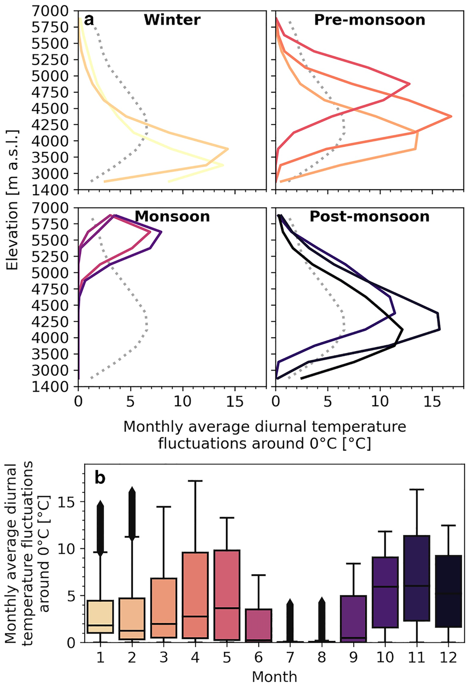
Fig. 3. Monthly average diurnal temperature fluctuations around the freezing point: (a) boxplots and (b) distribution by elevation band averaged over the periods July 2012–June 2014 and July 2016–June 2019. The dotted gray line indicates the annual average distribution.
Table 3. Diurnal temperature fluctuations around the freezing point at the stations

3.1.2 Precipitation
The annual cumulative precipitation at AWS Kyangjin is 798 mm, averaged over the periods July 2012–June 2014 and July 2016–June 2019, which agrees with other meteorological observations (Upreti and others, Reference Upreti2017). The seasonal variability is similar as observed in other studies, with (i) most frequent events and most precipitation in the monsoon season, (ii) more extreme but less events in winter and (iii) less precipitation in pre- and post-monsoon seasons (Bookhagen and Burbank, Reference Bookhagen and Burbank2010; Immerzeel and others, Reference Immerzeel, Petersen, Ragettli and Pellicciotti2014).
As we use the spatial pattern of WRF simulations to extrapolate observed precipitation according to the ratios, we compare the simulated against observed precipitation ratios to AWS Kyangjin for the stations (Fig. 4). The simulated ratios agree reasonably well with the observed ratios (RMSE = 0.55), which indicates that the WRF simulations give a plausible spatial distribution of the precipitation. In November and December the cumulative precipitation is negligible with only 0.8 and 1.3 mm w.e. at AWS Kyangjin, respectively, which easily results in high ratios and large relative differences. Without November and December the RMSE reduces to 0.4. The model tends to overestimate the precipitation ratios, which can partly be explained by the lack of undercatch correction at Pluvio Yala and Pluvio Morimoto. On the contrary, Bonekamp and others (Reference Bonekamp, Collier and Immerzeel2018) found that WRF tend to overestimate summer precipitation below 4600 m a.s.l., and underestimate above 4600 m a.s.l., which may lead to underestimated simulated ratios. The spatial precipitation patterns agree with previous findings based on WRF simulations, with peak values found to be around 3000 m a.s.l. where the topography blocks the large-scale winds during the monsoon, and above 5000 m a.s.l. in the non-monsoon seasons (Collier and Immerzeel, Reference Collier and Immerzeel2015). The increase in precipitation with elevation above 3862 m a.s.l. is also in line with meteorological observations in the catchment (Seko, Reference Seko1987; Fujita and others, Reference Fujita, Sakai and Chhetri1997; Baral and others, Reference Baral2014).

Fig. 4. Simulated against observed monthly precipitation ratios to AWS Kyangjin. Circles indicate Pluvio Langshisha, plusses Pluvio Yala, triangles AWS Yala BC and crosses Pluvio Morimoto.
The annual catchment average precipitation is 1520 mm w.e., of which 500 mm w.e. (33%) falls as snow, falls within the range of previous findings of 17 and 42% (Immerzeel and others, Reference Immerzeel, Petersen, Ragettli and Pellicciotti2014; Bonekamp and others, Reference Bonekamp, de Kok, Collier and Immerzeel2019). In total, 73% of the precipitation falls during the monsoon, which also agrees with findings of Immerzeel and others (Reference Immerzeel, Petersen, Ragettli and Pellicciotti2014). This monsoonal precipitation constitutes 28% of the total snowfall and 95% of the total rainfall.
3.1.3 Incoming shortwave radiation
Figure 5 shows the monthly average diurnal cycle of observed and simulated incoming shortwave radiation and the simulated clear-sky incoming shortwave radiation. The model captures the seasonal pattern reasonably well, with least incoming shortwave radiation during the monsoon season. This is related to cloud cover and agrees with previous studies (Adhikari, Reference Adhikari2012; de Kok and others, Reference de Kok2020). However, the model generally slightly overestimates the amount of incoming radiation, which is most pronounced AWS Yala Glacier, the highest station. This disagreement is related to underestimated atmospheric transmissivity due to a deficit of clouds and atmospheric moisture, which increases with elevation (Orr and others, Reference Orr2017; Bonekamp and others, Reference Bonekamp, Collier and Immerzeel2018), which may lead to overestimated melt at higher elevations. The peak values of the clear-sky radiation at the AWSs are close to the solar constant of 1362 W m−2. This can be attributed to the high elevation and low latitude, and therefore negligible attenuation of radiation within the atmosphere (Adhikari, Reference Adhikari2012). The difference between clear-sky radiation and net radiation is relatively large, emphasizing the importance to correct for transmissivity.

Fig. 5. Simulated (clear-sky) and observed monthly diurnal cycle of incoming shortwave radiation at the stations.
Since the maximum solar elevation angle during the monsoon is 89°, the incoming shortwave radiation during the monsoon is quite evenly distributed in the catchment. During the winter the maximum solar elevation angle is 53° and south-facing slopes therefore receive on average most and north-facing slopes receive least radiation, which enhances melt processes at south-facing slopes compared to north-facing slopes. West-facing and east-facing slopes receive a similar amount of incoming shortwave radiation, with west-facing slopes receiving most radiation in the afternoon and east-facing slopes in the morning. Temperatures in the afternoon are generally higher than those in the morning, which is expected to enhance melt processes at west-facing slopes compared to east-facing slopes.
3.2 Melt parameter estimation
The melt parameter values, estimated from observed ablation time series are T m = −3°C, F t = 0.127 mm w.e. h−1 °C−1 and F sr = 0.00393 mm w.e. h−1 °C−1. The F t and F sr are higher than the values of Saloranta and others (Reference Saloranta2019) (0.11 and 0.0029 mm w.e. h−1 °C−1, respectively), which were based on clear-sky incoming shortwave radiation.
3.3 Model validation
The model outputs were validated against in situ snow depth and SWE observations (Fig. 6). The model captures the seasonal inter-annual and spatial variability of the snow depth and SWE. The simulated melt onset is occasionally a few days to weeks earlier, especially in 2017 and 2018, which we expect to be related to the relative dryness of those years, as less regular snowfall events could result in low albedos. At Pluvio Langshisha, the SWE is somewhat overestimated, which might be related to overestimated snowfall. In addition, the simulated snow cover extent was validated against the MOD10A2 snow cover product (Fig. 14; Appendix A). The simulated and observed snow cover extent during the non-monsoon seasons are in moderate agreement (RMSE = 20%). During the winter and pre-monsoon the simulated snow cover extent generally shows a good match with the observed snow cover extent. The performance is lowest during the post-monsoon (RMSE = 25%) and around 5000 m a.s.l., with the model underestimating the snow cover extent. This is in line with the snow depth validation of AWS Yala BC during the post-monsoon season of 2013, and might be related to uncertainty in lapse rates in this season and/or overestimated incoming shortwave radiation at high elevations (Figs 2 and 5). However, the poorest performance is found in areas with complex topography (Fig. 14b), which suggests that the discrepancy can partly be attributed to the coarse resolution of MODIS (500 m) that does not represent the complex topography of the catchment. The simulations show in general a reasonable agreement with the multiple observations and the RMSE values are relatively low, indicating a good model performance.
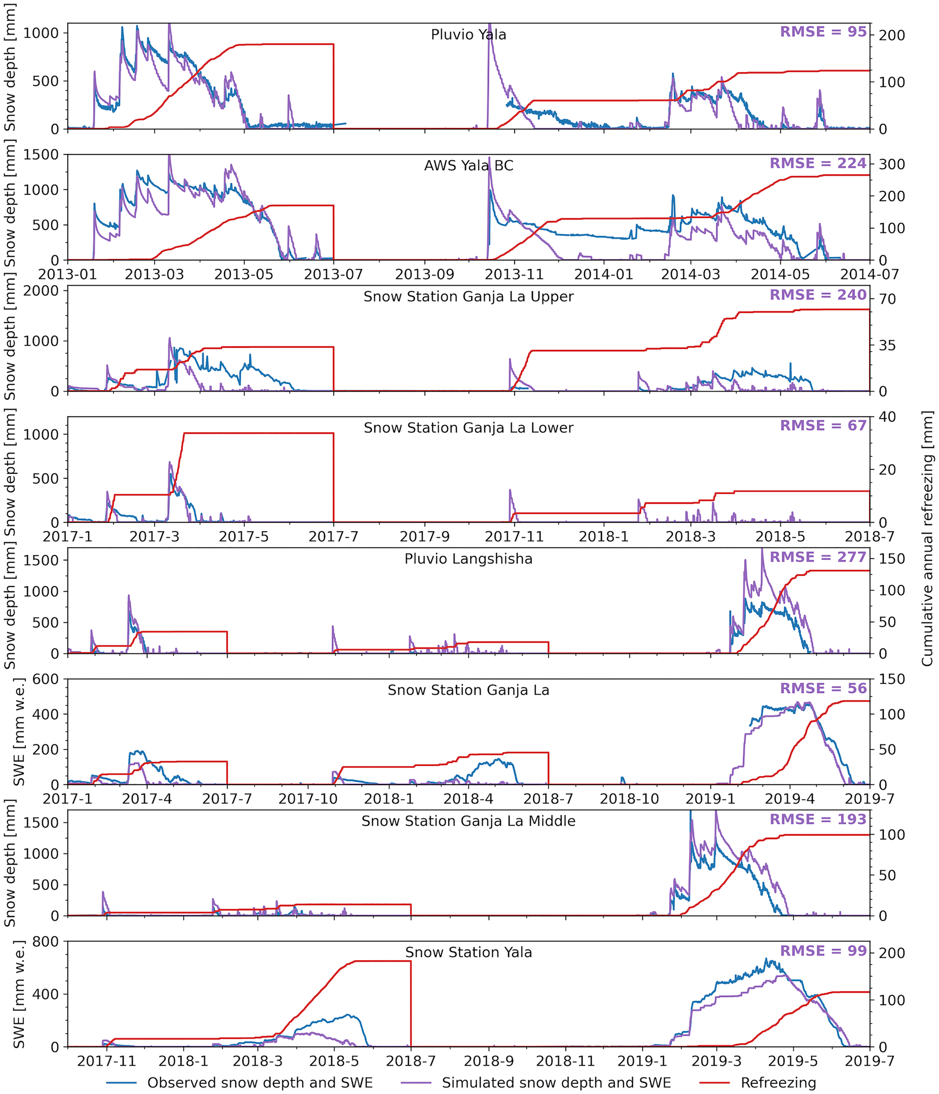
Fig. 6. Simulated and observed snow depth and SWE at stations for periods with measurements, including the simulated cumulative annual refreezing at the stations.
3.4 Spatial-refreezing patterns
Figures 7a–c show spatial maps of the annual average refreezing and refreezing melt ratio, and the annual average refreezing, melt, rain and refreezing melt ratio distribution by elevation band. Refreezing generally increase with elevation, and the refreezing melt ratio also generally increases with elevation, however with a distinct minimum in the 5250–5750 m a.s.l. elevation bands. The increase of refreezing and refreezing melt ratio with elevation can largely be explained by decreasing temperatures and increasing snowfall, and therefore increasing SWE with elevation. The refreezing melt ratio minimum can be explained by the larger insulating effect of thicker snowpacks compared to thinner snowpacks at lower elevation, which limits the increase in refreezing with elevation, and by lower and/or less frequent diurnal temperature fluctuations around the freezing point at this elevation (Fig. 3). The maximum amount of refreezing is 509 mm w.e. (38% of the melt) and occurs at 5850 m a.s.l. Melt increases with elevation until the 5500–5750 m a.s.l. elevation band, whereas rain increases with decreasing elevation until the 3000–3500 m a.s.l. elevation band, which can be explained by decreasing air temperature with elevation and altitudinal differences in precipitation. The annual catchment average refreezing is 122 mm w.e. (21% of the total melt), which is equivalent to 24% of the annual catchment average snow accumulation.
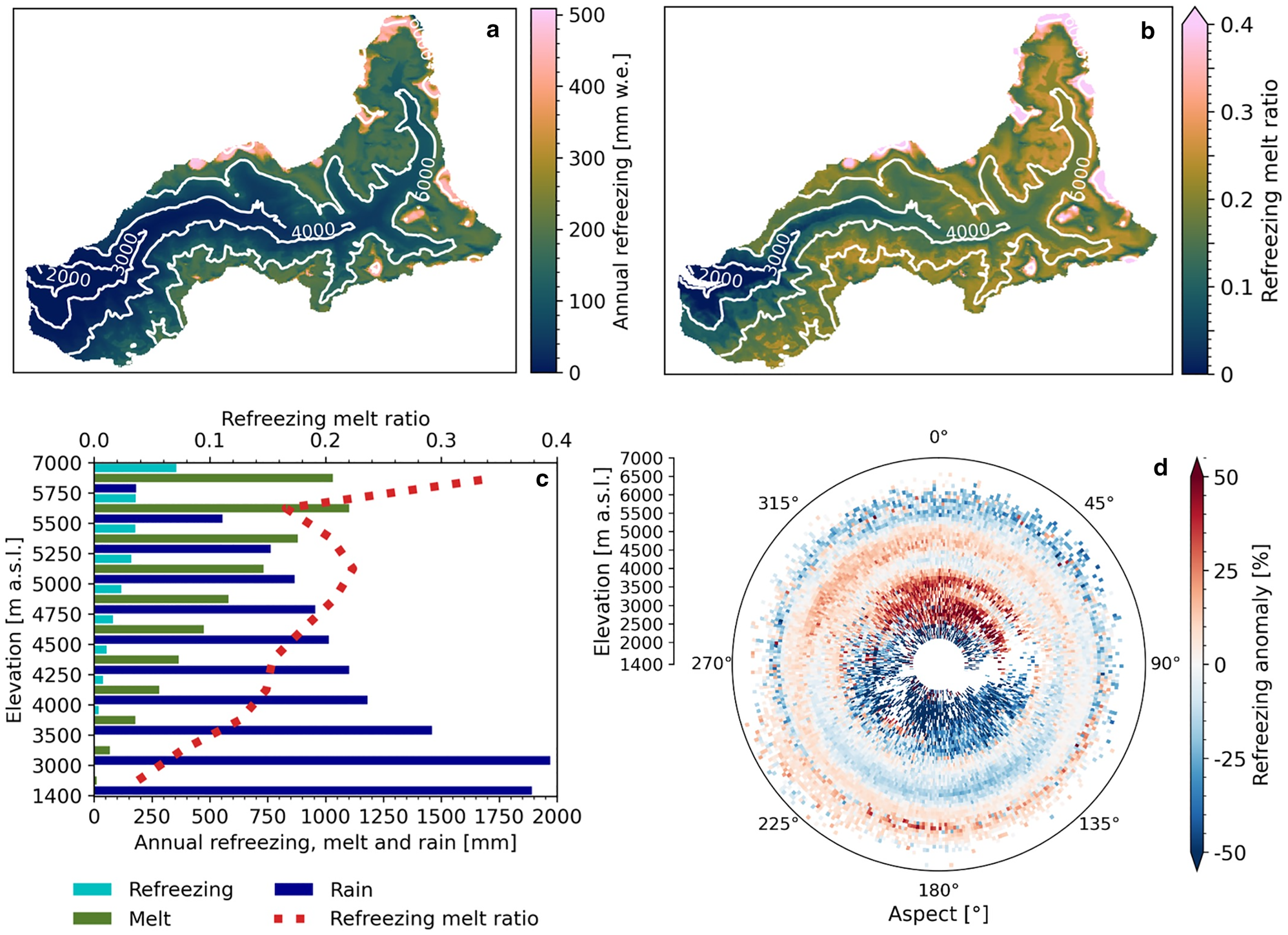
Fig. 7. Annual average (a) refreezing spatial pattern, (b) refreezing melt ratio spatial pattern, (c) refreezing, melt, rain and refreezing melt ratio distribution by elevation band and (d) refreezing anomaly distribution by aspect calculated against the averages of 100-m bins, averaged over the periods July 2012–June 2014 and July 2016–June 2019.
The relative refreezing anomaly distribution by aspect, calculated against the averages of 100-m elevation bins, is shown in Fig. 7d. This figure reveals that below 5250 m a.s.l. refreezing is higher on north-facing than that on other slopes at an equal elevation, while above 5250 m a.s.l. refreezing is highest on south-facing slopes. The average refreezing anomaly on north-facing slopes (315–345°) below 5250 m a.s.l. is 14% and the average refreezing anomaly on south-facing slopes (135–225°) above 5250 m a.s.l. is 8%. This pattern can be explained by differences in shortwave radiation, as south-facing slopes receive more radiation than north-facing slopes, which increases melt. This suggests that at higher elevations thicker snowpacks can store the additionally generated meltwater, which increases melt–refreeze cycles. At lower elevations, the additionally generated meltwater results in a quicker depletion of the snowpack.
3.5 Temporal refreezing patterns
The annual average cycles of refreezing, melt, rain and the refreezing melt ratio are shown in Fig. 8. Refreezing has a strong seasonality, and is most significant in the non-monsoon seasons, during which 38% of the melt (120 mm) refreezes, compared to 21% (122 mm) during the complete year. Refreezing is most substantial during the pre-monsoon season, as this is at the end of the accumulation season, and thus high amounts of snow are present, in combination with strong diurnal temperature fluctuations around the freezing point (Fig. 3a). This is followed by the post-monsoon season, when lower amounts of SWE limit refreezing. However, the refreezing melt ratio is highest from November to February, as there is limited melt. During the monsoon season there is negligible refreezing, with only 3% of the melt that refreezes (2 mm), as the diurnal temperature variability is very low (Fig. 2).

Fig. 8. Monthly catchment average refreezing, melt, rain and refreezing melt ratio averaged over the periods July 2012–June 2014 and July 2016–June 2019.
The seasonal distribution of refreezing, melt, rain and refreezing melt ratio by elevation band is shown in Fig. 9. During the winter refreezing predominantly occurs at relative low elevation. The refreezing distribution shifts upward in the course of the pre-monsoon and monsoon seasons. During the post-monsoon season, the refreezing distribution shifts downward again. Although the temperature conditions during the pre- and post-monsoon seasons are comparable, lower amounts of SWE in the post-monsoon season result in considerably less refreezing below 5500 m a.s.l. During the post-monsoon and winter seasons, refreezing exceeds melt above 5750 m a.s.l., which can be attributed to refreezing of previously stored water, predominantly generated during the monsoon. However, as our model does not include refreezing of meltwater which percolates in a cold deep snowpack, refreezing during monsoon at high elevation might be underestimated, which may result in overestimated storage of meltwater within the snowpack and therefore overestimated refreezing during the post-monsoon. Refreezing is most substantial during the pre-monsoon, with a maximum of 40 mm w.e. month−1 (40% of the melt) in the 5250–5500 m a.s.l. elevation band.
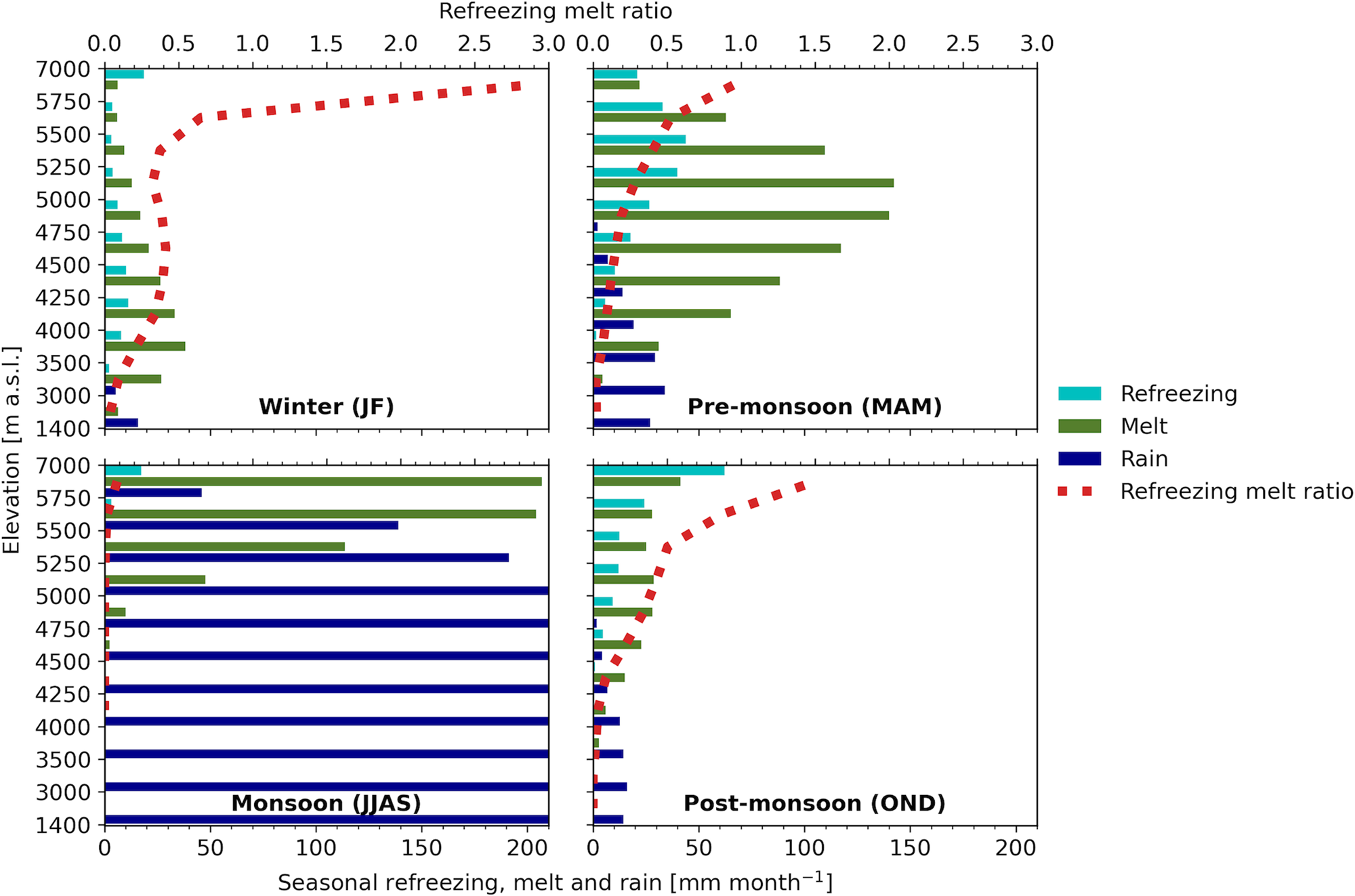
Fig. 9. Seasonal average refreezing, melt, rain and refreezing melt ratio distribution by elevation band averaged over the periods July 2012–June 2014 and July 2016–June 2019.
Time series elevation profiles of monthly refreezing, average SWE, average diurnal temperature fluctuations around the freezing point and snowfall are shown in Fig. 10. The aim of this figure is to show how monthly altitudinal refreezing patterns differs between years and to identify the controlling factors. As an indication of the average monthly temperature, the zero degree isotherm is also shown. The lack of snow redistribution and sublimation results in increasing accumulation above 5800 m a.s.l. Hence, we focus on the output below 5800 m a.s.l. Large inter-annual variability is found from January to March, during which large amounts refreezing occur below 5000 m a.s.l. in 2013 and 2019 compared to other years (Fig. 10a). This is related to high amounts of SWE caused by snowfall, in combination with relatively low temperatures (Figs 10b–d). The inter-annual differences in the post-monsoon season are also large, with high amounts of refreezing in 2013, related to high average SWE caused by a snowstorm in October, while the temperatures in the post-monsoon are relatively consistent. The inter-annual variability during the monsoon is low, as the snowfall and temperature are relatively consistent. The annual catchment average refreezing varies between 163 mm w.e. (24% of melt) in 2013–14 and 102 mm w.e. (23% of melt) in 2017–18. The refreezing melt ratio varies between 0.19 in 2012–13 and 0.24 in 2013–14.

Fig. 10. Monthly time series elevation profiles of (a) refreezing, (b) average SWE, (c) snowfall and (d) average diurnal cumulative hourly temperature fluctuations around the freezing point averaged over 100-m elevation bins. The black line indicates the monthly average zero degree isotherm elevation.
We investigated the importance of using sub-daily time steps to capture melt–refreeze cycles, by comparing the hourly refreezing simulation with the daily simulation. The annual catchment average refreezing of the daily simulations is 19 mm w.e. (−84%) and the melt is 391 mm w.e. (−32%), which results in a refreezing melt ratio of 0.05 compared to 0.21 of the hourly simulation. The decrease in melt results in a later melt onset of several days to weeks depending on elevation, with ~2 weeks at the median elevation of 4900 m a.s.l. In addition, we found that 93 mm w.e. (76%) of the melt that refreezes, was generated within the previous 24 h.
3.6 Sensitivity analysis
We investigated the effects of uncertainties in meteorological forcing, albedo and the melt parameters on our final results. The resulting std dev. of the output, a measure of the sensitivity, for refreezing is 14 mm w.e. (11% of the reference), for the refreezing melt ratio 0.03 (14% of the reference) and for melt 62 mm w.e. (11% of the reference). The independent refreezing and refreezing melt ratio sensitivities to different inputs and parameters are presented in Appendix B.
The refreezing, refreezing melt ratio and snowfall sensitivities to potential changes in air temperature and precipitation as a function of deviation from the mean (0% scenario) are shown in Fig. 11. The corresponding elevation sensitivity profiles of refreezing and the refreezing melt ratio are shown in Fig. 12. The refreezing profile shifts linearly upward with increasing temperature, and downward with decreasing temperature (Fig. 12a). This results in decreasing and increasing refreezing, respectively, as the surface area decreases with elevation within this range (Fig. 1c). However, the refreezing amounts respond non-linearly to changes in temperature, with a stronger increase in refreezing than decrease. The refreezing melt ratio profile shows a similar response, with decreasing ratios with increasing temperature (Fig. 12d). Clearly, refreezing and the refreezing melt ratio are considerably less sensitive to the precipitation changes (Figs 12b, e). This is also illustrated by the significantly stronger control of the variable temperature than the variable precipitation on snowfall (Fig. 11c). Refreezing increases with increasing precipitation, while the refreezing melt ratio decreases with increasing precipitation. Again, we find a non-linear response, with a higher sensitivity to decreasing than increasing precipitation. The refreezing and refreezing melt ratio sensitivities to the simultaneously changed temperature and precipitation show that the variable precipitation alters the temperature impact in only a very limited way (Figs 12c, f). This is as expected, since the sensitivity to the precipitation changes is substantially lower.

Fig. 11. Annual catchment average (a) refreezing, (b) refreezing melt ratio and (c) snowfall with respect to potential changes in air temperature and precipitation averaged over the periods July 2012–June 2014 and July 2016–June 2019.

Fig. 12. Elevation profiles of refreezing (top row) and refreezing melt ratio (bottom row) with potential changes in (a, d) air temperature, (b, e) precipitation and (c, f) air temperature and precipitation, averaged over 10-m elevation bins and over the periods July 2012–June 2014 and July 2016–June 2019. The left panel of each subplot shows the simulated refreezing and refreezing melt ratio and the right panel of each subplot shows the difference between the perturbated run and the reference run (the sensitivity). The yellow line indicates the reference run.
Figure 13 shows the time series of the refreezing and refreezing melt ratio with variable temperature and precipitation. The sensitivity to the temperature changes has a strong seasonality, with the highest refreezing sensitivity in the post-monsoon followed by the pre-monsoon season (Fig. 13a). The temperature changes cause a shift in the pre-monsoon season, with earlier refreezing with increasing temperatures, related to an earlier melt onset. The melt ratio sensitivity is most pronounced in the winter season, which is related to low amounts of melt, resulting in high and easily changed ratios. The highest refreezing sensitivity to the variable precipitation is observed during the pre- and post-monsoon seasons. This is as expected, since snowfall during the post-monsoon and pre-monsoon often melts within the same season, while snowfall in winter season generally gets stored over the pre-monsoon season. The refreezing sensitivity to temperature and precipitation changes shows a modest inter-annual variability, with the lowest sensitivities in the pre-monsoon of 2013 and 2019 and the post-monsoon of 2013, which are melting periods characterized by high amounts of SWE (Fig. 10b).
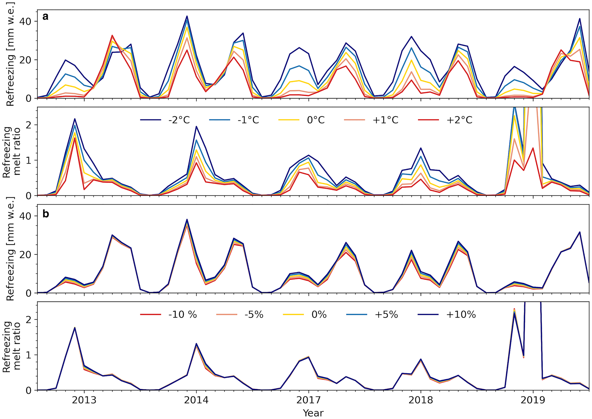
Fig. 13. Monthly time series of refreezing and the refreezing melt ratio with variable (a) temperature and (b) precipitation. The yellow line indicates the reference run.
4. Discussion
4.1 Model performance
In general, we observe a good correspondence between the simulated and observed snow depth, SWE and snow cover extent (Figs 6 and 14). This indicates that the seNorge snow model is capable of capturing the seasonal snow dynamics. In addition, the validation results are comparable to other studies in the catchment (Stigter and others, Reference Stigter2017; Saloranta and others, Reference Saloranta2019). However, the validation results show that the simulated melt onset is too early in 2017 and 2018 (Fig. 6). The melt onset is captured relatively well during the other years, when deeper snowpacks occur. Therefore, we expect that this might be related to the relative dryness of those years, as less regular snowfall events could result in low albedos. The validation results also reveal that the model underestimates snow depth and snow cover in the post-monsoon season. This could be related to uncertainty in lapse rates in this season and/or overestimated incoming shortwave radiation at high elevations (Figs 2 and 5). The low correlation of the lapse rates is likely caused by the large inter-annual variability in snowfall events and snow cover during this season (Heynen and others, Reference Heynen2016). As snow cover has a cooling effect due to increased albedo, the lapse rates during snow covered years are likely steeper, explaining the disagreement (Kattel and others, Reference Kattel2013). Calculating lapse rates for each year separately during the post-monsoon could overcome this problem; however, this would result in less robust lapse rates in periods with few observations.
Our refreezing and refreezing melt ratio estimates agree with previously established values in the catchment. The simulated catchment average refreezing of 122 mm w.e. a−1 and the refreezing melt ratio of 0.21 during the complete year and 0.38 during the non-monsoon seasons are in agreement with Saloranta and others (Reference Saloranta2019), who estimated that 36% of the melt refreezes during the complete year and 48% during the non-monsoon seasons. The modest discrepancy could be related to their use of average daily lapse rates and clear-sky incoming shortwave radiation, and to inter-annual variability. Figure 2 clearly shows that the lapse rates are shallower during the night and steeper during the day. The use of daily average lapse rates therefore results in underestimated temperatures during the night and overestimated temperatures during the day, at higher elevation than from where is extrapolated (4200 m a.s.l.). This is where refreezing predominantly occurs and the overestimated favorable conditions, could explain the disagreement. This confirms the importance of using sub-daily lapse rates in snow models. The use of clear-sky incoming shortwave is likely also favorable for refreezing, as radiation generates meltwater at close to zero temperatures, which potentially refreezes (Bookhagen and Burbank, Reference Bookhagen and Burbank2010; Matthews and others, Reference Matthews2020). Saloranta and others (Reference Saloranta2019) found at Snow Station Ganja La that 34% of the melt refreezes. Stigter and others (Reference Stigter2021) found at Snow Station Ganja La that 32% of the melt refreezes and at AWS Yala BC 34% using a point-scale energy-balance model. In addition, Stigter and others (Reference Stigter2021) observed ice layers and a melt–freeze crust, which develop by refreezing of meltwater, with a total thickness of 56–81 mm at Snow Station Yala, and Kirkham and others (Reference Kirkham2019) observed ice layers with a total thickness of 60–140 mm at Snow Station Ganja La.
Diurnal melt–refreeze cycles during the melt season are also observed by radar remote sensing in the Karakoram (Lund and others, Reference Lund2020). Although remote-sensing products provide no information about refreezing quantities and driving processes, they can be used to confirm melt–refreeze cycles and also to validate wet and dry snowpacks. Their results suggests that diurnal melt–refreeze cycles predominantly occur in the early melt season, during which the median elevation of melt–refreeze cycles increases and during which intra-annual differences in extent and onset occur. These results are in line with our findings. Figure 9 shows a considerable amount of rainfall and melt at high elevation (>5750 m a.s.l.) during the monsoon. This meltwater is partly stored within the snowpack and refreezes during the post-monsoon and winter, where refreezing exceeds the melt estimates. However, remote-sensing products show dry snowpacks, especially at high elevations, outside the melt season in the High Mountain Asia (Snapir and others, Reference Snapir, Momblanch, Jain, Waine and Holman2019; Lund and others, Reference Lund2020). The overestimated wetness can be explained by the fact that our model does not include refreezing of meltwater which percolates in a cold deep snowpack, which is especially important for thick snowpacks at high elevations. This indicates that our refreezing simulations above 5750 m a.s.l. are delayed. In addition, as explained in Section 3.1, temperature and incoming shortwave radiation might be overestimated at high elevations, which may result in overestimated melt.
Studies from other regions focus solely on refreezing on glacier surfaces, which has implications for local forcing of melt, from the surface as well as the base of the snowpack. However, our estimates fall well within previously established fractions in different climatic environments. Samimi and Marshall (Reference Samimi and Marshall2017) estimated that 10% of a supraglacial snowpack in the Canadian Rocky mountains refreezes. Mölg and others (Reference Mölg, Maussion, Yang and Scherer2012) and Fujita and Ageta (Reference Fujita and Ageta2000) estimated that 13 and 20% of the snowmelt refreezes, respectively, on two glaciers on the Tibetan Plateau, using an energy-balance model.
4.2 Refreezing patterns
The catchment average refreezing of 122 mm w.e. a−1 (21% of the melt) shows that significant amounts of meltwater refreeze in the catchment. The two prerequisites for refreezing are availability of meltwater and below zero temperatures within the snowpack. The primary drivers of the spatial pattern of the model output are therefore the amount of snow, which is required to generate and store meltwater, and the magnitude and frequency of temperature fluctuations around the freezing point, which is required to generate and subsequently refreeze meltwater. In addition, incoming shortwave radiation is also an important driver of the model output, as it generates significant melt at close to zero temperatures, which can subsequently refreeze (Bookhagen and Burbank, Reference Bookhagen and Burbank2010; Matthews and others, Reference Matthews2020). As air temperature and amount of snow are strongly correlated with elevation, refreezing and the refreezing melt ratio also have a strong relation with elevation. Refreezing generally increases with elevation up to 5900 m a.s.l., indicating that meltwater availability limits refreezing above this elevation. The refreezing melt ratio also generally increases with elevation, with a minimum in the 5250–5750 m a.s.l. elevation band (Fig. 7c). This minimum can be explained in two ways: (i) the snowpack predominantly melts during the monsoon, during which diurnal temperature fluctuations are small, resulting in a rapid SWE decrease and (ii) the deep snowpack has a large insulating effect, which limits the increase in refreezing with elevation. The insulating effect is supported by findings of Lund and others (Reference Lund2020), as snowpacks which are wet both day and night are observed at a higher elevation than snowpacks which are wet during the day and dry during the night.
Besides the altitudinal refreezing pattern, we also found a pattern related to aspect. Figure 7d reveals that below 5250 m a.s.l. refreezing is significantly higher (14%) on north-facing slopes, while above 5250 m a.s.l. refreezing is significantly higher (8%) on south-facing slopes. This is related to higher incoming shortwave radiation at south-facing than at north-facing slopes, which generates additional melt. Below 5250 m a.s.l. snowpacks are too shallow to store the generated melt and increased shortwave radiation therefore this accelerates the depletion of the snowpack, which decreases the potential for refreezing. Above 5250 m a.s.l. deeper snowpacks can store the additionally generated meltwater, which increases melt–refreeze cycles. This indicates that it is important to account for incoming shortwave radiation, when quantifying refreezing.
Refreezing has a strong seasonality, and is most substantial during the pre-monsoon season, followed by the post-monsoon season. Temperature fluctuations around the freezing point are stronger in the post-monsoon season, but shallow or absent snowpacks limit refreezing (Fig. 8). The refreezing melt ratio is higher during the post-monsoon season. This can be explained by refreezing of meltwater above 5750 m a.s.l. generated during the monsoon. However, as explained before, refreezing during monsoon at high elevation might be underestimated, which could result in overestimated refreezing in the post-monsoon season due to overestimated storage of meltwater within the snowpack. The higher refreezing melt ratios in the non-monsoon seasons are in agreement with Saloranta and others (Reference Saloranta2019), who estimated that 36% of the melt refreezes during the complete year and 48% during the non-monsoon seasons.
Intra-annual differences in refreezing are primarily caused by fluctuations in snowfall, especially during the post-monsoon and pre-monsoon, which result in more SWE accumulation. This is particularly evident for the high amount of snowfall during the post-monsoon season of 2013. Monthly average temperature and diurnal temperature fluctuations around the freezing point have a lower inter-annual variability, which is in line with previous observations (Stigter and others, Reference Stigter2017) and generally show a less clear relation with refreezing. This agrees with other studies, who found that there is a substantial inter-annual variability of snow dynamics in the Langtang catchment, which is predominantly controlled by the large inter-annual variability of snowfall (Seko and Takahashi, Reference Seko and Takahashi1991; Girona-Mata and others, Reference Girona-Mata, Miles, Ragettli and Pellicciotti2019). The large inter-annual differences in refreezing emphasize the importance of multi-year time series in refreezing assessments. The less clear relation with temperature compared to precipitation is opposite to the sensitivity analysis results, which can be explained by the considerable larger inter-annual fluctuations than the sensitivity analysis changes for precipitation.
The substantial decrease in refreezing to 19 mm w.e. (−84%) with the daily time step highlights the importance of using sub-daily time steps to capture melt–refreeze cycles. This is supported by the large amount of temperature fluctuations around the freezing point (Fig. 3 and Table 3).
4.3 Sensitivity analysis
The meteorological forcing and albedo sensitivity analysis shows that our estimates for refreezing and refreezing melt ratio are robust, as we estimate std dev.s of 8.5 and 9.2%, respectively. This supports the conclusions drawn in this study. However, we have only focused on the lapse rate, precipitation, incoming shortwave radiation and albedo, but other variables, such as the rain-snow temperature threshold, might add significant uncertainty (Jennings and others, Reference Jennings, Winchell, Livneh and Molotch2018). In addition, due to computational restrictions we only performed 200 realizations.
The climate sensitivity analysis reveals that refreezing is very sensitive to variable temperature, as a temperature increase of 2°C leads to a refreezing decrease of 35%. This is caused by less snow accumulation, a shorter snow season and less diurnal temperature fluctuations around the freezing point. In comparison, refreezing is less sensitive to variable precipitation, since air temperature exerts a strong control on snowfall, illustrated by the fact that a 2°C temperature increase results in a snowfall decrease of 35%. Therefore, the 10% precipitation increase compensates the effects of the 2°C temperature increase only to a limited degree. However, this also indicates that refreezing is sensitive to variable snowfall with variable temperature as the driver. The relatively low sensitivity to variable temperature and precipitation during years with high amounts of snowfall reveals that snow has a buffering effect, while during relatively warm and dry years, the model is more sensitive.
4.4 Model limitations and recommendations for future research
Several limitations of this study should be noted, which may be improved in future research. One limitation of our model is that we do not include longwave radiation and turbulent fluxes, as these are not always well correlated with air temperature and incoming shortwave radiation this may impact melt–refreeze cycles (Ayala and others, Reference Ayala, Pellicciotti, MacDonell, McPhee and Burlando2017b; Litt and others, Reference Litt2019). In addition, Stigter and others (Reference Stigter2021) show that 21% of the positive net energy during the day is used to overcome the nightly increase in cold content around 5000 m a.s.l. in Langtang area. In line with this, our model does not include refreezing of meltwater which percolates in a cold deep snowpack. Including the cold content in our model would likely improve our understanding about melt–refreeze cycles. In addition, our model assumes that meltwater immediately infiltrates and gets distributed evenly throughout the snowpack. However, water percolates with a speed of 1–10 mm h−1 in an isothermal snowpack (Samimi and Marshall, Reference Samimi and Marshall2017). This could be included with the common bucket approach (Verjans and others, Reference Verjans2019). Another simplification is that we do not differentiate between rain and snowmelt refreezing, while part of the water retained within snowpacks originates from rainfall. However, Kirkham and others (Reference Kirkham2019) observed around 5000 m a.s.l. in Langtang area, that only very little of the SWE accumulation originates from rainfall. Additionally, since the model is a simplified one-layer model, this study has not attempted to address the formation of water lenses. A significant part of the catchment is glacierized (Fig. 1b), which has implications for local energy forcing from the surface and the base of snowpacks, therefore future research could focus on differences of refreezing in supraglacial snowpacks.
We have compared our refreezing estimates with ice layer measurements of Kirkham and others (Reference Kirkham2019) and Stigter and others (Reference Stigter2021). To further validate the refreezing algorithm, we suggest validating simulated refreezing on a point-scale forced with meteorological observations. Refreezing can be measured with multiple temperature measurements at different depths in the snowpack to obtain temperature profiles (Wright and others, Reference Wright2007; Stigter and others, Reference Stigter2021), or with time-domain reflectometry probes, which measure snow water content (Samimi and Marshall, Reference Samimi and Marshall2017) or by measuring ice layers within a snow pit.
The refreezing estimates of this study are comparable or higher compared to other delays or energy deficits, such as subsurface flow (Andermann and others, Reference Andermann2012; Pradhananga and others, Reference Pradhananga2014) and wind transport (Bernhardt and others, Reference Bernhardt, Schulz, Liston and Zängl2012), and loss terms such as sublimation (Stigter and others, Reference Stigter2018). This indicates that refreezing is a significant component of the water balance and that is important to include when simulating snowpack persistence and snowmelt runoff timing in Himalayan catchments. Including refreezing may therefore be especially important for flood forecasting, and reservoir and hydropower operations optimization.
5. Conclusion
In this study, we simulated refreezing with the seNorge (v2.0) snow model, which has an analytical refreezing algorithm, for the Langtang catchment in the Nepalese Himalaya covering a 5-year period. Thereby, the aim was to improve our understanding about how refreezing varies in space and time. To optimize the model performance, the meteorological forcing data were derived from a unique elaborate network of meteorological stations and high-resolution WRF simulations. The frequent diurnal temperature fluctuations around the freezing point suggest that the conditions are favorable for refreezing. In general, the simulations show a reasonable agreement with in situ snow observations and remotely sensed snow cover data, indicating a good model performance.
The catchment average refreezing of 122 mm w.e. a−1 (21% of the total melt) shows that significant amounts of meltwater refreeze in the catchment. We found that the magnitudes of refreezing and the refreezing melt ratio vary substantially in space, with a strong relation with elevation, related to diurnal temperature fluctuations around the freezing point and snow depth. Refreezing also has a spatial pattern related to aspect, caused by differences in incoming shortwave radiation. The average refreezing anomaly on north-facing slopes below 5250 m a.s.l. is 14% and the average refreezing anomaly on south-facing slopes above 5250 m a.s.l. is 8%. This shows that it is important to account for incoming shortwave radiation when quantifying refreezing. In addition, there is a strong seasonal altitudinal variability related to temperature fluctuations around the freezing point and snow depth, with most refreezing during the non-monsoon seasons (38% of the melt). Most refreezing occurs during the pre-monsoon season, with a maximum of 40 mm w.e. month−1 (40% of the melt) in the 5250–5500 m a.s.l. elevation band. During the monsoon season there is negligible refreezing, with only 3% of the melt that refreezes (2 mm w.e.), as the temperatures are constant throughout the day.
We also found a substantial intra-annual variability, which mainly results from fluctuations in post-monsoon and winter snowfall, highlighting the importance of using multi-year time series in refreezing assessments. Daily refreezing simulations decreased by 84% (to a catchment average of 19 mm w.e. a−1) compared to hourly simulations, emphasizing the importance of using sub-daily time steps to capture diurnal melt–refreeze cycles. The meteorological forcing and albedo sensitivity analysis shows that our estimates for refreezing and the refreezing melt ratio are robust, as the resulting std dev.s are 8.5 and 9.2%, respectively. Climate sensitivity experiments revealed that refreezing is highly sensitive to changes in air temperature and thereby snowfall, as a temperature increase of 2°C leads to a refreezing decrease of 35%. We conclude that including distributed refreezing with a sub-daily temporal resolution is highly relevant for understanding snow dynamics in the current and future climate of the Himalaya.
Acknowledgements
This study was funded by the European Research Council (Grant Agreement No. 676819) and by the Netherlands Organization for Scientific Research NWO (Grant Agreement No. 016.181.308). This study was also financially funded by ICIMOD's Cryosphere Initiative funded by Norway, and by core funds contributed by the Governments of Afghanistan, Australia, Austria, Bangladesh, Bhutan, China, India, Myanmar, Nepal, Norway, Pakistan, Sweden and Switzerland. We thank the reviewers for thorough and constructive reviews that helped to improve the manuscript.
Author contributions
SV, WI, RK, ES and JS defined the research goals and designed the study. SV developed the meteorological forcing data, performed the model experiments and analyzed the results. TS performed the melt parameters’ estimation analysis. SV wrote the initial version of the manuscript. All authors provided feedback and improved the manuscript.
Appendix A: MODIS validation
See Fig. 14.

Fig. 14. (a) Simulated and observed (MODIS) 8-d maximum snow cover extent for the non-monsoon seasons. (b) Spatial pattern of difference between total simulated and observed (MODIS) 8-d maximum snow cover extent for the period July 2012–June 2014, July 2016–June 2019 for the non-monsoon seasons.
Appendix B: Sensitivity analysis
In order to complement our sensitivity analysis to input and parameter uncertainty, we performed two additional runs for each of the seven variables. We adjusted the values by subtracting and adding the std dev.s (values described in Section 2.6), which resulted in 14 additional runs. The refreezing and refreezing melt ratio sensitivities are listed in Table 4, and the corresponding elevation profiles are shown in Fig. 15. The ensemble means of the Monte Carlo analysis have also been included in Table 4 and Fig. 15. The results show that refreezing is most sensitive to the albedo, lapse rate and precipitation uncertainties, and the refreezing melt ratio is most sensitive to albedo and incoming shortwave radiation uncertainties. However, none of the sensitivities are high. Figure 15 reveals that the model is almost exclusively sensitive above 5500 m a.s.l., which covers 16% of the catchment area (Fig. 1c). These results confirm that are estimates for refreezing and refreezing melt ratio are robust and support the conclusions drawn in this study.
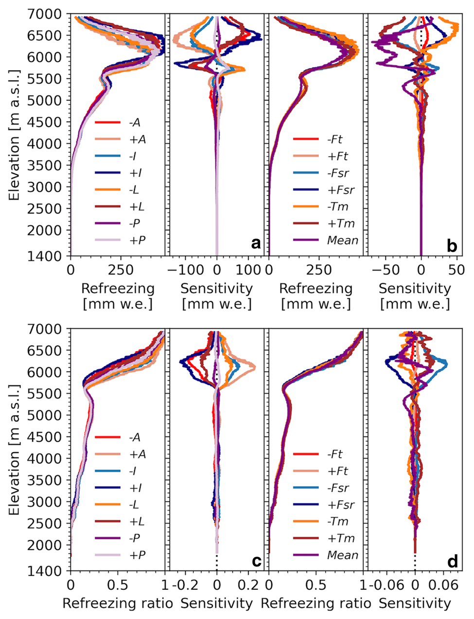
Fig. 15. Elevation profiles of refreezing (top row) and refreezing melt ratio (bottom row) with independently adjusted (a, c) meteorological forcing and albedo and (e, f) melt parameters, averaged over 10-m elevation bins and over the periods July 2012–June 2014 and July 2016–June 2019. The inputs and parameters are changed by subtracting (−) and adding (+) the std dev.s (which are described in Section 2.6). A indicates albedo, I incoming shortwave radiation, L lapse rate, P precipitation, F t temperature melt factor, F sr radiative melt factor, T m threshold for melt onset and Mean the ensemble means of the Monte Carlo analysis. The left panel of each subplot shows the simulated refreezing and refreezing melt ratio and the right panel of each subplot shows the difference between the perturbated run and the reference run (the sensitivity).
Table 4. Overview of annual catchment average refreezing and the refreezing melt ratio with adjusted inputs and parameters


 Open access