


1 Introduction
A process of turbulent thermal convection, which occurs widely in nature, is usually studied in a Rayleigh–Bénard configuration, where a fluid layer is confined between two isothermal horizontal surfaces, a lower warmer one and an upper colder one. In classical Rayleigh–Bénard convection (RBC) (cf. reviews by Ahlers, Grossmann & Lohse (Reference Ahlers, Grossmann and Lohse2009), Lohse & Xia (Reference Lohse and Xia2010) and Chillà & Schumacher (Reference Chillà and Schumacher2012)) the heating and cooling plates are assumed to be smooth, while in most applications this assumption is not fulfilled. Roughness of the heated and cooled plates or the presence of heated and cooled obstacles, which are attached to the corresponding plates, can influence significantly the mean heat and momentum transport in the system, which are represented by the Nusselt number $Nu$
and Reynolds number
$Nu$
and Reynolds number $Re$
, respectively. Moreover, the scaling relations of
$Re$
, respectively. Moreover, the scaling relations of $Nu$
and
$Nu$
and $Re$
on the main input parameters of the system, which are the Rayleigh number
$Re$
on the main input parameters of the system, which are the Rayleigh number $Ra$
and Prandtl number
$Ra$
and Prandtl number $Pr$
, are also affected by the wall roughness.
$Pr$
, are also affected by the wall roughness.
Most of the experimental and numerical studies of RBC in convection cells with rough plates have been conducted for regular roughness, which is determined by a single or only a few roughness scales. These studies generally report an increase of the heat transport compared to the case of smooth plates, as soon as the roughness height becomes comparable to or larger than the boundary-layer thickness in the smooth case. Thus, it was reported in earlier works that, compared to the case of smooth plates, the scaling exponent $\unicode[STIX]{x1D6FE}$
in the scaling relation
$\unicode[STIX]{x1D6FE}$
in the scaling relation $Nu\sim Ra^{\unicode[STIX]{x1D6FE}}$
can be larger (Roche et al.
Reference Roche, Castaing, Chabaud and Herbal2001; Qiu, Xia & Tong Reference Qiu, Xia and Tong2005; Stringano, Pascazio & Verzicco Reference Stringano, Pascazio and Verzicco2006; Tisserand et al.
Reference Tisserand, Creyssels, Gasteuil, Pabiou, Gibert, Castaing and Chillà2011; Salort et al.
Reference Salort, Liot, Rusaouen, Seychelles, Tisserand, Creyssels, Castaing and Chillà2014; Liot et al.
Reference Liot, Salort, Kaiser, du Puits and Chillá2016; Toppaladoddi, Succi & Wettlaufer Reference Toppaladoddi, Succi and Wettlaufer2017; Xie & Xia Reference Xie and Xia2017; Jiang et al.
Reference Jiang, Zhu, Mathai, Verzicco, Lohse and Sun2018) and/or the pre-factor in this relation can be increased (Shen, Xia & Tong Reference Shen, Xia and Tong1996; Du & Tong Reference Du and Tong2000; Wei & Ahlers Reference Wei and Ahlers2014; Joshi et al.
Reference Joshi, Rajaei, Kunnen and Clercx2017).
$Nu\sim Ra^{\unicode[STIX]{x1D6FE}}$
can be larger (Roche et al.
Reference Roche, Castaing, Chabaud and Herbal2001; Qiu, Xia & Tong Reference Qiu, Xia and Tong2005; Stringano, Pascazio & Verzicco Reference Stringano, Pascazio and Verzicco2006; Tisserand et al.
Reference Tisserand, Creyssels, Gasteuil, Pabiou, Gibert, Castaing and Chillà2011; Salort et al.
Reference Salort, Liot, Rusaouen, Seychelles, Tisserand, Creyssels, Castaing and Chillà2014; Liot et al.
Reference Liot, Salort, Kaiser, du Puits and Chillá2016; Toppaladoddi, Succi & Wettlaufer Reference Toppaladoddi, Succi and Wettlaufer2017; Xie & Xia Reference Xie and Xia2017; Jiang et al.
Reference Jiang, Zhu, Mathai, Verzicco, Lohse and Sun2018) and/or the pre-factor in this relation can be increased (Shen, Xia & Tong Reference Shen, Xia and Tong1996; Du & Tong Reference Du and Tong2000; Wei & Ahlers Reference Wei and Ahlers2014; Joshi et al.
Reference Joshi, Rajaei, Kunnen and Clercx2017).
A detailed analysis of the dependences of the scaling exponent $\unicode[STIX]{x1D6FE}$
on
$\unicode[STIX]{x1D6FE}$
on $Ra$
shows that for a fixed configuration of the regular roughness, an increased
$Ra$
shows that for a fixed configuration of the regular roughness, an increased $\unicode[STIX]{x1D6FE}$
is observed only in a certain restricted interval of Rayleigh number. For moderate
$\unicode[STIX]{x1D6FE}$
is observed only in a certain restricted interval of Rayleigh number. For moderate $Ra$
up to
$Ra$
up to $10^{8}$
, the three-dimensional direct numerical simulations (DNS) by Wagner & Shishkina (Reference Wagner and Shishkina2015) in a cubical container with a fixed rectangular roughness showed that the exponent
$10^{8}$
, the three-dimensional direct numerical simulations (DNS) by Wagner & Shishkina (Reference Wagner and Shishkina2015) in a cubical container with a fixed rectangular roughness showed that the exponent $\unicode[STIX]{x1D6FE}$
first increases with growing
$\unicode[STIX]{x1D6FE}$
first increases with growing $Ra$
, but then tends to saturate back to the smooth-wall value. Similar results were obtained using the spectral NEK5000 code in the two-dimensional DNS by Xu et al. (Reference Xu, Wang, Wan, Yan and Sun2018), for a broad
$Ra$
, but then tends to saturate back to the smooth-wall value. Similar results were obtained using the spectral NEK5000 code in the two-dimensional DNS by Xu et al. (Reference Xu, Wang, Wan, Yan and Sun2018), for a broad $Pr$
range and
$Pr$
range and $Ra$
up to
$Ra$
up to $10^{10}$
. Two-dimensional simulations based on the immersed boundary method, which were conducted by Zhu et al. (Reference Zhu, Stevens, Verzicco and Lohse2017) for
$10^{10}$
. Two-dimensional simulations based on the immersed boundary method, which were conducted by Zhu et al. (Reference Zhu, Stevens, Verzicco and Lohse2017) for $Ra$
up to
$Ra$
up to $10^{12}$
, showed that at
$10^{12}$
, showed that at $Ra\approx 3\times 10^{9}$
there exists a well-pronounced change from one scaling regime with
$Ra\approx 3\times 10^{9}$
there exists a well-pronounced change from one scaling regime with $\unicode[STIX]{x1D6FE}\approx 1/2$
for
$\unicode[STIX]{x1D6FE}\approx 1/2$
for $Ra<3\times 10^{9}$
to another regime with
$Ra<3\times 10^{9}$
to another regime with $\unicode[STIX]{x1D6FE}\approx 1/3$
for
$\unicode[STIX]{x1D6FE}\approx 1/3$
for $Ra>3\times 10^{9}$
. Therefore the regime with
$Ra>3\times 10^{9}$
. Therefore the regime with $\unicode[STIX]{x1D6FE}\approx 1/2$
can be interpreted neither as the ultimate regime, which can be expected for extremely high
$\unicode[STIX]{x1D6FE}\approx 1/2$
can be interpreted neither as the ultimate regime, which can be expected for extremely high $Ra$
, nor as a transition to the ultimate regime, but rather as an intermediate regime triggered by the regular roughness. Similar results were obtained also in experiments by Rusaouën et al. (Reference Rusaouën, Liot, Castaing, Salort and Chillà2018) for
$Ra$
, nor as a transition to the ultimate regime, but rather as an intermediate regime triggered by the regular roughness. Similar results were obtained also in experiments by Rusaouën et al. (Reference Rusaouën, Liot, Castaing, Salort and Chillà2018) for $Ra$
up to
$Ra$
up to $10^{12}$
. More precisely, it was found that with increasing
$10^{12}$
. More precisely, it was found that with increasing $Ra$
, the heat transfer first remains unaffected by the plate roughness, then the heat transport is enhanced and this is reflected in an increased
$Ra$
, the heat transfer first remains unaffected by the plate roughness, then the heat transport is enhanced and this is reflected in an increased $\unicode[STIX]{x1D6FE}$
, and finally the heat transfer scaling becomes similar to that in the smooth case, but with a larger pre-factor.
$\unicode[STIX]{x1D6FE}$
, and finally the heat transfer scaling becomes similar to that in the smooth case, but with a larger pre-factor.
Important results were obtained in experiments by Ciliberto & Laroche (Reference Ciliberto and Laroche1999), who came to different conclusions for regular (periodic) roughness and non-regular (power-law-distributed) roughness. Only in the latter case was an increase found in the scaling exponent $\unicode[STIX]{x1D6FE}$
. This result supported a theoretical model by Villermaux (Reference Villermaux1998) who proposed a significant increase of
$\unicode[STIX]{x1D6FE}$
. This result supported a theoretical model by Villermaux (Reference Villermaux1998) who proposed a significant increase of $\unicode[STIX]{x1D6FE}$
, which depends on the surface fractal dimension, if the spectrum of the typical roughness length scales is sufficiently broad.
$\unicode[STIX]{x1D6FE}$
, which depends on the surface fractal dimension, if the spectrum of the typical roughness length scales is sufficiently broad.
Thus, in the case of regular roughness, the increased scaling exponent $\unicode[STIX]{x1D6FE}$
can be observed only in a restricted region of
$\unicode[STIX]{x1D6FE}$
can be observed only in a restricted region of $Ra$
, starting with a certain critical Rayleigh number, at which roughness starts to perturb the thermal boundary layer. To address the question as to whether the number of roughness scales influences the
$Ra$
, starting with a certain critical Rayleigh number, at which roughness starts to perturb the thermal boundary layer. To address the question as to whether the number of roughness scales influences the $Ra$
range with increased
$Ra$
range with increased $\unicode[STIX]{x1D6FE}$
, Zhu et al. (Reference Zhu, Stevens, Shishkina, Verzicco and Lohse2019) studied the effect of multi-scale roughness in two-dimensional immersed boundary simulations, for
$\unicode[STIX]{x1D6FE}$
, Zhu et al. (Reference Zhu, Stevens, Shishkina, Verzicco and Lohse2019) studied the effect of multi-scale roughness in two-dimensional immersed boundary simulations, for $Ra$
up to
$Ra$
up to $10^{12}$
. A sinusoidally shaped roughness, represented by three different length scales, led to enhanced heat transport with the scaling exponent
$10^{12}$
. A sinusoidally shaped roughness, represented by three different length scales, led to enhanced heat transport with the scaling exponent $\unicode[STIX]{x1D6FE}\approx 1/2$
, which was observed for more than three decades of
$\unicode[STIX]{x1D6FE}\approx 1/2$
, which was observed for more than three decades of $Ra$
. Note that for a single-scale roughness, this regime is restricted to only one-and-a-half decades of
$Ra$
. Note that for a single-scale roughness, this regime is restricted to only one-and-a-half decades of $Ra$
(Zhu et al.
Reference Zhu, Stevens, Verzicco and Lohse2017). Therefore, for more roughness scales one can expect broader
$Ra$
(Zhu et al.
Reference Zhu, Stevens, Verzicco and Lohse2017). Therefore, for more roughness scales one can expect broader $Ra$
range, where the increased scaling exponent
$Ra$
range, where the increased scaling exponent $\unicode[STIX]{x1D6FE}$
is observed. With an infinite spectrum of roughness length scales, such that for any distance to the plate there exists a roughness scale which is smaller than this distance, one can anticipate a scaling regime with an increased
$\unicode[STIX]{x1D6FE}$
is observed. With an infinite spectrum of roughness length scales, such that for any distance to the plate there exists a roughness scale which is smaller than this distance, one can anticipate a scaling regime with an increased $\unicode[STIX]{x1D6FE}$
, which extends to infinitely large
$\unicode[STIX]{x1D6FE}$
, which extends to infinitely large $Ra$
and thus is indistinguishable from the ultimate regime (up to a pre-factor). Note that in RBC, the scaling exponent
$Ra$
and thus is indistinguishable from the ultimate regime (up to a pre-factor). Note that in RBC, the scaling exponent $\unicode[STIX]{x1D6FE}$
cannot be larger than
$\unicode[STIX]{x1D6FE}$
cannot be larger than $1/2$
when the Rayleigh number tends to infinity, in the case of both smooth and rough plates, as was proved by Goluskin & Doering (Reference Goluskin and Doering2016).
$1/2$
when the Rayleigh number tends to infinity, in the case of both smooth and rough plates, as was proved by Goluskin & Doering (Reference Goluskin and Doering2016).
One should mention also that the plate roughness can not only increase but also decrease the Nusselt number. This was obtained in two-dimensional DNS by Shishkina & Wagner (Reference Shishkina and Wagner2011), as well as in the two- and three-dimensional simulations by Zhang et al. (Reference Zhang, Sun, Bao and Zhou2018) and large-eddy simulations by Foroozani et al. (Reference Foroozani, Niemela, Armenio and Sreenivasan2019), for small-height roughness and relatively small Rayleigh numbers. In this case the fluid stagnates in the gaps between the roughness elements and this leads in general to thicker thermal boundary layers and smaller overall heat transport in the system, compared to the case of smooth plates. The effect of the Nusselt number reduction happens at small roughness heights and this critical roughness height decreases very rapidly with growing $Ra$
; more precisely as
$Ra$
; more precisely as ${\sim}Ra^{-0.6}$
, as was shown by Zhang et al. (Reference Zhang, Sun, Bao and Zhou2018). Therefore the problem of heat transport reduction induced by the plate roughness becomes irrelevant for high
${\sim}Ra^{-0.6}$
, as was shown by Zhang et al. (Reference Zhang, Sun, Bao and Zhou2018). Therefore the problem of heat transport reduction induced by the plate roughness becomes irrelevant for high $Ra$
.
$Ra$
.
From the previous work on regular roughness in cubical domains (Wagner & Shishkina Reference Wagner and Shishkina2015) we know that for a fixed $Ra$
, the enhancement of heat transport is determined not only by the increased covering area of the surface, i.e. of the obstacle height, but also by the distance between the roughness elements. The Nusselt number is generally larger for wider gaps between the elements, which can be easily ‘washed out’ by the flow. Moreover, for a fixed number of roughness elements, fixed
$Ra$
, the enhancement of heat transport is determined not only by the increased covering area of the surface, i.e. of the obstacle height, but also by the distance between the roughness elements. The Nusselt number is generally larger for wider gaps between the elements, which can be easily ‘washed out’ by the flow. Moreover, for a fixed number of roughness elements, fixed $Ra$
and
$Ra$
and $Pr$
, the global vertical heat flux depends non-monotonically on the distance between the obstacles. In the
$Pr$
, the global vertical heat flux depends non-monotonically on the distance between the obstacles. In the $Nu$
versus
$Nu$
versus $Ra$
scaling, the obstacles were shown to work in two ways: for smaller
$Ra$
scaling, the obstacles were shown to work in two ways: for smaller $Ra$
the scaling exponent
$Ra$
the scaling exponent $\unicode[STIX]{x1D6FE}$
increases, compared to the smooth case, while for larger
$\unicode[STIX]{x1D6FE}$
increases, compared to the smooth case, while for larger $Ra$
the scaling exponent saturates to the one for smooth plates, which can be interpreted as a full washing-out of the cavities. It was also shown that an increase in the roughness height leads to stronger flows both in the gaps between the roughness elements and in the bulk region, while an increase in the width of the roughness elements strengthens only the large-scale circulation (LSC) of the fluid and weakens the secondary flows.
$Ra$
the scaling exponent saturates to the one for smooth plates, which can be interpreted as a full washing-out of the cavities. It was also shown that an increase in the roughness height leads to stronger flows both in the gaps between the roughness elements and in the bulk region, while an increase in the width of the roughness elements strengthens only the large-scale circulation (LSC) of the fluid and weakens the secondary flows.
In the present study we investigate the effect of the presence of regularly distributed isothermal obstacles in a cylindrical domain of aspect ratio 1, which are attached to heated bottom and cooled top plates and have the temperatures of the corresponding plates. These obstacles can also be understood as roughness of large heights. The effect of the plate roughness is not modelled but, instead, three-dimensional DNS, using a direct Poisson solver, are conducted for Rayleigh numbers from $5\times 10^{5}$
to
$5\times 10^{5}$
to $5\times 10^{8}$
, Prandtl number of 1 and various types of concentric ring-shaped obstacles. The choice of the geometry is motivated by the following reasons. In cylindrical domains with ring-shaped roughness elements, the turbulent wind, or the LSC that develops in RBC cells for sufficiently large
$5\times 10^{8}$
, Prandtl number of 1 and various types of concentric ring-shaped obstacles. The choice of the geometry is motivated by the following reasons. In cylindrical domains with ring-shaped roughness elements, the turbulent wind, or the LSC that develops in RBC cells for sufficiently large $Ra$
, unavoidably goes across the roughness elements, independently from the LSC orientation. Also the choice of such geometry is motivated by a reduced influence of the sidewall effects compared to the previously studied case of convection in box-shaped containers with small widths.
$Ra$
, unavoidably goes across the roughness elements, independently from the LSC orientation. Also the choice of such geometry is motivated by a reduced influence of the sidewall effects compared to the previously studied case of convection in box-shaped containers with small widths.
The paper is organised as follows. In § 2, the notations, numerical method, computational code and the studied geometry of the convection cell are discussed. In § 3, the effective convection cell height and based on it the effective Rayleigh number and Nusselt number are introduced. In § 4, the obtained results are presented, including the dependences of the heat transport on the input geometrical parameters of the roughness or ring-shaped obstacles, as well as the scaling relations of the effective Nusselt number and Reynolds number with the effective Rayleigh number. Some of the most interesting cases are illustrated by two-dimensional snapshots of the flows. The last section summarises the results and gives a brief outlook.
2 Numerical methodology
Within the Oberbeck–Boussinesq approximation, RBC in a cylindrical container with smooth or rough plates is described by the following equations for the conservation of mass, momentum and energy:
 $$\begin{eqnarray}\displaystyle & \displaystyle \unicode[STIX]{x2202}\boldsymbol{u}/\unicode[STIX]{x2202}t+(\boldsymbol{u}\boldsymbol{\cdot }\unicode[STIX]{x1D735})\boldsymbol{u}=-\unicode[STIX]{x1D735}p+\unicode[STIX]{x1D708}\unicode[STIX]{x1D735}^{2}\boldsymbol{u}+\unicode[STIX]{x1D6FC}gT\boldsymbol{e}_{z}, & \displaystyle\end{eqnarray}$$
 $$\begin{eqnarray}\displaystyle & \displaystyle \unicode[STIX]{x2202}T/\unicode[STIX]{x2202}t+(\boldsymbol{u}\boldsymbol{\cdot }\unicode[STIX]{x1D735})T=\unicode[STIX]{x1D705}\unicode[STIX]{x1D735}^{2}T, & \displaystyle\end{eqnarray}$$
 $$\begin{eqnarray}\displaystyle & \displaystyle \unicode[STIX]{x1D735}\boldsymbol{\cdot }\boldsymbol{u}=0. & \displaystyle\end{eqnarray}$$
In the Oberbeck–Boussinesq approximation, the kinematic viscosity $\unicode[STIX]{x1D708}$
, the thermal diffusivity
$\unicode[STIX]{x1D708}$
, the thermal diffusivity $\unicode[STIX]{x1D705}$
, the thermal expansion coefficient
$\unicode[STIX]{x1D705}$
, the thermal expansion coefficient $\unicode[STIX]{x1D6FC}$
, the gravitational acceleration
$\unicode[STIX]{x1D6FC}$
, the gravitational acceleration $g$
and the density
$g$
and the density $\unicode[STIX]{x1D70C}$
are assumed to be constant, with one exception: to allow a buoyant motion, a linear temperature dependence of the density in the buoyancy term of the momentum equation is assumed. In the above equations,
$\unicode[STIX]{x1D70C}$
are assumed to be constant, with one exception: to allow a buoyant motion, a linear temperature dependence of the density in the buoyancy term of the momentum equation is assumed. In the above equations, $\boldsymbol{u}\equiv (u_{r},u_{\unicode[STIX]{x1D719}},u_{z})$
denotes the velocity,
$\boldsymbol{u}\equiv (u_{r},u_{\unicode[STIX]{x1D719}},u_{z})$
denotes the velocity, $t$
the time,
$t$
the time, $p$
the dynamical pressure,
$p$
the dynamical pressure, $\boldsymbol{e}_{z}$
the unit vector in the vertical direction and
$\boldsymbol{e}_{z}$
the unit vector in the vertical direction and $T$
is the temperature with the subtracted arithmetic mean of the top and bottom temperatures.
$T$
is the temperature with the subtracted arithmetic mean of the top and bottom temperatures.
The no-slip boundary conditions are considered for the velocity at all walls. For the temperature, adiabatic conditions are set at the vertical sidewall and fixed temperatures at the bottom and top plates, which are $T_{+}$
and
$T_{+}$
and $T_{-}$
, respectively.
$T_{-}$
, respectively.
For non-dimensionalisation, the free-fall velocity $\sqrt{\unicode[STIX]{x1D6FC}g\unicode[STIX]{x0394}H}$
and the cylinder height
$\sqrt{\unicode[STIX]{x1D6FC}g\unicode[STIX]{x0394}H}$
and the cylinder height $H$
of the cylindrical container are used. The temperature is non-dimensionlised by
$H$
of the cylindrical container are used. The temperature is non-dimensionlised by $\unicode[STIX]{x1D6E5}\equiv T_{+}-T_{-}$
. The resulting dimensionless equations in cylindrical coordinates,
$\unicode[STIX]{x1D6E5}\equiv T_{+}-T_{-}$
. The resulting dimensionless equations in cylindrical coordinates,
 $$\begin{eqnarray}\unicode[STIX]{x2202}\hat{\boldsymbol{u}}/\unicode[STIX]{x2202}\hat{t}+(\hat{\boldsymbol{u}}\boldsymbol{\cdot }\hat{\unicode[STIX]{x1D735}})\hat{\boldsymbol{u}}=-\hat{\unicode[STIX]{x1D735}}\hat{p}+\sqrt{Pr/Ra}\,\hat{\unicode[STIX]{x1D735}}^{2}\hat{\boldsymbol{u}}+\hat{T}\boldsymbol{e}_{z},\end{eqnarray}$$
 $$\begin{eqnarray}\left.\begin{array}{@{}c@{}}\displaystyle \unicode[STIX]{x2202}\hat{T}/\unicode[STIX]{x2202}\hat{t}+(\hat{\boldsymbol{u}}\boldsymbol{\cdot }\hat{\unicode[STIX]{x1D735}})\hat{T}=1/\sqrt{PrRa}\,\hat{\unicode[STIX]{x1D735}}^{2}\hat{T},\\ \displaystyle \hat{\unicode[STIX]{x1D735}}\boldsymbol{\cdot }\hat{\boldsymbol{u}}=0,\end{array}\right\}\end{eqnarray}$$
are solved with the finite-volume code goldfish (Kooij et al.
Reference Kooij, Botchev, Frederix, Geurts, Horn, Lohse, van der Poel, Shishkina, Stevens and Verzicco2018). Here the hat symbol means that the considered quantity is dimensionless and $Pr=\unicode[STIX]{x1D708}/\unicode[STIX]{x1D705}$
is the Prandtl number and
$Pr=\unicode[STIX]{x1D708}/\unicode[STIX]{x1D705}$
is the Prandtl number and $Ra\equiv \unicode[STIX]{x1D6FC}g\unicode[STIX]{x0394}H^{3}/(\unicode[STIX]{x1D708}\unicode[STIX]{x1D705})$
the Rayleigh number.
$Ra\equiv \unicode[STIX]{x1D6FC}g\unicode[STIX]{x0394}H^{3}/(\unicode[STIX]{x1D708}\unicode[STIX]{x1D705})$
the Rayleigh number.
The considered container is of aspect ratio 1, i.e. the dimensionless height $H$
of the cylinder equals its diameter,
$H$
of the cylinder equals its diameter, $D=2R$
, with
$D=2R$
, with $R$
being the dimensionless radius of the cylinder. There are several concentric ring-shaped obstacles, which are attached to the bottom and top surfaces of the cylinder and which have the temperature of the corresponding surface. The resulting top and bottom plates are symmetric with respect to the central horizontal cross-section. An example of the bottom plate with
$R$
being the dimensionless radius of the cylinder. There are several concentric ring-shaped obstacles, which are attached to the bottom and top surfaces of the cylinder and which have the temperature of the corresponding surface. The resulting top and bottom plates are symmetric with respect to the central horizontal cross-section. An example of the bottom plate with $n=2$
ring-shaped obstacles is sketched in figure 1. For any considered convection cell configuration, the dimensionless distances between the obstacles are kept constant and are equal to
$n=2$
ring-shaped obstacles is sketched in figure 1. For any considered convection cell configuration, the dimensionless distances between the obstacles are kept constant and are equal to $a$
, while the dimensionless height of each obstacle equals
$a$
, while the dimensionless height of each obstacle equals $h$
.
$h$
.

Figure 1. Schematic view of a heated bottom plate of a cylindrical container with two regular concentric isothermal ring-shaped obstacles, where $a$
is the gap between any neighbouring rings or between the vertical wall and the closest ring or the diameter of the central gap;
$a$
is the gap between any neighbouring rings or between the vertical wall and the closest ring or the diameter of the central gap; $\ell$
is the width of each ring and
$\ell$
is the width of each ring and $h$
is the height of each ring;
$h$
is the height of each ring; $q_{1}$
is the mean heat flux from the lowest horizontal surface of the plate;
$q_{1}$
is the mean heat flux from the lowest horizontal surface of the plate; $q_{2}$
is the mean heat flux from the top surfaces of the heated obstacles; and
$q_{2}$
is the mean heat flux from the top surfaces of the heated obstacles; and $q_{3}$
is the mean heat flux from the sidewalls of the obstacles attached to this plate. The top plate (not shown) is cooled and has the same geometry as the bottom plate. Convection cells with other numbers of ring-shaped obstacles are organised in a similar manner.
$q_{3}$
is the mean heat flux from the sidewalls of the obstacles attached to this plate. The top plate (not shown) is cooled and has the same geometry as the bottom plate. Convection cells with other numbers of ring-shaped obstacles are organised in a similar manner.
Simulations of thermal convection in such domains are conducted in a fully direct numerical way. That is, the contribution of the turbulent fluctuations is not modelled, as is done, for example, in large-eddy simulations, but instead sufficiently fine computational meshes are used in both space and time to resolve the Kolmogorov microscales within the bulk and boundary layers (Shishkina et al.
Reference Shishkina, Stevens, Grossmann and Lohse2010; Shishkina, Horn & Wagner Reference Shishkina, Horn and Wagner2013; Shishkina, Wagner & Horn Reference Shishkina, Wagner and Horn2014). The computational grids up to $N_{r}\times ~N_{\unicode[STIX]{x1D719}}\times ~N_{z}=294\times 560\times 561$
nodes are adapted for particular flow configurations in such a way that, on the one hand, the microscales are resolved and, on the other hand, the meshes are not finer than it is necessary for the DNS. Thus, in all conducted DNS, the inequality
$N_{r}\times ~N_{\unicode[STIX]{x1D719}}\times ~N_{z}=294\times 560\times 561$
nodes are adapted for particular flow configurations in such a way that, on the one hand, the microscales are resolved and, on the other hand, the meshes are not finer than it is necessary for the DNS. Thus, in all conducted DNS, the inequality $d/\unicode[STIX]{x1D702}_{K}\leqslant 1$
is strictly fulfilled within the boundary layers (here
$d/\unicode[STIX]{x1D702}_{K}\leqslant 1$
is strictly fulfilled within the boundary layers (here $\unicode[STIX]{x1D702}_{K}$
is the Kolmogorov microscale and
$\unicode[STIX]{x1D702}_{K}$
is the Kolmogorov microscale and $d=\sqrt[3]{r\unicode[STIX]{x1D6E5}_{\unicode[STIX]{x1D719}}\unicode[STIX]{x1D6E5}_{r}\unicode[STIX]{x1D6E5}_{z}}$
is the mesh diameter). Within the core part of the domain, this ratio varies between 1 and 1.5. Furthermore, the rough surfaces are also not modelled, like is done, for example, in the immersed boundary methods (Zhu et al.
Reference Zhu, Stevens, Verzicco and Lohse2017, Reference Zhu, Stevens, Shishkina, Verzicco and Lohse2019), but instead direct solvers are used for the domains, which have a more complicated geometry than an ordinary cylinder. For this purpose, body-fitted meshes have been used and the code goldfish has been advanced, where a direct and based on the capacitance matrix technique Poisson solver for the pressure-related term in the momentum equation has been implemented in cylindrical coordinates, in a similar way as was done in the simulations of natural (Shishkina, Shishkin & Wagner Reference Shishkina, Shishkin and Wagner2009; Wagner & Shishkina Reference Wagner and Shishkina2015), forced (Koerner et al.
Reference Koerner, Shishkina, Wagner and Thess2013) and mixed (Bailon-Cuba et al.
Reference Bailon-Cuba, Shishkina, Wagner and Schumacher2012; Shishkina & Wagner Reference Shishkina and Wagner2012) convection in parallelepiped domains.
$d=\sqrt[3]{r\unicode[STIX]{x1D6E5}_{\unicode[STIX]{x1D719}}\unicode[STIX]{x1D6E5}_{r}\unicode[STIX]{x1D6E5}_{z}}$
is the mesh diameter). Within the core part of the domain, this ratio varies between 1 and 1.5. Furthermore, the rough surfaces are also not modelled, like is done, for example, in the immersed boundary methods (Zhu et al.
Reference Zhu, Stevens, Verzicco and Lohse2017, Reference Zhu, Stevens, Shishkina, Verzicco and Lohse2019), but instead direct solvers are used for the domains, which have a more complicated geometry than an ordinary cylinder. For this purpose, body-fitted meshes have been used and the code goldfish has been advanced, where a direct and based on the capacitance matrix technique Poisson solver for the pressure-related term in the momentum equation has been implemented in cylindrical coordinates, in a similar way as was done in the simulations of natural (Shishkina, Shishkin & Wagner Reference Shishkina, Shishkin and Wagner2009; Wagner & Shishkina Reference Wagner and Shishkina2015), forced (Koerner et al.
Reference Koerner, Shishkina, Wagner and Thess2013) and mixed (Bailon-Cuba et al.
Reference Bailon-Cuba, Shishkina, Wagner and Schumacher2012; Shishkina & Wagner Reference Shishkina and Wagner2012) convection in parallelepiped domains.
Direct numerical simulations of thermal convection in a cylindrical RBC cell of aspect ratio 1 and different configurations of plates are conducted with the code goldfish, for $Ra$
from
$Ra$
from $10^{6}$
to
$10^{6}$
to $10^{8}$
and
$10^{8}$
and $Pr=1$
. The statistical averaging of the data is conducted for at least 300 dimensionless time units in each investigated case. The considered geometrical parameters of the plate configurations, which are studied in the DNS, are presented in table 1.
$Pr=1$
. The statistical averaging of the data is conducted for at least 300 dimensionless time units in each investigated case. The considered geometrical parameters of the plate configurations, which are studied in the DNS, are presented in table 1.
Table 1. Parameters and results of the conducted DNS of thermal convection in a cylindrical container of aspect ratio 1 ( $H=D$
), filled with a fluid of Prandtl number
$H=D$
), filled with a fluid of Prandtl number $Pr=1$
, for different numbers
$Pr=1$
, for different numbers $n$
of ring-shaped obstacles attached to each of two plates, the height of the obstacles being
$n$
of ring-shaped obstacles attached to each of two plates, the height of the obstacles being $h$
and the gap between them
$h$
and the gap between them $a$
. Parameter
$a$
. Parameter $Q_{1}$
is the mean heat flow from the lowest horizontal surface of the heated plate,
$Q_{1}$
is the mean heat flow from the lowest horizontal surface of the heated plate, $Q_{2}$
is the mean heat flow from the top surfaces of the heated obstacles and
$Q_{2}$
is the mean heat flow from the top surfaces of the heated obstacles and $Q_{3}$
is the mean heat flow from the sidewalls of the heated obstacles. The Rayleigh number
$Q_{3}$
is the mean heat flow from the sidewalls of the heated obstacles. The Rayleigh number $Ra$
, Nusselt number
$Ra$
, Nusselt number $Nu$
and Reynolds number
$Nu$
and Reynolds number $Re$
are based on the height of the cell
$Re$
are based on the height of the cell $H$
, while the corresponding effective quantities
$H$
, while the corresponding effective quantities $Ra_{eff}$
,
$Ra_{eff}$
, $Nu_{eff}$
and
$Nu_{eff}$
and $Re_{eff}$
are based on the effective height
$Re_{eff}$
are based on the effective height $H_{eff}$
, defined by the fluid volume and the area of the central horizontal cross-section of the cell. The cases with
$H_{eff}$
, defined by the fluid volume and the area of the central horizontal cross-section of the cell. The cases with $n=0$
correspond to the classical RBC with smooth plates and for which
$n=0$
correspond to the classical RBC with smooth plates and for which $Nu=Nu_{eff}=Nu_{s}$
and
$Nu=Nu_{eff}=Nu_{s}$
and $Re=Re_{eff}=Re_{s}$
.
$Re=Re_{eff}=Re_{s}$
.

3 Effective height, Rayleigh number and Nusselt number
Throughout the paper we use the following notations for the geometrical parameters of the obstacles: $a$
is the gap between any neighbouring ring-shaped obstacles, which is equal to the distance between the vertical wall and the closest obstacle, and it is also equal to the diameter of the gap near the cylinder centreline, which is formed by the central ring-shaped obstacle. Further,
$a$
is the gap between any neighbouring ring-shaped obstacles, which is equal to the distance between the vertical wall and the closest obstacle, and it is also equal to the diameter of the gap near the cylinder centreline, which is formed by the central ring-shaped obstacle. Further, $\ell$
is the width of each obstacle and
$\ell$
is the width of each obstacle and $h$
is the height of each obstacle (see figure 1). Thus, the following holds:
$h$
is the height of each obstacle (see figure 1). Thus, the following holds:
 $$\begin{eqnarray}\displaystyle 2R=2n\ell +(2n+1)a. & & \displaystyle\end{eqnarray}$$
The area of each plate in the smooth case is $A_{s}=\unicode[STIX]{x03C0}R^{2}$
. When the wall roughness or the obstacles are present, the area
$A_{s}=\unicode[STIX]{x03C0}R^{2}$
. When the wall roughness or the obstacles are present, the area $A$
of each plate is decomposed into three components:
$A$
of each plate is decomposed into three components:
 $$\begin{eqnarray}A=A_{1}+A_{2}+A_{3},\quad A_{1}+A_{2}=A_{s},\end{eqnarray}$$
where, using the example of the bottom (top) plate, $A_{1}$
is the area of the lowest (topmost) horizontal part of the plate (i.e. the ‘true’ bottom (top), considered at the same height as it would be in the smooth-plate case),
$A_{1}$
is the area of the lowest (topmost) horizontal part of the plate (i.e. the ‘true’ bottom (top), considered at the same height as it would be in the smooth-plate case), $A_{2}$
is the area of the upper (lower) horizontal parts of the obstacles attached to the bottom (top) and
$A_{2}$
is the area of the upper (lower) horizontal parts of the obstacles attached to the bottom (top) and $A_{3}$
is the area of the sidewalls of the heated (cooled) obstacles.
$A_{3}$
is the area of the sidewalls of the heated (cooled) obstacles.
Analogously we introduce the mean heat fluxes from different surfaces of the plates. Using the example of the heated bottom plate, they are: $q_{1}$
, the mean heat flux from the lowest horizontal surface of the plate;
$q_{1}$
, the mean heat flux from the lowest horizontal surface of the plate; $q_{2}$
, the mean heat flux from the top surfaces of the heated obstacles; and
$q_{2}$
, the mean heat flux from the top surfaces of the heated obstacles; and $q_{3}$
, the mean heat flux from the sidewalls of the obstacles attached to this plate (see figure 1). Thus, the corresponding mean heat flows
$q_{3}$
, the mean heat flux from the sidewalls of the obstacles attached to this plate (see figure 1). Thus, the corresponding mean heat flows $Q_{1}$
,
$Q_{1}$
, $Q_{2}$
and
$Q_{2}$
and $Q_{3}$
are defined as
$Q_{3}$
are defined as
 $$\begin{eqnarray}Q_{i}=q_{i}A_{i},\quad i=1,2,3.\end{eqnarray}$$
These quantities determine the Nusselt number
 $$\begin{eqnarray}Nu=(Q_{1}+Q_{2}+Q_{3})/(q_{0}A_{s}),\end{eqnarray}$$
with $q_{0}$
being the purely conductive heat flux in the smooth-plate case. This quantity (
$q_{0}$
being the purely conductive heat flux in the smooth-plate case. This quantity ( $Nu$
) is equal to the Nusselt number, defined analogously at the top cooled plate, and also is equal to the Nusselt number calculated at any distance
$Nu$
) is equal to the Nusselt number, defined analogously at the top cooled plate, and also is equal to the Nusselt number calculated at any distance $z$
from the bottom, between the heated and cooled obstacles:
$z$
from the bottom, between the heated and cooled obstacles:
 $$\begin{eqnarray}Nu=\frac{\langle u_{z}T\rangle _{z}-\unicode[STIX]{x1D705}\langle \unicode[STIX]{x2202}T/\unicode[STIX]{x2202}z\rangle _{z}}{\unicode[STIX]{x1D705}\unicode[STIX]{x1D6E5}/H},\end{eqnarray}$$
where $\langle \cdot \rangle _{z}$
means an averaging in time and over a horizontal cross-section at distance
$\langle \cdot \rangle _{z}$
means an averaging in time and over a horizontal cross-section at distance $z$
from the bottom. In the DNS, these evaluated quantities are not exactly the same for different
$z$
from the bottom. In the DNS, these evaluated quantities are not exactly the same for different $z$
, but the standard deviation is less than 0.3 % in all conducted simulations.
$z$
, but the standard deviation is less than 0.3 % in all conducted simulations.
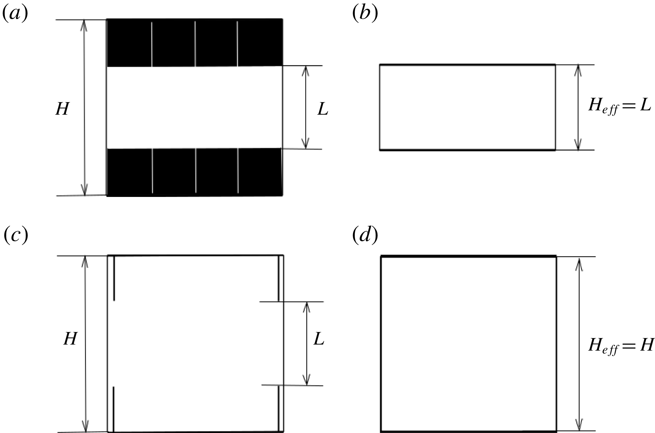
Figure 2. (a,c) Sketches of the convection cells with height $H$
, distance between top and bottom ring-shaped obstacles
$H$
, distance between top and bottom ring-shaped obstacles $L=H-2h$
and height of obstacles
$L=H-2h$
and height of obstacles $h$
, for (a) an infinitesimal gap between the neighbouring obstacles at each plate and (c) an infinitesimal width of each obstacle. (b,d) The reference convection cells with smooth plates, which correspond to the convection cells with obstacles from (a,c), respectively. The effective height
$h$
, for (a) an infinitesimal gap between the neighbouring obstacles at each plate and (c) an infinitesimal width of each obstacle. (b,d) The reference convection cells with smooth plates, which correspond to the convection cells with obstacles from (a,c), respectively. The effective height $H_{eff}$
, which is based on the fluid volume and the area of the central horizontal cross-section of the convection cell, is (a,b)
$H_{eff}$
, which is based on the fluid volume and the area of the central horizontal cross-section of the convection cell, is (a,b) $H_{eff}=L$
and (c,d)
$H_{eff}=L$
and (c,d) $H_{eff}=H$
.
$H_{eff}=H$
.
The Reynolds number $Re$
is determined by the velocity
$Re$
is determined by the velocity $U$
of the turbulent wind in the convection cell, or LSC, which are defined as follows:
$U$
of the turbulent wind in the convection cell, or LSC, which are defined as follows:
 $$\begin{eqnarray}Re=\frac{HU}{\unicode[STIX]{x1D708}},\quad U=\max _{z,z\in (h,H-h)}\sqrt{\langle u_{r}^{2}+u_{\unicode[STIX]{x1D719}}^{2}+u_{z}^{2}\rangle _{z}}.\end{eqnarray}$$
The Nusselt number $Nu$
, Reynolds number
$Nu$
, Reynolds number $Re$
and heat flows from the different parts of the heated plate
$Re$
and heat flows from the different parts of the heated plate $Q_{i}$
,
$Q_{i}$
, $i=1,2,3$
, obtained in the DNS, are summarised in table 1. There one can find also the corresponding effective height
$i=1,2,3$
, obtained in the DNS, are summarised in table 1. There one can find also the corresponding effective height $H_{eff}$
of each considered convection cell and the effective Rayleigh number
$H_{eff}$
of each considered convection cell and the effective Rayleigh number $Ra_{eff}$
, Nusselt number
$Ra_{eff}$
, Nusselt number $Nu_{eff}$
and Reynolds number
$Nu_{eff}$
and Reynolds number $Re_{eff}$
, which are based on
$Re_{eff}$
, which are based on $H_{eff}$
. That is,
$H_{eff}$
. That is,
 $$\begin{eqnarray}Ra_{eff}\equiv (H_{eff}/H)^{3}Ra,\quad Nu_{eff}\equiv (H_{eff}/H)Nu,\quad Re_{eff}\equiv (H_{eff}/H)Re.\end{eqnarray}$$
The effective height $H_{eff}$
is determined by the fluid volume, i.e. by the volume of the cylinder minus the volume of all obstacles, divided by the area of the central horizontal cross-section of the cell, i.e.
$H_{eff}$
is determined by the fluid volume, i.e. by the volume of the cylinder minus the volume of all obstacles, divided by the area of the central horizontal cross-section of the cell, i.e. $A_{s}$
.
$A_{s}$
.
In the rest of the paper the obtained results are presented exclusively for the effective quantities $Ra_{eff}$
,
$Ra_{eff}$
, $Nu_{eff}$
and
$Nu_{eff}$
and $Re_{eff}$
, which are related to the effective height of the convection cell
$Re_{eff}$
, which are related to the effective height of the convection cell $H_{eff}$
, and not for
$H_{eff}$
, and not for $Ra$
,
$Ra$
, $Nu$
and
$Nu$
and $Re$
, which are related to the cylinder height
$Re$
, which are related to the cylinder height $H$
. The reason is that in the case of tall obstacles, the usage of
$H$
. The reason is that in the case of tall obstacles, the usage of $H$
, in contrast to
$H$
, in contrast to $H_{eff}$
, can lead to non-physical results. This is illustrated by figure 2 and explained below.
$H_{eff}$
, can lead to non-physical results. This is illustrated by figure 2 and explained below.
When the obstacles are very wide, so that the gaps between them in the horizontal direction are negligible, the obstacles build a thick plate, and in this case the actual height $h$
of the obstacles no longer matters (see figure 2
a,b). Thus, the reference height in such convection cells should be the distance
$h$
of the obstacles no longer matters (see figure 2
a,b). Thus, the reference height in such convection cells should be the distance $L$
between the top and bottom ring-shaped obstacles,
$L$
between the top and bottom ring-shaped obstacles, $L=H-2h$
. The usage of the reference height
$L=H-2h$
. The usage of the reference height $H$
instead of
$H$
instead of $L$
would lead, in particular, to a value of the Nusselt number that overestimates the actual Nusselt number by a factor of
$L$
would lead, in particular, to a value of the Nusselt number that overestimates the actual Nusselt number by a factor of $H/L$
and to a Rayleigh number overestimated by a factor of
$H/L$
and to a Rayleigh number overestimated by a factor of $(H/L)^{3}$
. In contrast to that, in another limiting case of infinitesimally thin obstacles (see figure 2
c,d), the usage of
$(H/L)^{3}$
. In contrast to that, in another limiting case of infinitesimally thin obstacles (see figure 2
c,d), the usage of $L$
as the reference height of the convection cell would lead to an underestimation of the Nusselt number by a factor of
$L$
as the reference height of the convection cell would lead to an underestimation of the Nusselt number by a factor of $H/L$
and of the Rayleigh number by a factor of
$H/L$
and of the Rayleigh number by a factor of $(H/L)^{3}$
.
$(H/L)^{3}$
.
The usage of the effective height $H_{eff}$
, which is determined by the fluid volume and
$H_{eff}$
, which is determined by the fluid volume and $A_{s}$
, leads to correct reference heights in both limiting cases, which are
$A_{s}$
, leads to correct reference heights in both limiting cases, which are $H_{eff}=L$
in the case of infinitesimal gaps between the neighbouring obstacles (figure 2
a) and
$H_{eff}=L$
in the case of infinitesimal gaps between the neighbouring obstacles (figure 2
a) and $H_{eff}=H$
in the case of an infinitesimal width of the obstacles (figure 2
c). Obviously, when the height of the obstacles, or the plate roughness, is small,
$H_{eff}=H$
in the case of an infinitesimal width of the obstacles (figure 2
c). Obviously, when the height of the obstacles, or the plate roughness, is small, $h\ll H$
, the usage of
$h\ll H$
, the usage of $H_{eff}$
instead of
$H_{eff}$
instead of $H$
is not that influential, but in the case of high and wide obstacles, the usage of the correct effective convection cell height becomes crucial.
$H$
is not that influential, but in the case of high and wide obstacles, the usage of the correct effective convection cell height becomes crucial.
4 Results
Direct numerical simulations of thermal convection in a cylinder of aspect ratio 1, with rough heated and cooled plates or with the ring-shaped obstacles that are attached at the plates, as described in the previous section, have been conducted for 135 different configurations of the ring-shaped obstacles and different numbers of the obstacles, for $Pr=1$
and
$Pr=1$
and $Ra$
from
$Ra$
from $10^{6}$
to
$10^{6}$
to $10^{8}$
. In figure 3 some flows are visualised with three-dimensional isosurfaces of the temperature for
$10^{8}$
. In figure 3 some flows are visualised with three-dimensional isosurfaces of the temperature for $Ra=10^{8}$
, obstacle height
$Ra=10^{8}$
, obstacle height $h/H=0.06$
and different numbers of ring-shaped obstacles.
$h/H=0.06$
and different numbers of ring-shaped obstacles.

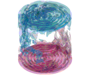
Figure 3. Isosurfaces of the instantaneous temperature distributions, for $Ra=10^{8}$
, height of ring-shaped obstacles
$Ra=10^{8}$
, height of ring-shaped obstacles $h/H=0.06$
and number of rings (a)
$h/H=0.06$
and number of rings (a) $n=2$
, (b)
$n=2$
, (b) $n=4$
and (c)
$n=4$
and (c) $n=8$
. The colour scale ranges from blue (cold fluid) to white (the fluid temperature equals the arithmetic mean of the top and bottom temperatures) to pink (warm fluid).
$n=8$
. The colour scale ranges from blue (cold fluid) to white (the fluid temperature equals the arithmetic mean of the top and bottom temperatures) to pink (warm fluid).
Most of the simulations are conducted for the case of $Ra=10^{7}$
, to study the effects of the gap width, of the obstacle height and of the number of the obstacles. Quantitative information on the studied convective flows is presented in figures 6, 7, 9–11, 13 and 14. The effective Reynolds numbers and Nusselt numbers, obtained in the DNS, are presented in table 1. To visualise different DNS results, the symbols according to table 2 are used in the figures throughout the paper.
$Ra=10^{7}$
, to study the effects of the gap width, of the obstacle height and of the number of the obstacles. Quantitative information on the studied convective flows is presented in figures 6, 7, 9–11, 13 and 14. The effective Reynolds numbers and Nusselt numbers, obtained in the DNS, are presented in table 1. To visualise different DNS results, the symbols according to table 2 are used in the figures throughout the paper.

4.1 The influence of the width of the gaps between the obstacles
From previous studies of the effect of plate roughness in thermal convection (see, e.g. Roche et al.
Reference Roche, Castaing, Chabaud and Herbal2001), it is known that the influence of the roughness on the mean heat transport is negligible when the roughness height is smaller than or comparable to the thickness $\unicode[STIX]{x1D6FF}_{\unicode[STIX]{x1D703}}$
of the thermal boundary layer in the smooth-plate case. In the smooth-plate case, the thickness of the thermal boundary layer is
$\unicode[STIX]{x1D6FF}_{\unicode[STIX]{x1D703}}$
of the thermal boundary layer in the smooth-plate case. In the smooth-plate case, the thickness of the thermal boundary layer is
 $$\begin{eqnarray}\unicode[STIX]{x1D6FF}_{\unicode[STIX]{x1D703}}=H/(2Nu_{s}),\end{eqnarray}$$
where $Nu_{s}$
is the Nusselt number in the smooth-plate case. When the obstacle height
$Nu_{s}$
is the Nusselt number in the smooth-plate case. When the obstacle height $h$
is larger than
$h$
is larger than $\unicode[STIX]{x1D6FF}_{\unicode[STIX]{x1D703}}$
, the mean heat transport, i.e. the Nusselt number, can be different from that in the smooth-plate case. Usually, the presence of obstacles at the heated and cooled plates, which have the same temperature as the corresponding plate, leads to an increase of the Nusselt number compared to the smooth-plate case. The Nusselt numbers for the studied smooth-plate cases,
$\unicode[STIX]{x1D6FF}_{\unicode[STIX]{x1D703}}$
, the mean heat transport, i.e. the Nusselt number, can be different from that in the smooth-plate case. Usually, the presence of obstacles at the heated and cooled plates, which have the same temperature as the corresponding plate, leads to an increase of the Nusselt number compared to the smooth-plate case. The Nusselt numbers for the studied smooth-plate cases, $Nu_{s}$
, can be found in table 1 for
$Nu_{s}$
, can be found in table 1 for $n\,=\,0$
. For the smooth cases,
$n\,=\,0$
. For the smooth cases, $Nu_{s}=Nu=Nu_{eff}$
, and from these values the corresponding thicknesses of the thermal boundary layers can be calculated, according to relation (4.1).
$Nu_{s}=Nu=Nu_{eff}$
, and from these values the corresponding thicknesses of the thermal boundary layers can be calculated, according to relation (4.1).
To investigate the influence of the width of the gap between the obstacles, for a fixed number $n=2$
of the ring-shaped obstacles, we consider a set of different obstacle heights, more precisely,
$n=2$
of the ring-shaped obstacles, we consider a set of different obstacle heights, more precisely, $h/H=0.015$
,
$h/H=0.015$
, $0.03$
,
$0.03$
, $0.06$
,
$0.06$
, $0.12$
and
$0.12$
and $0.25$
, and for each of the chosen
$0.25$
, and for each of the chosen $h$
, the DNS have been conducted for different widths of the gap
$h$
, the DNS have been conducted for different widths of the gap $a$
between the obstacles. The considered cases are
$a$
between the obstacles. The considered cases are $a/H=0.015$
, 0.03, 0.06, 0.104, 0.12, 0.152, 0.176 and 0.188.
$a/H=0.015$
, 0.03, 0.06, 0.104, 0.12, 0.152, 0.176 and 0.188.

Figure 4. Snapshots of the flow fields (temperature and streamlines) in the central vertical cross-sections, for $Ra=10^{7}$
, number of ring-shaped obstacles
$Ra=10^{7}$
, number of ring-shaped obstacles $n=2$
, obstacle height
$n=2$
, obstacle height $h/H=0.015$
and gap between obstacles (a)
$h/H=0.015$
and gap between obstacles (a) $a/H=0.015$
, (b)
$a/H=0.015$
, (b) $a/H=0.104$
and (c)
$a/H=0.104$
and (c) $a/H=0.188$
. The temperature colour scale ranges from blue (cold fluid) to white (the fluid temperature is
$a/H=0.188$
. The temperature colour scale ranges from blue (cold fluid) to white (the fluid temperature is $T_{m}\equiv (T_{+}+T_{-})/2$
, the arithmetic mean of the top and bottom temperatures) to pink (warm fluid).
$T_{m}\equiv (T_{+}+T_{-})/2$
, the arithmetic mean of the top and bottom temperatures) to pink (warm fluid).
In the case of $Ra=10^{7}$
, for
$Ra=10^{7}$
, for $h/H=0.015$
(see figure 4), the height of the obstacles is smaller than the thickness of the thermal boundary layer in the smooth-plate case, and therefore the width of the gap between the obstacles does not have much influence, since for any
$h/H=0.015$
(see figure 4), the height of the obstacles is smaller than the thickness of the thermal boundary layer in the smooth-plate case, and therefore the width of the gap between the obstacles does not have much influence, since for any $a$
, most of the time, the obstacles are covered by the thermal boundary layer and do not influence the heat transport.
$a$
, most of the time, the obstacles are covered by the thermal boundary layer and do not influence the heat transport.

Figure 5. Snapshots of the flow fields in the central vertical cross-sections, for $Ra=10^{7}$
, number of ring-shaped obstacles
$Ra=10^{7}$
, number of ring-shaped obstacles $n=2$
, obstacle height
$n=2$
, obstacle height $h/H=0.25$
and gap between obstacles (a)
$h/H=0.25$
and gap between obstacles (a) $a/H=0.015$
, (b)
$a/H=0.015$
, (b) $a/H=0.104$
and (c)
$a/H=0.104$
and (c) $a/H=0.188$
. The colour scale is as in figure 4.
$a/H=0.188$
. The colour scale is as in figure 4.
A completely different situation is observed for tall obstacles, $h/H=0.25$
, and
$h/H=0.25$
, and $Ra=10^{7}$
. Here, for the same gaps between the obstacles as in figure 4, one obtains a strong dependence of the flow structure on the gap width
$Ra=10^{7}$
. Here, for the same gaps between the obstacles as in figure 4, one obtains a strong dependence of the flow structure on the gap width $a$
. This is illustrated in figure 5. When the gap is very thin (
$a$
. This is illustrated in figure 5. When the gap is very thin ( $a/H=0.015$
), the fluid stagnates between the heated as well as between the cooled obstacles (figure 5
a), and thus the global flow structure is expected to be similar to that in RBC in a cylindrical container of aspect ratio
$a/H=0.015$
), the fluid stagnates between the heated as well as between the cooled obstacles (figure 5
a), and thus the global flow structure is expected to be similar to that in RBC in a cylindrical container of aspect ratio $2R/(H-2h)=2$
, with smooth plates, and with the Rayleigh number reduced by a factor
$2R/(H-2h)=2$
, with smooth plates, and with the Rayleigh number reduced by a factor $((H-2h)/H)^{3}=1/8$
.
$((H-2h)/H)^{3}=1/8$
.
With increasing height of the obstacles, as soon as $h$
becomes larger than
$h$
becomes larger than $\unicode[STIX]{x1D6FF}_{\unicode[STIX]{x1D703}}$
, the obstacles start to contribute to the heat transport in the system. For a sufficiently large gap between the obstacles,
$\unicode[STIX]{x1D6FF}_{\unicode[STIX]{x1D703}}$
, the obstacles start to contribute to the heat transport in the system. For a sufficiently large gap between the obstacles, $a/H=0.104$
, from time to time, the fluid is completely washed out from the gaps between the obstacles, and thus the heated and cooled obstacles contribute to the heat transport in the system (see figure 5
b). Here one can expect a significant increase of the Nusselt number, compared to the smooth-plate case.
$a/H=0.104$
, from time to time, the fluid is completely washed out from the gaps between the obstacles, and thus the heated and cooled obstacles contribute to the heat transport in the system (see figure 5
b). Here one can expect a significant increase of the Nusselt number, compared to the smooth-plate case.
After a certain sufficiently large value of $a$
, when the obstacles are already strongly washed from all sides that are open to the fluid, a further increase of
$a$
, when the obstacles are already strongly washed from all sides that are open to the fluid, a further increase of $a$
might not lead to an increase of the Nusselt number, since no additional heated or cooled surfaces get involved in the heat transport process with the increase of the gap between the obstacles (see figure 5
c). In this respect, for tall roughness elements, we might expect the existence of an optimal geometrical configuration of the roughness elements that provide the maximal heat transport in the system, similar to the standard confined RBC with adiabatic sidewalls (Chong et al.
Reference Chong, Wagner, Kaczorowski, Shishkina and Xia2018).
$a$
might not lead to an increase of the Nusselt number, since no additional heated or cooled surfaces get involved in the heat transport process with the increase of the gap between the obstacles (see figure 5
c). In this respect, for tall roughness elements, we might expect the existence of an optimal geometrical configuration of the roughness elements that provide the maximal heat transport in the system, similar to the standard confined RBC with adiabatic sidewalls (Chong et al.
Reference Chong, Wagner, Kaczorowski, Shishkina and Xia2018).

Figure 6. Dependences of the normalised effective (a,c) Nusselt number $Nu_{eff}$
and (b,d) Reynolds number
$Nu_{eff}$
and (b,d) Reynolds number $Re_{eff}$
on the gap
$Re_{eff}$
on the gap $a$
between one or two ring-shaped obstacles, for
$a$
between one or two ring-shaped obstacles, for $Ra=10^{6}$
and obstacle height
$Ra=10^{6}$
and obstacle height $h/H=0.12$
, for
$h/H=0.12$
, for $Ra=10^{7}$
and
$Ra=10^{7}$
and $h/H=0.015$
, 0.03, 0.06, 0.12 and 0.25 and for
$h/H=0.015$
, 0.03, 0.06, 0.12 and 0.25 and for $Ra=10^{8}$
and
$Ra=10^{8}$
and $h/H=0.06$
and 0.12 (see symbol meanings in table 2). Here
$h/H=0.06$
and 0.12 (see symbol meanings in table 2). Here $Nu_{eff}$
and
$Nu_{eff}$
and $Re_{eff}$
are normalised with respect to the Nusselt number
$Re_{eff}$
are normalised with respect to the Nusselt number $Nu_{s}$ $(a)$
and Reynolds number
$(a)$
and Reynolds number $Re_{s}$ $(b)$
that correspond to
$(b)$
that correspond to $Ra=Ra_{eff}$
in the smooth-plate case (see equations (4.2) and (4.3)). In (c,d) the data are plotted versus the gap
$Ra=Ra_{eff}$
in the smooth-plate case (see equations (4.2) and (4.3)). In (c,d) the data are plotted versus the gap $a$
, normalised with the thickness of the thermal boundary layer in the smooth case for
$a$
, normalised with the thickness of the thermal boundary layer in the smooth case for $Ra=Ra_{eff}$
, i.e. with
$Ra=Ra_{eff}$
, i.e. with $\unicode[STIX]{x1D6FF}_{\unicode[STIX]{x1D703}}=H_{eff}/(2Nu_{s})$
.
$\unicode[STIX]{x1D6FF}_{\unicode[STIX]{x1D703}}=H_{eff}/(2Nu_{s})$
.
The dependences of the effective Nusselt number $Nu_{eff}$
, normalised with
$Nu_{eff}$
, normalised with $Nu_{s}$
, and the effective Reynolds number
$Nu_{s}$
, and the effective Reynolds number $Re_{eff}$
, normalised with
$Re_{eff}$
, normalised with $Re_{s}$
, as functions of the gap width between the obstacles,
$Re_{s}$
, as functions of the gap width between the obstacles, $a$
, are presented, respectively, in figures 6(a) and 6(b), for
$a$
, are presented, respectively, in figures 6(a) and 6(b), for $Ra=10^{6}$
,
$Ra=10^{6}$
, $10^{7}$
and
$10^{7}$
and $10^{8}$
, number of ring-shaped obstacles
$10^{8}$
, number of ring-shaped obstacles $n=1$
or
$n=1$
or $n=2$
and different combinations of the obstacle heights
$n=2$
and different combinations of the obstacle heights $h$
. Here
$h$
. Here $Nu_{s}$
and
$Nu_{s}$
and $Re_{s}$
are, respectively, the Nusselt number and Reynolds number in classical RBC with smooth plates, for
$Re_{s}$
are, respectively, the Nusselt number and Reynolds number in classical RBC with smooth plates, for $Ra=Ra_{eff}$
. For each particular value of
$Ra=Ra_{eff}$
. For each particular value of $Ra=Ra_{eff}$
, the values of
$Ra=Ra_{eff}$
, the values of $Nu_{s}$
and
$Nu_{s}$
and $Re_{s}$
are calculated according to the formulas
$Re_{s}$
are calculated according to the formulas
 $$\begin{eqnarray}\displaystyle & \displaystyle Nu_{s}=0.166Ra^{0.286}, & \displaystyle\end{eqnarray}$$
 $$\begin{eqnarray}\displaystyle & \displaystyle Re_{s}=0.191Ra^{0.492}, & \displaystyle\end{eqnarray}$$
which are obtained from the power-law fitting of the DNS data for classical RBC with smooth plates, for $Ra$
from
$Ra$
from $10^{6}$
to
$10^{6}$
to $10^{8}$
.
$10^{8}$
.
One can see that the normalised effective Nusselt number is generally larger for larger $a$
(see figure 6
a). The data points for larger obstacle heights show larger effective Nusselt numbers than the data points for lower
$a$
(see figure 6
a). The data points for larger obstacle heights show larger effective Nusselt numbers than the data points for lower $h$
. This means that the presence of tall obstacles can potentially lead to stronger heat transport enhancement, if the gap between the obstacles is sufficiently large. As is expected from the analysis of figure 4, an increase of the gap does not lead to an increase of the Nusselt number if the obstacle height is small, and this is supported by the example of
$h$
. This means that the presence of tall obstacles can potentially lead to stronger heat transport enhancement, if the gap between the obstacles is sufficiently large. As is expected from the analysis of figure 4, an increase of the gap does not lead to an increase of the Nusselt number if the obstacle height is small, and this is supported by the example of $h/H=0.015$
in figure 6(a) (downward triangles). Opposite to this situation, for tall obstacles, the gap width becomes important, and with growing
$h/H=0.015$
in figure 6(a) (downward triangles). Opposite to this situation, for tall obstacles, the gap width becomes important, and with growing $a$
, the heat transport is significantly increased compared to the smooth-plate case, as can be seen by the example of
$a$
, the heat transport is significantly increased compared to the smooth-plate case, as can be seen by the example of $h/H=0.25$
(upward triangles in figure 6
a). A fast growth of the normalised effective Nusselt number with growing
$h/H=0.25$
(upward triangles in figure 6
a). A fast growth of the normalised effective Nusselt number with growing $a$
for the case
$a$
for the case $h/H=0.25$
is observed in the interval
$h/H=0.25$
is observed in the interval $a/H\in [0;0.104]$
. When the gap width is about
$a/H\in [0;0.104]$
. When the gap width is about $a/H=0.104$
, the cavities between the neighbouring obstacles of the same temperature are already fully and regularly washed out (see also figure 5
a), and further increase of the gap width does not lead to an increase of the Nusselt number.
$a/H=0.104$
, the cavities between the neighbouring obstacles of the same temperature are already fully and regularly washed out (see also figure 5
a), and further increase of the gap width does not lead to an increase of the Nusselt number.
In figure 6(c) the same data (as in figure 6
a) are plotted versus the gap width $a$
, normalised with the corresponding thickness of the thermal boundary layer (
$a$
, normalised with the corresponding thickness of the thermal boundary layer ( $\unicode[STIX]{x1D6FF}_{\unicode[STIX]{x1D703}}$
). One sees that for tall roughness elements, the Nusselt number increases fast for
$\unicode[STIX]{x1D6FF}_{\unicode[STIX]{x1D703}}$
). One sees that for tall roughness elements, the Nusselt number increases fast for $a$
up to approximately
$a$
up to approximately $4\unicode[STIX]{x1D6FF}_{\unicode[STIX]{x1D703}}$
. After that, a further increase of the gap width does not much influence the heat transport.
$4\unicode[STIX]{x1D6FF}_{\unicode[STIX]{x1D703}}$
. After that, a further increase of the gap width does not much influence the heat transport.
The normalised effective Reynolds numbers, presented in figure 6(b), demonstrate a non-monotonic behaviour with the gap width $a$
. First, as the gap is small, this quantity grows with growing
$a$
. First, as the gap is small, this quantity grows with growing $a$
, due to additional heated/cooled surfaces, and the LSC remains unconstrained by the obstacles (see also figure 5
a). As soon as the cavities between the obstacles are involved in the convective process, the LSC becomes less pronounced, its structure becomes more complicated (see figure 5
c) and its strength starts to reduce, which is reflected in a slight reduction of of the normalised Reynolds number for large gaps between the obstacles. Similar (to a certain extent) observations with respect to the normalised Nusselt numbers and Reynolds numbers were reported in previous numerical studies, e.g. in Toppaladoddi, Succi & Wettlaufer (Reference Toppaladoddi, Succi and Wettlaufer2015) and Wagner & Shishkina (Reference Wagner and Shishkina2015).
$a$
, due to additional heated/cooled surfaces, and the LSC remains unconstrained by the obstacles (see also figure 5
a). As soon as the cavities between the obstacles are involved in the convective process, the LSC becomes less pronounced, its structure becomes more complicated (see figure 5
c) and its strength starts to reduce, which is reflected in a slight reduction of of the normalised Reynolds number for large gaps between the obstacles. Similar (to a certain extent) observations with respect to the normalised Nusselt numbers and Reynolds numbers were reported in previous numerical studies, e.g. in Toppaladoddi, Succi & Wettlaufer (Reference Toppaladoddi, Succi and Wettlaufer2015) and Wagner & Shishkina (Reference Wagner and Shishkina2015).

Figure 7. Dependences of the normalised effective Nusselt number $Nu_{eff}$
on the effective (a) Rayleigh number
$Nu_{eff}$
on the effective (a) Rayleigh number $Ra_{eff}$
and (b) height
$Ra_{eff}$
and (b) height $H_{eff}$
, for the cases as in figure 6. Symbols are according to table 2. The data are normalised with respect to the Nusselt number
$H_{eff}$
, for the cases as in figure 6. Symbols are according to table 2. The data are normalised with respect to the Nusselt number $Nu_{s}$
that corresponds to
$Nu_{s}$
that corresponds to $Ra=Ra_{eff}$
in the smooth-plate case (see (4.2)).
$Ra=Ra_{eff}$
in the smooth-plate case (see (4.2)).
In figure 7, the normalised effective Nusselt numbers are plotted against the effective Rayleigh numbers $Ra_{eff}$
(figure 7
a) and the effective heights
$Ra_{eff}$
(figure 7
a) and the effective heights $H_{eff}$
(figure 7
b). In figure 7(a), for any fixed
$H_{eff}$
(figure 7
b). In figure 7(a), for any fixed $Ra$
, the values of
$Ra$
, the values of $Ra_{eff}$
are larger for larger volume of the fluid, which, in the case of a fixed obstacle height, is equivalent to larger width of the gaps between the obstacles. One can see in figure 7(a) that the normalised effective Nusselt number in the case of the rough plates is not always larger than that in the case of the smooth plates; sometimes, e.g. for small gaps between the obstacles, it can be smaller than that in the smooth-plate case. This finding is in good agreement with the earlier studies by Shishkina & Wagner (Reference Shishkina and Wagner2011) and Zhang et al. (Reference Zhang, Sun, Bao and Zhou2018). The Nusselt number reduction happens only in a few cases and is possible only for small
$Ra_{eff}$
are larger for larger volume of the fluid, which, in the case of a fixed obstacle height, is equivalent to larger width of the gaps between the obstacles. One can see in figure 7(a) that the normalised effective Nusselt number in the case of the rough plates is not always larger than that in the case of the smooth plates; sometimes, e.g. for small gaps between the obstacles, it can be smaller than that in the smooth-plate case. This finding is in good agreement with the earlier studies by Shishkina & Wagner (Reference Shishkina and Wagner2011) and Zhang et al. (Reference Zhang, Sun, Bao and Zhou2018). The Nusselt number reduction happens only in a few cases and is possible only for small $Ra$
. In particular, one can see this for the
$Ra$
. In particular, one can see this for the $Ra=10^{6}$
data, which in figure 7(a) are presented by the lower-filled symbols. For large
$Ra=10^{6}$
data, which in figure 7(a) are presented by the lower-filled symbols. For large $Ra$
, the presence of the obstacles, or plate roughness, always leads to an increase of the mean heat transport (see the upper-filled data points in figure 7
a for
$Ra$
, the presence of the obstacles, or plate roughness, always leads to an increase of the mean heat transport (see the upper-filled data points in figure 7
a for $Ra=10^{8}$
).
$Ra=10^{8}$
).
4.2 The influence of the obstacle height
To investigate the influence of the obstacle height $h$
, we consider a set of different widths
$h$
, we consider a set of different widths $a$
between the isothermal obstacles, more precisely
$a$
between the isothermal obstacles, more precisely $a/H=0.015$
, 0.03, 0.06, 0.104, 0.12, 0.152, 0.176 and 0.188, for different numbers of the ring-shaped obstacles. For each of the chosen
$a/H=0.015$
, 0.03, 0.06, 0.104, 0.12, 0.152, 0.176 and 0.188, for different numbers of the ring-shaped obstacles. For each of the chosen $a$
, the DNS data are analysed with respect to their dependence on the obstacle height
$a$
, the DNS data are analysed with respect to their dependence on the obstacle height $h$
. The considered heights are
$h$
. The considered heights are $h/H=0.015$
, 0.03, 0.06, 0.12, 0.25, 0.4 and 0.49.
$h/H=0.015$
, 0.03, 0.06, 0.12, 0.25, 0.4 and 0.49.

Figure 8. Snapshots of the flow fields in the central vertical cross-sections, for $Ra=10^{7}$
, number of ring-shaped obstacles
$Ra=10^{7}$
, number of ring-shaped obstacles $n=4$
, gap between obstacles
$n=4$
, gap between obstacles $a/H=0.10$
and obstacle height (a)
$a/H=0.10$
and obstacle height (a) $h/H=0.015$
, (b)
$h/H=0.015$
, (b) $h/H=0.25$
and (c)
$h/H=0.25$
and (c) $h/H=0.4$
. The colour scale is as in figure 4.
$h/H=0.4$
. The colour scale is as in figure 4.
In figure 8, for three different obstacle heights, the instantaneous temperature distributions and streamlines are presented for $Ra=10^{7}$
, number of ring-shaped obstacles
$Ra=10^{7}$
, number of ring-shaped obstacles $n=4$
and width of gaps between them
$n=4$
and width of gaps between them $a/H=0.10$
. In the case of short obstacles,
$a/H=0.10$
. In the case of short obstacles, $h/H=0.015$
, the roughness is embedded into the thermal boundary layer, the LSC is not affected and, therefore, one can expect an effective Nusselt number similar to that in the case of the smooth plates (see figure 8
a). For a significantly larger obstacle height,
$h/H=0.015$
, the roughness is embedded into the thermal boundary layer, the LSC is not affected and, therefore, one can expect an effective Nusselt number similar to that in the case of the smooth plates (see figure 8
a). For a significantly larger obstacle height, $h/H=0.25$
(figure 8
b), the obstacles contribute to the global heat transport, as the flow is present also between the isothermal obstacles in this case.
$h/H=0.25$
(figure 8
b), the obstacles contribute to the global heat transport, as the flow is present also between the isothermal obstacles in this case.
With a further increase of the obstacle height, $h/H=0.4$
(figure 8
c), the LSC is deformed in such a way that it often takes the form of a set of rolls in the gaps between the neighbouring obstacles of the same temperature, and these rolls extend from the very bottom to the very top of the convection cell. Note that such a change of the global flow structure can also lead to an increase of the Nusselt number. As was shown in a study of the effect of the RBC cell confinement on the heat transport (Chong et al.
Reference Chong, Wagner, Kaczorowski, Shishkina and Xia2018), for
$h/H=0.4$
(figure 8
c), the LSC is deformed in such a way that it often takes the form of a set of rolls in the gaps between the neighbouring obstacles of the same temperature, and these rolls extend from the very bottom to the very top of the convection cell. Note that such a change of the global flow structure can also lead to an increase of the Nusselt number. As was shown in a study of the effect of the RBC cell confinement on the heat transport (Chong et al.
Reference Chong, Wagner, Kaczorowski, Shishkina and Xia2018), for $Pr\geqslant 1$
, there exists an optimal width-to-height aspect ratio of the RBC cell that provides a maximal heat transport and this optimal aspect ratio is about 0.1 for
$Pr\geqslant 1$
, there exists an optimal width-to-height aspect ratio of the RBC cell that provides a maximal heat transport and this optimal aspect ratio is about 0.1 for $Pr=1$
and decreases with growing
$Pr=1$
and decreases with growing $Ra$
and
$Ra$
and $Pr$
. Therefore the tendency of the global flow to take the form of a set of separate rolls between the neighbouring obstacles can also increase the total heat transport, compared to the singe-roll LSC that takes place in the classical RBC with smooth plates. In the case of extremely tall obstacles and sufficiently large gaps between them, both horizontal and vertical heated/cooled surfaces can contribute to the increase of the heat transport in the system, where the increasing contribution from the vertical walls of the roughness elements can grow almost linearly with their height.
$Pr$
. Therefore the tendency of the global flow to take the form of a set of separate rolls between the neighbouring obstacles can also increase the total heat transport, compared to the singe-roll LSC that takes place in the classical RBC with smooth plates. In the case of extremely tall obstacles and sufficiently large gaps between them, both horizontal and vertical heated/cooled surfaces can contribute to the increase of the heat transport in the system, where the increasing contribution from the vertical walls of the roughness elements can grow almost linearly with their height.

Figure 9. Dependences of the effective (a,c) Nusselt number $Nu_{eff}$
and (b,d) Reynolds number
$Nu_{eff}$
and (b,d) Reynolds number $Re_{eff}$
on the height
$Re_{eff}$
on the height $h$
of the ring-shaped obstacles, for
$h$
of the ring-shaped obstacles, for $Ra=10^{7}$
and
$Ra=10^{7}$
and $n=1$
ring with the gap
$n=1$
ring with the gap $a/H=0.015$
, for
$a/H=0.015$
, for $Ra=10^{7}$
and
$Ra=10^{7}$
and $n=2$
ring-shaped obstacles and the gap varying from
$n=2$
ring-shaped obstacles and the gap varying from $a/H=0.015$
to 0.188 and for
$a/H=0.015$
to 0.188 and for $Ra=10^{7}$
and
$Ra=10^{7}$
and $n=4$
ring-shaped obstacles and the gap between them
$n=4$
ring-shaped obstacles and the gap between them $a/H=0.10$
(see symbol meanings in table 2). The values of
$a/H=0.10$
(see symbol meanings in table 2). The values of $Nu_{eff}$
and
$Nu_{eff}$
and $Re_{eff}$
are normalised with respect to the Nusselt number
$Re_{eff}$
are normalised with respect to the Nusselt number $Nu_{s}$ $(a)$
and Reynolds number
$(a)$
and Reynolds number $Re_{s}$ $(b)$
that correspond to
$(b)$
that correspond to $Ra=Ra_{eff}$
in the smooth-plate case (see (4.2) and (4.3)). In (c,d) the data are plotted versus the roughness height
$Ra=Ra_{eff}$
in the smooth-plate case (see (4.2) and (4.3)). In (c,d) the data are plotted versus the roughness height $h$
, normalised with the thickness of the thermal boundary layer in the smooth case for
$h$
, normalised with the thickness of the thermal boundary layer in the smooth case for $Ra=Ra_{eff}$
, i.e. with
$Ra=Ra_{eff}$
, i.e. with $\unicode[STIX]{x1D6FF}_{\unicode[STIX]{x1D703}}=H_{eff}/(2Nu_{s})$
.
$\unicode[STIX]{x1D6FF}_{\unicode[STIX]{x1D703}}=H_{eff}/(2Nu_{s})$
.
The dependences of the normalised effective Nusselt number $Nu_{eff}$
and Reynolds number
$Nu_{eff}$
and Reynolds number $Re_{eff}$
as functions of the obstacle height
$Re_{eff}$
as functions of the obstacle height $h$
are presented, respectively, in figures 9(a) and 9(b), for
$h$
are presented, respectively, in figures 9(a) and 9(b), for $Ra=10^{7}$
, different numbers of ring-shaped obstacles and various widths
$Ra=10^{7}$
, different numbers of ring-shaped obstacles and various widths $a$
of the gaps between the obstacles. One can see that the value of
$a$
of the gaps between the obstacles. One can see that the value of $Nu_{eff}/Nu_{s}$
generally increases almost linearly with increasing height of the obstacles.
$Nu_{eff}/Nu_{s}$
generally increases almost linearly with increasing height of the obstacles.
When the distance between the neighbouring obstacles is very small, i.e. it is smaller than the double thickness of the thermal boundary layer in the smooth-plate case, as it is for $a/H=0.015$
or
$a/H=0.015$
or $a/H=0.03$
, the height of the obstacles does not matter: for any obstacle height the normalised effective Nusselt number is almost indistinguishable from that in the smooth-plate case. The change of the effective aspect ratio of the container has little influence. For
$a/H=0.03$
, the height of the obstacles does not matter: for any obstacle height the normalised effective Nusselt number is almost indistinguishable from that in the smooth-plate case. The change of the effective aspect ratio of the container has little influence. For $a/H=0.06$
(side-filled diamonds in figure 9
a), the gap between the obstacles is already sufficiently large to allow the flows to skim the hot fluid between the bottom obstacles and the cold fluid between the top obstacles, and therefore an increase of the Nusselt number compared to the smooth-plate case is observed. Very impressive is the collapse of the data in figure 9(a) for
$a/H=0.06$
(side-filled diamonds in figure 9
a), the gap between the obstacles is already sufficiently large to allow the flows to skim the hot fluid between the bottom obstacles and the cold fluid between the top obstacles, and therefore an increase of the Nusselt number compared to the smooth-plate case is observed. Very impressive is the collapse of the data in figure 9(a) for $Ra=10^{7}$
,
$Ra=10^{7}$
, $n=2$
and any of the gap widths
$n=2$
and any of the gap widths $a/H=0.104$
, 0.12, 0.152, 0.176 and 0.188. This again supports the fact that as soon as the cavities between the neighbouring obstacles are washed out, a further increase of the gap between the obstacles does not lead to any change of the effective Nusselt number. The slope of the growth of
$a/H=0.104$
, 0.12, 0.152, 0.176 and 0.188. This again supports the fact that as soon as the cavities between the neighbouring obstacles are washed out, a further increase of the gap between the obstacles does not lead to any change of the effective Nusselt number. The slope of the growth of $Nu_{eff}/Nu_{s}$
with growing
$Nu_{eff}/Nu_{s}$
with growing $h$
is steeper for a larger number of the well-separated obstacles, as one can conclude from a comparison of the data points for
$h$
is steeper for a larger number of the well-separated obstacles, as one can conclude from a comparison of the data points for $Ra=10^{7}$
,
$Ra=10^{7}$
, $n=4$
and
$n=4$
and $a/H=0.10$
with the other results presented for a smaller number of the obstacles (figures 9
a and 9
c).
$a/H=0.10$
with the other results presented for a smaller number of the obstacles (figures 9
a and 9
c).
For small and moderate $h$
, the normalised effective Reynolds number,
$h$
, the normalised effective Reynolds number, $Re_{eff}/Re_{s}$
, grows with the increasing height of the obstacles (see figure 9
b). When the obstacles are extremely tall, as in the case of
$Re_{eff}/Re_{s}$
, grows with the increasing height of the obstacles (see figure 9
b). When the obstacles are extremely tall, as in the case of $h/H=0.4$
, the global flow structure is modified, as discussed above with respect to figure 8(c), the LSC is confined, and this results in a reduction of
$h/H=0.4$
, the global flow structure is modified, as discussed above with respect to figure 8(c), the LSC is confined, and this results in a reduction of $Re_{eff}/Re_{s}$
.
$Re_{eff}/Re_{s}$
.

Figure 10. Dependences of the normalised effective Nusselt number $Nu_{eff}$
on the effective (a) Rayleigh number
$Nu_{eff}$
on the effective (a) Rayleigh number $Ra_{eff}$
and (b) height
$Ra_{eff}$
and (b) height $H_{eff}$
, for the cases as in figure 9. Symbols are according to table 2. The data are normalised with respect to the Nusselt number
$H_{eff}$
, for the cases as in figure 9. Symbols are according to table 2. The data are normalised with respect to the Nusselt number $Nu_{s}$
that corresponds to
$Nu_{s}$
that corresponds to $Ra=Ra_{eff}$
in the smooth-plate case (see (4.2)).
$Ra=Ra_{eff}$
in the smooth-plate case (see (4.2)).
In figure 10, the normalised effective Nusselt numbers are plotted against the effective Rayleigh numbers $Ra_{eff}$
(figure 10
a) and the effective heights
$Ra_{eff}$
(figure 10
a) and the effective heights $H_{eff}$
(figure 10
b). In figure 10(a), for any fixed
$H_{eff}$
(figure 10
b). In figure 10(a), for any fixed $Ra$
, the values of
$Ra$
, the values of $Ra_{eff}$
are larger for larger fluid volume, which, in the case of a fixed distance between the ring-shaped obstacles, is equivalent to shorter obstacles. Thus, for a sufficiently large gap, taller obstacles generally mean larger effective Nusselt numbers (see figure 10
a).
$Ra_{eff}$
are larger for larger fluid volume, which, in the case of a fixed distance between the ring-shaped obstacles, is equivalent to shorter obstacles. Thus, for a sufficiently large gap, taller obstacles generally mean larger effective Nusselt numbers (see figure 10
a).
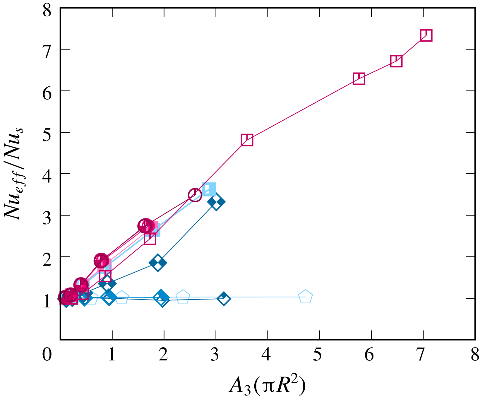
Figure 11. Dependence of the normalised effective Nusselt number $Nu_{eff}$
on the relative additional surface area of the plates due to the presence of the obstacles (i.e. the relative area of the sidewalls of the ring-shaped obstacles), for the cases as in figure 9. Symbols are according to table 2. The data are normalised with respect to the Nusselt number
$Nu_{eff}$
on the relative additional surface area of the plates due to the presence of the obstacles (i.e. the relative area of the sidewalls of the ring-shaped obstacles), for the cases as in figure 9. Symbols are according to table 2. The data are normalised with respect to the Nusselt number $Nu_{s}$
that corresponds to
$Nu_{s}$
that corresponds to $Ra=Ra_{eff}$
in the smooth-plate case (see (4.2)).
$Ra=Ra_{eff}$
in the smooth-plate case (see (4.2)).
In figure 11, the normalised effective Nusselt numbers are plotted against the relative additional area of the plates due to the presence of the obstacles, for the same obstacle configurations as considered in figures 9 and 10. This additional area occurs from the sidewalls of the obstacles and is proportional to the obstacle height. In the case of a fixed gap between the roughness elements, the additional area is proportional to the roughness element height and, therefore, this figure is similar to figure 9(a).
4.3 The influence of the number of the ring-shaped obstacles
In figure 12, snapshots of the flows are presented for $Ra=10^{8}$
and different numbers
$Ra=10^{8}$
and different numbers $n$
of the ring-shaped obstacles, which are separated by sufficiently large gaps of width
$n$
of the ring-shaped obstacles, which are separated by sufficiently large gaps of width $a/H\geqslant 0.10$
. The dependences of the normalised effective Nusselt number
$a/H\geqslant 0.10$
. The dependences of the normalised effective Nusselt number $Nu_{eff}$
and Reynolds number
$Nu_{eff}$
and Reynolds number $Re_{eff}$
on the effective Rayleigh number
$Re_{eff}$
on the effective Rayleigh number $Ra_{eff}$
for some fixed combinations of
$Ra_{eff}$
for some fixed combinations of $a$
,
$a$
, $h$
and
$h$
and $n$
are presented in figure 13. One can see that a larger number of obstacles generally leads to a larger mean heat transport. For relatively thin gaps between the obstacles (i.e. when the ratio between the gap width and the thickness of the thermal boundary layer is relatively small, which for any prescribed value of
$n$
are presented in figure 13. One can see that a larger number of obstacles generally leads to a larger mean heat transport. For relatively thin gaps between the obstacles (i.e. when the ratio between the gap width and the thickness of the thermal boundary layer is relatively small, which for any prescribed value of $a$
corresponds to smaller values of
$a$
corresponds to smaller values of $Ra_{eff}$
in figure 13), the fluid is trapped in the obstacle gaps, but only partly, and therefore in this
$Ra_{eff}$
in figure 13), the fluid is trapped in the obstacle gaps, but only partly, and therefore in this $Ra_{eff}$
region, not only is the mean heat transport increased, but also the scaling exponent in the effective Nusselt number versus the effective Rayleigh number scaling is increased. This is especially well pronounced in the case of
$Ra_{eff}$
region, not only is the mean heat transport increased, but also the scaling exponent in the effective Nusselt number versus the effective Rayleigh number scaling is increased. This is especially well pronounced in the case of $n=4$
rings and
$n=4$
rings and $a/H=0.1$
. When the relative gap width (compared to the thickness of the thermal boundary layer) becomes sufficiently large (large
$a/H=0.1$
. When the relative gap width (compared to the thickness of the thermal boundary layer) becomes sufficiently large (large $Ra_{eff}$
in figure 13
a), the scaling exponent decreases back, slowly approaching that in the smooth-plate case. The scaling of the effective Reynolds number with the effective Rayleigh number is weakly influenced by the number of obstacles (see figure 13
b). The Reynolds number increase due to the roughness is stronger for a larger number of obstacle rings and for larger
$Ra_{eff}$
in figure 13
a), the scaling exponent decreases back, slowly approaching that in the smooth-plate case. The scaling of the effective Reynolds number with the effective Rayleigh number is weakly influenced by the number of obstacles (see figure 13
b). The Reynolds number increase due to the roughness is stronger for a larger number of obstacle rings and for larger $Ra$
.
$Ra$
.

Figure 12. Snapshots of the flow fields in the central vertical cross-sections, for $Ra=10^{8}$
, height of obstacles
$Ra=10^{8}$
, height of obstacles $h/H=0.12$
and (a)
$h/H=0.12$
and (a) $n=1$
and
$n=1$
and $a/H=0.18$
, (b)
$a/H=0.18$
, (b) $n=2$
and
$n=2$
and $a/H=0.18$
and (c)
$a/H=0.18$
and (c) $n=4$
and
$n=4$
and $a/H=0.10$
. The colour scale is as in figure 4.
$a/H=0.10$
. The colour scale is as in figure 4.

Figure 13. Dependences of the normalised effective (a,c) Nusselt number $Nu_{eff}$
and (b,d) Reynolds number
$Nu_{eff}$
and (b,d) Reynolds number $Re_{eff}$
on the effective Rayleigh number
$Re_{eff}$
on the effective Rayleigh number $Ra_{eff}$
and for obstacle height
$Ra_{eff}$
and for obstacle height $h/H=0.12$
and obstacle gap
$h/H=0.12$
and obstacle gap $a/H=0.18$
and number of ring-shaped obstacles
$a/H=0.18$
and number of ring-shaped obstacles $n=1$
(down-pointing triangles),
$n=1$
(down-pointing triangles), $a/H=0.18$
and
$a/H=0.18$
and $n=2$
(squares) and
$n=2$
(squares) and $a/H=0.10$
and
$a/H=0.10$
and $n=4$
(up-pointing triangles); see table 2. For comparison are also shown: (a) the predictions of the theory by Grossmann & Lohse (Reference Grossmann and Lohse2000, Reference Grossmann and Lohse2001) with the coefficients from Stevens et al. (Reference Stevens, van der Poel, Grossmann and Lohse2013) (black curve) and the slope
$n=4$
(up-pointing triangles); see table 2. For comparison are also shown: (a) the predictions of the theory by Grossmann & Lohse (Reference Grossmann and Lohse2000, Reference Grossmann and Lohse2001) with the coefficients from Stevens et al. (Reference Stevens, van der Poel, Grossmann and Lohse2013) (black curve) and the slope $Nu_{eff}\sim Ra_{eff}^{1/2}$
(grey stripe) and (a,b) the DNS data for the classical RBC in a cylinder of aspect ratio 1,
$Nu_{eff}\sim Ra_{eff}^{1/2}$
(grey stripe) and (a,b) the DNS data for the classical RBC in a cylinder of aspect ratio 1, $Pr=1$
and smooth plates (filled circles). (c,d) The data are normalised with respect to the Nusselt number
$Pr=1$
and smooth plates (filled circles). (c,d) The data are normalised with respect to the Nusselt number $Nu_{s}$
(c) and Reynolds number
$Nu_{s}$
(c) and Reynolds number $Re_{s}$
(d) that correspond to
$Re_{s}$
(d) that correspond to $Ra=Ra_{eff}$
in the smooth-plate case (see (4.2) and (4.3)).
$Ra=Ra_{eff}$
in the smooth-plate case (see (4.2) and (4.3)).
4.4 Contributions to the heat transport from different surfaces of the rough plates
Finally, we evaluate the contributions of the different surfaces of the plates to the mean heat transport in the system. In figures 14 and 15, the dependences on the relative additional surface area $A_{3}$
of the plates due to the presence of the obstacles are presented for the normalised components of the mean heat flow, namely from the lower part of the bottom plate
$A_{3}$
of the plates due to the presence of the obstacles are presented for the normalised components of the mean heat flow, namely from the lower part of the bottom plate $Q_{1}$
(lower-filled symbols), from the upper parts of the ring-shaped obstacles
$Q_{1}$
(lower-filled symbols), from the upper parts of the ring-shaped obstacles $Q_{2}$
(upper-filled symbols) and from the sidewalls of the obstacles
$Q_{2}$
(upper-filled symbols) and from the sidewalls of the obstacles $Q_{3}$
(filled symbols). Everywhere in figures 14 and 15,
$Q_{3}$
(filled symbols). Everywhere in figures 14 and 15, $Ra=10^{7}$
,
$Ra=10^{7}$
, $Pr=1$
and number of ring-shaped obstacles
$Pr=1$
and number of ring-shaped obstacles $n=2$
. The value
$n=2$
. The value $A_{3}$
is proportional to the height
$A_{3}$
is proportional to the height $h$
of the obstacles.
$h$
of the obstacles.
For a very small gap between the obstacles ( $a/H=0.015$
), the lower surface of the heated plate and the sidewalls of the attached obstacles contribute almost nothing to the heat transport, as the obstacles are embedded into the hot thermal boundary layer. The heat is taken predominantly from the upper surfaces of the heated obstacles. With a small increase of the gap (
$a/H=0.015$
), the lower surface of the heated plate and the sidewalls of the attached obstacles contribute almost nothing to the heat transport, as the obstacles are embedded into the hot thermal boundary layer. The heat is taken predominantly from the upper surfaces of the heated obstacles. With a small increase of the gap ( $a/H=0.03$
), the relative contribution of the obstacle sidewalls starts to increase with growing covering area of the obstacles, at the expense of the contribution of the upper surfaces of the heated obstacles.
$a/H=0.03$
), the relative contribution of the obstacle sidewalls starts to increase with growing covering area of the obstacles, at the expense of the contribution of the upper surfaces of the heated obstacles.

Figure 14. Normalised components of the mean heat flow, from the lower part of the bottom plate $Q_{1}$
(symbols with lower part filled), from the upper parts of the ring-shaped obstacles
$Q_{1}$
(symbols with lower part filled), from the upper parts of the ring-shaped obstacles $Q_{2}$
(symbols with upper part filled) and from the sidewalls of the obstacles
$Q_{2}$
(symbols with upper part filled) and from the sidewalls of the obstacles $Q_{3}$
(fully filled symbols), as functions on the relative additional surface area of the plates due to the presence of the obstacles, for
$Q_{3}$
(fully filled symbols), as functions on the relative additional surface area of the plates due to the presence of the obstacles, for $Ra=10^{7}$
,
$Ra=10^{7}$
, $Pr=1$
and number of ring-shaped obstacles
$Pr=1$
and number of ring-shaped obstacles $n=2$
.
$n=2$
.

Figure 15. Components of the mean heat flow, from the lower part of the bottom plate $Q_{1}$
(symbols with lower part filled), from the upper parts of the ring-shaped obstacles
$Q_{1}$
(symbols with lower part filled), from the upper parts of the ring-shaped obstacles $Q_{2}$
(symbols with upper part filled), and from the sidewalls of the obstacles
$Q_{2}$
(symbols with upper part filled), and from the sidewalls of the obstacles $Q_{3}$
(fully filled symbols), normalised with the mean heat flow from the heated plate in the smooth case,
$Q_{3}$
(fully filled symbols), normalised with the mean heat flow from the heated plate in the smooth case, $Q_{s}\sim A_{s}Nu_{s}$
, as functions on the relative additional surface area of the plates due to the presence of the obstacles, for
$Q_{s}\sim A_{s}Nu_{s}$
, as functions on the relative additional surface area of the plates due to the presence of the obstacles, for $Ra=10^{7}$
,
$Ra=10^{7}$
, $Pr=1$
and number of ring-shaped obstacles
$Pr=1$
and number of ring-shaped obstacles $n=2$
. Here
$n=2$
. Here $Nu_{s}$
is calculated for
$Nu_{s}$
is calculated for $Ra=Ra_{eff}$
in the smooth-plate case (see equation (4.2)).
$Ra=Ra_{eff}$
in the smooth-plate case (see equation (4.2)).
For $a/H=0.06$
and large
$a/H=0.06$
and large $A_{3}$
(large obstacle height), the heat flow from the upper surfaces of the heated obstacles
$A_{3}$
(large obstacle height), the heat flow from the upper surfaces of the heated obstacles $Q_{2}$
is dominated by the heat flow
$Q_{2}$
is dominated by the heat flow $Q_{3}$
from the sides of the obstacles, while there is still almost no heat flux from the lowest parts of the heated plate
$Q_{3}$
from the sides of the obstacles, while there is still almost no heat flux from the lowest parts of the heated plate $Q_{1}$
, i.e. from the ‘true’ bottom. With further increase of the gap (
$Q_{1}$
, i.e. from the ‘true’ bottom. With further increase of the gap ( $a/H\geqslant 0.104$
), the relative contribution from the sidewalls of the heated obstacles
$a/H\geqslant 0.104$
), the relative contribution from the sidewalls of the heated obstacles $Q_{3}$
does not change much, while the relative
$Q_{3}$
does not change much, while the relative $Q_{2}$
contribution decreases and the relative heat flow from the lowest parts of the heated plate
$Q_{2}$
contribution decreases and the relative heat flow from the lowest parts of the heated plate $Q_{1}$
gradually increases. For
$Q_{1}$
gradually increases. For $a/H=0.12$
, one obtains
$a/H=0.12$
, one obtains $Q_{1}\approx Q_{2}$
. For even larger
$Q_{1}\approx Q_{2}$
. For even larger $a$
, the heat flux from the lowest parts of the heated plate
$a$
, the heat flux from the lowest parts of the heated plate $Q_{1}$
becomes much larger than that from the upper surfaces of the heated obstacles
$Q_{1}$
becomes much larger than that from the upper surfaces of the heated obstacles $Q_{2}$
. For the largest gaps
$Q_{2}$
. For the largest gaps $a$
, the contribution to the heat transport from the upper surfaces of the heated obstacles almost vanishes,
$a$
, the contribution to the heat transport from the upper surfaces of the heated obstacles almost vanishes, $Q_{2}\approx 0$
, while the contribution from the lowest parts of the heated plate is approximately equal to the mean heat flux in the smooth-plate case at the same effective Rayleigh number, i.e.
$Q_{2}\approx 0$
, while the contribution from the lowest parts of the heated plate is approximately equal to the mean heat flux in the smooth-plate case at the same effective Rayleigh number, i.e. $Q_{1}\approx ~Q_{s}$
(see figure 15). For very large
$Q_{1}\approx ~Q_{s}$
(see figure 15). For very large $a$
, the contribution from the upper surfaces of the heated obstacles vanishes,
$a$
, the contribution from the upper surfaces of the heated obstacles vanishes, $Q_{2}\approx 0$
, because in this case the ring-shaped obstacles become very thin and, therefore, their upper surfaces contribute less to the heat transport in the system, so that the relative values of
$Q_{2}\approx 0$
, because in this case the ring-shaped obstacles become very thin and, therefore, their upper surfaces contribute less to the heat transport in the system, so that the relative values of $Q_{2}$
become negligible.
$Q_{2}$
become negligible.
5 Conclusions
In the presented three-dimensional direct numerical study, the effect of isothermal obstacles, or regular roughness, has been investigated for natural thermal convection in cylindrical containers. The obstacles, which are attached to cooled top and heated bottom plates and which have the same temperature as the corresponding plate, have the form of concentric rings and thus are always located across the direction of the LSC that develops in the convection cell. The obtained results are presented with respect to the quantities that are based on the effective height of the cell, which is determined by the actual volume of the fluid and not by the cylinder volume.
The obtained results show that in most cases the regular plate roughness leads to an increase of the Nusselt number. Only for small $Ra$
and relatively small gaps between the obstacles is a reduction of the Nusselt number possible, compared to the smooth-plate case. The Nusselt number reduction due to the roughness becomes irrelevant for high
$Ra$
and relatively small gaps between the obstacles is a reduction of the Nusselt number possible, compared to the smooth-plate case. The Nusselt number reduction due to the roughness becomes irrelevant for high $Ra$
.
$Ra$
.
Our DNS confirmed that the effect of the roughness emerges when the obstacle height is larger than the thickness of the thermal boundary layer (Roche et al. Reference Roche, Castaing, Chabaud and Herbal2001). In this case, the width of the gaps between the obstacles and obstacle height become important: for large gaps and tall obstacles, the mean heat flow can increase by several times, compared to the smooth-plate case. When the cavities between the obstacles are only partly washed out by the convective flow, the scaling exponent in the Nusselt number versus the Rayleigh number scaling relation can be increased up to approximately 1/2, but with further increase of the Rayleigh number, the exponent slowly reduces and tends to that in the smooth-plate case. A larger number of ring-shaped obstacles of sufficiently large heights and gaps between them usually means stronger heat transport in the system, since the additional heat flux in that case is proportional to the additional covering area of the heated/cooled surfaces.
An interesting finding is also that the destruction or a complete reorganisation of a single-large-roll LSC, which is usually observed in classical RBC with smooth plates, can also lead to an increase of the global heat transport. Thus, with extremely tall obstacles, for sufficiently large gaps between them, the LSC is transformed into a set of smaller rolls, each of which is located in a gap between two neighbouring obstacles of the same temperature and extends from the very bottom to the very top of the cell, as is shown in figure 8(c). This situation is similar to the phenomenon of the Nusselt number increase in classical RBC, affected by the cell confinement.
It seems that for any prescribed Rayleigh number, there should exist an optimal configuration of the ring-shaped obstacles that provides the maximal Nusselt number. Deeper investigation of this problem and also the dependence of the optimal configuration on the Prandtl number needs to be addressed in future studies. From our present study, however, for $Pr=1$
and a cylindrical container of aspect ratio one, we can conclude the following. An increase of the Nusselt number due to the roughness can be obtained if both the gap
$Pr=1$
and a cylindrical container of aspect ratio one, we can conclude the following. An increase of the Nusselt number due to the roughness can be obtained if both the gap $a$
between the roughness elements and the roughness height
$a$
between the roughness elements and the roughness height $h$
are larger than the thicknesses of the thermal boundary layer
$h$
are larger than the thicknesses of the thermal boundary layer $\unicode[STIX]{x1D6FF}_{\unicode[STIX]{x1D703}}$
in the smooth-plate case, for the same effective Rayleigh number
$\unicode[STIX]{x1D6FF}_{\unicode[STIX]{x1D703}}$
in the smooth-plate case, for the same effective Rayleigh number $Ra=Ra_{eff}$
. An increase of the gap in the interval
$Ra=Ra_{eff}$
. An increase of the gap in the interval $\unicode[STIX]{x1D6FF}_{\unicode[STIX]{x1D703}}\leqslant ~a\leqslant ~a_{cr}$
for a certain critical value of
$\unicode[STIX]{x1D6FF}_{\unicode[STIX]{x1D703}}\leqslant ~a\leqslant ~a_{cr}$
for a certain critical value of $a_{cr}\approx 4\unicode[STIX]{x1D6FF}_{\unicode[STIX]{x1D703}}$
leads to a significant increase of the effective Nusselt number
$a_{cr}\approx 4\unicode[STIX]{x1D6FF}_{\unicode[STIX]{x1D703}}$
leads to a significant increase of the effective Nusselt number $Nu_{eff}$
(see figure 6
c). Further increase of the gap, i.e. for
$Nu_{eff}$
(see figure 6
c). Further increase of the gap, i.e. for $a>a_{cr}$
, does not much influence the value of
$a>a_{cr}$
, does not much influence the value of $Nu_{eff}$
. Furthermore, if the gap between the roughness elements is sufficiently large,
$Nu_{eff}$
. Furthermore, if the gap between the roughness elements is sufficiently large, $a>\unicode[STIX]{x1D6FF}_{\unicode[STIX]{x1D703}}$
, and
$a>\unicode[STIX]{x1D6FF}_{\unicode[STIX]{x1D703}}$
, and $h>\unicode[STIX]{x1D6FF}_{\unicode[STIX]{x1D703}}$
, then the mean heat flux increases almost linearly with the roughness element height (figure 9
c), or with the additional area of the heated/cooled surfaces (figure 11). Thus, the largest heat transport in the system is anticipated for thin and extremely tall roughness elements, where the gap between them is
$h>\unicode[STIX]{x1D6FF}_{\unicode[STIX]{x1D703}}$
, then the mean heat flux increases almost linearly with the roughness element height (figure 9
c), or with the additional area of the heated/cooled surfaces (figure 11). Thus, the largest heat transport in the system is anticipated for thin and extremely tall roughness elements, where the gap between them is $a=a_{cr}$
.
$a=a_{cr}$
.
Acknowledgements
This work is supported by the Deutsche Forschungsgemeinschaft (DFG) under grants Sh405/3 and Sh405/4 (Heisenberg Fellowship). The authors acknowledge also the Leibniz Supercomputing Centre (LRZ) for providing computing time.


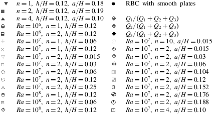


 Open access