


1. Introduction
Rotating cones in axial inflow are one of the simplified models for probing the transition phenomena in three-dimensional boundary layers developed on aero-engine-nose-cones, launch vehicle tips, turbo-machinery rotors, etc. Generally, the rotation destabilises the boundary layer on a rotating cone such that the disturbances grow to form coherent vortex structures close to the cone surface. In the presence of the meridional velocity component, the instability-induced vortices align in a spiral vortex pattern around the cone surface (Kobayashi & Izumi Reference Kobayashi and Izumi1983). As the azimuthal wall velocity increases with the radius, the spiral vortices grow and eventually set on the turbulence (Kohama Reference Kohama1984a). In practice, this transition phenomena, i.e. the spiral vortex growth and the turbulence onset, affect the performance of an engineering system – by altering the momentum distribution near the wall, affecting the local skin friction and heat transfer.
The cone rotation destabilises the boundary layer through two types of primary instabilities: centrifugal and cross-flow instabilities. The centrifugal instability relates to the balance between the centripetal force and the radial pressure gradient – inducing counter-rotating vortices on rotating cylinders (Taylor Reference Taylor1923; Hollerbach, Lueptow & Serre Reference Hollerbach, Lueptow and Serre2023), concave walls (Görtler Reference Görtler1954) and rotating cones with relatively small half-apex angle  $\psi \lesssim 30^\circ$ (Kobayashi, Kohama & Kurosawa Reference Kobayashi, Kohama and Kurosawa1983) in still fluid (Hussain, Stephen & Garrett Reference Hussain, Stephen and Garrett2012; Hussain, Garrett & Stephen Reference Hussain, Garrett and Stephen2014) and in axial flow (Hussain et al. Reference Hussain, Garrett, Stephen and Griffiths2016; Song & Dong Reference Song and Dong2023; Song, Dong & Zhao Reference Song, Dong and Zhao2023). The cross-flow instability arises from the inflectional meridional velocity profile – inducing co-rotating vortices, which have been investigated on rotating disks (Smith Reference Smith1947; Gregory, Stuart & Walker Reference Gregory, Stuart and Walker1955; Lingwood Reference Lingwood1995), on smooth rotating broad cones $\psi \gtrsim 30^\circ$ (Kobayashi & Izumi Reference Kobayashi and Izumi1983) within still fluid (Garrett, Hussain & Stephen Reference Garrett, Hussain and Stephen2009), axial flow (Garrett, Hussain & Stephen Reference Garrett, Hussain and Stephen2010) and, more recently, on rough rotating cones (Al-Malki, Fildes & Hussain Reference Al-Malki, Fildes and Hussain2022), as well as on swept wings (Kohama Reference Kohama2000).
Generally, a rotating-cone boundary layer undergoes transitions through three distinctly observable phases along the cone: (1) the critical phase where the instability-induced spiral vortices begin their growth, (2) the maximum amplification phase where the spiral vortex amplification peaks, where the vortices rapidly enhance mixing of the outer and inner flow, and (3) the turbulence onset phase where the velocity fluctuation spectra start resembling a general turbulence spectrum (Kobayashi et al. Reference Kobayashi, Kohama and Kurosawa1983; Kohama Reference Kohama1984b). The present article refers to these phases as transition points in geometric or flow-parameter spaces. In the transition region from the critical to turbulence onset, the instability-induced spiral vortices alter the thermal footprint and velocity distribution of the cone boundary layer. These effects are measurable and useful in identifying the phases of boundary-layer transition on rotating cones, as reported in the previous literature (Kobayashi et al. Reference Kobayashi, Kohama and Kurosawa1983, Reference Kobayashi, Kohama, Arai and Ukaku1987; Kato et al. Reference Kato, Segalini, Alfredsson and Lingwood2021; Tambe et al. Reference Tambe, Schrijer, Gangoli Rao and Veldhuis2021).
On a cone/disk rotating in still fluid, transition has been evaluated by a single parameter such as rotational Reynolds number based on the local radius and wall velocity (Kobayashi & Izumi Reference Kobayashi and Izumi1983; Lingwood Reference Lingwood1995, Reference Lingwood1996; Garrett et al. Reference Garrett, Hussain and Stephen2009; Hussain et al. Reference Hussain, Garrett and Stephen2014). Recently, Kato et al. (Reference Kato, Segalini, Alfredsson and Lingwood2021) suggested another parameter, Görtler number  $G$, and experimentally showed that thickening of the boundary layer due to transition can be scaled by Görtler number rather than the Reynolds number on a $\psi =30^\circ$ cone.
When the cone is rotating in axial inflow, however, both cone rotation and axial inflow are two independent control parameters. Therefore, Kobayashi et al. (Reference Kobayashi, Kohama and Kurosawa1983), Kobayashi et al. (Reference Kobayashi, Kohama, Arai and Ukaku1987) identified two flow parameters for scaling the boundary-layer transition on rotating cones in axial inflow: (1) the local rotational speed ratio  $S=r^*\varOmega ^*/U_e^*$ which accounts for the boundary-layer skew, and (2) the local Reynolds number $Re_l=l^*U_e^*/\nu ^*$ comparing the inertial vs viscous effects. Here, asterisk denotes dimensional variables; as schematically shown in figure 1, $r^*=l^*\sin \psi$ is the local cone radius, $l^*$ is the local meridional length from the cone apex, $\varOmega ^*$ is the angular velocity of the cone, $U_e^*$ is the meridional component of the boundary-layer edge velocity, $\nu ^*$ is the kinematic viscosity, $U^*_{\infty }$ is the free-stream velocity, $L^*$ is the total meridional length of a cone, and $U^*$, $V^*$ are the meridional and azimuthal velocity components.

Figure 1. Schematic of a rotating cone in axial inflow.
The present article reports the efficacy of Görtler-number-based scaling of the boundary-layer transition on rotating cones in axial inflow, which reduces the two-parameter scaling ( $Re_l$– $S$) down to a single parameter $G$. Section 2 describes the Görtler number and the basic flow formulation as functions of the local rotational speed ratio $S$, which inversely represents the axial inflow strength. Section 3 describes the experiments, in which the flow data were obtained. Section 4 presents the measured flow data and reported transition points along conventional $Re_l$– $S$ scale as well as along Görtler-number scale. Section 5 concludes the article.
2. Görtler number and the basic flow formulation
Görtler (Reference Görtler1954) showed that due to the centrifugal effects, a boundary layer on a concave wall becomes unstable and its instability induces counter-rotating vortices – also known as Görtler vortices. Furthermore, the vortices form at a constant Görtler number – which is a product of two non-dimensional parameters: Reynolds number comparing the inertial vs viscous effects and a curvature term  $\epsilon _c$ accounting for the wall-normal extent of the viscous effects, e.g. boundary-layer thickness compared with the radius of wall curvature (Taylor Reference Taylor1923; Görtler Reference Görtler1954; Saric Reference Saric1994).
On a rotating cone, the centrifugal effects exist because the viscous flow on the cone wall follows the curved motion of the rotating-cone surface. The curved flow within the boundary layer affects its instability behaviour which can be evaluated by Görtler number  $G$ formulated with the azimuthal-momentum-based Reynolds number $Re_{\delta ^*}=r^*\varOmega ^*\delta ^*/\nu ^*$ and the curvature term $\epsilon _c=\sqrt {\delta ^*/r^*}$:
 \begin{equation} G=Re_{\delta^*}\epsilon_{c}=\frac{r^*\varOmega^*\delta^*}{\nu^*} \sqrt{\frac{\delta^*}{r^*}}=\sqrt{\delta^3r}=\sqrt{\delta^3l \sin\psi}. \end{equation}
 Here,  $\varOmega ^*$ is the angular velocity and the azimuthal momentum thickness
 \begin{equation} \delta^*=\int_0^\infty V(1-V)\, {\rm d} z^*. \end{equation}
Here,  $V$ is the azimuthal velocity normalised by the local wall velocity $r^*\varOmega ^*$, $z^{*}$ is the wall-normal coordinate, $\delta =\delta ^*/\delta _\nu ^*$ is the azimuthal momentum thickness normalised by the length scale $\delta _\nu ^*=\sqrt {\nu ^*/\varOmega ^*}$, $r=r^*/\delta _\nu ^*$ and $l=l^*/\delta _\nu ^*$. Since the strongest curvature appears at the rotating cone surface, the local cone radius $r^*$ is chosen as the radius of curvature in $\epsilon _c$; and as the rotation adds momentum in the azimuthal direction, the azimuthal momentum thickness $\delta ^*$ accounts for the wall-normal extent of viscous effects in $\epsilon _c$.
For a fixed non-dimensional radius  $r$, Görtler number only depends on the non-dimensional azimuthal momentum thickness $\delta$ in (2.1). In the present work, we used the basic flow to compute $\delta$, assuming that the instability-induced distortion of the mean flow remains small until the maximum amplification phase, which will be validated through figures 4 and 5 in § 4. In the rest of this section, we describe the basic flow formulation and the effect of axial flow (or $S$) on $\delta$, which consequently affects the local Görtler number $G$ for a given $r$.
$r$.
The basic flow is computed using the formulation given in § 2.3 of Hussain (Reference Hussain2010), which is based on the formulation by Koh & Price (Reference Koh and Price1967). Following the Mangler transformation, Hussain used a stream-function-based similarity type transformation to obtain the governing equations in the non-dimensional form (Hussain Reference Hussain2010). The stream function
 \begin{equation} \varPsi= \left(\frac{m+3}{2s^{{1}/{2}}} \sin \psi \right)^{-{1}/{2}} f(s,\eta_1) \implies U^*=U_e^* \frac{\partial f(s,\eta_1)}{\partial \eta_1} \quad \text{and}\quad V^*=r^*\varOmega^*(g(s,\eta_1)+1). \end{equation}
Here,
 \begin{equation} s= S^2=\left( \frac{r^*\varOmega^*}{U_e^*} \right) ^2, \quad \eta_1=\eta \left( \frac{m+3}{2s^{{1}/{2}}}\sin \psi \right)^{{1}/{2}}, \end{equation} $\eta$ is the scaled wall-normal coordinate $z^*/\delta _\nu ^*$, $m$ is the exponent in the potential flow solution over a cone $U_e^*=C^*{l^*}^m$, where $C^*$ is a constant; for $\psi =15^\circ$, $30^\circ$, and $50^\circ$, $m=0.0396$, $0.117$ and $0.3$, respectively (Hussain Reference Hussain2010). The governing partial differential equations of the basic flow are as follows:
 $$\begin{gather} f''' +ff''+\frac{2m}{m+3}(1-f'^2)+\frac{2s}{m+3}\left[(g+1)^2+2(1-m)\left(\,f''\frac{\partial f}{\partial s}-f'\frac{\partial f'}{\partial s}\right)\right]=0, \end{gather}$$
 $$\begin{gather}g''+fg'-\frac{4}{m+3}f'(g+1)+\frac{4(1-m)s}{m+3}\left(g'\frac{\partial f}{\partial s} -f' \frac{\partial g}{\partial s} \right)=0. \end{gather}$$
 Here,  $'$ denotes the $\partial /\partial \eta _1$. The boundary conditions are
 \begin{equation} f=0, f'=0, g=0,\text{ on } \eta_1=0; \quad \textrm{and}\quad f' \rightarrow1, g\rightarrow-1, \text{ as } \eta_1 \rightarrow \infty. \end{equation}
A commercial routine NAG D03PEF is used to obtain the basic flow solution. Hussain et al. (Reference Hussain, Garrett, Stephen and Griffiths2016) have used this basic flow to successfully predict the trend of the critical Reynolds number for the instability onset on a rotating slender cone ( $\psi =15^\circ$) in axial inflow – agreeing with the experimental results (Kobayashi et al. Reference Kobayashi, Kohama and Kurosawa1983; Tambe et al. Reference Tambe, Schrijer, Gangoli Rao and Veldhuis2021), also shown in figure 6(a).
Figure 2 shows the computed velocity profiles of the basic flow for three different half-cone angles  $\psi =15^\circ$, $30^\circ$ and $50^\circ$. When the axial inflow is dominant over the rotation (e.g. figure 2a at $S=0.32$), the momentum is distributed in both azimuthal and meridional directions. However, when the rotation is dominant (e.g. figure 2b at $S=100$), most of the momentum is distributed in the azimuthal direction. Furthermore, the meridional velocity takes the inflectional form, owing to the increased meridional pressure gradient caused by the strong rotation.

Figure 2. Three-dimensional boundary-layer profiles on rotating cones ( $\psi =15^\circ$, $30^\circ$ and $50^\circ$) with examples of (a) strong axial inflow $S=0.32$ and (b) strong rotation $S=100$. (c) Variation of the azimuthal momentum thickness with the local rotational speed ratio $S$. Here $\delta _1$ is the momentum thickness in the transformed wall-normal coordinate $\eta _1$; $\delta$ is the momentum thickness in the scaled wall-normal coordinate $\eta =z^*/\delta _\nu ^*$.
Owing to the transformation (2.3a,b), the basic flow profiles for different half-cone angles  $\psi$ closely follow each other, especially in the azimuthal direction, see figures 2(a) and 2(b). Consequently, their azimuthal momentum thickness $\delta _1$ (in $\eta _1$ coordinates) follows a common trend with respect to the local rotational speed ratio $S$, see figure 2(c). This shows that varying axial inflow influences the wall-normal distribution of the azimuthal momentum. When transformed back onto the physical coordinates $\eta$, azimuthal momentum thickness $\delta$ increases with $S$ and decreases with the half-cone angle $\psi$. Thus, at a fixed non-dimensional radius $r$, increasing axial inflow strength or reducing $S$ will lower the local Görtler number $G$, weakening the centrifugal effects. This shows that the Görtler number formulation in (2.1) accounts for the axial flow strength (inverse of local rotational speed ratio $S$) through $\delta$.
3. Methodology
The efficacy of Görtler-number-based scaling for boundary-layer transition on rotating cones is assessed by using surface temperature fluctuations and the velocity fields obtained as described in Tambe (Reference Tambe2022) and by evaluating the Görtler numbers for the transition points reported along the two-parameter  $Re_l$– $S$ space in the literature. Parts of the raw data have been used to estimate the transition points reported by Tambe et al. (Reference Tambe, Schrijer, Gangoli Rao and Veldhuis2021, Reference Tambe, Schrijer, Gangoli Rao and Veldhuis2023).
The experiments were performed at a low-speed open jet wind tunnel (named  $W$-tunnel) at Aerospace Engineering, Delft University of Technology. The cones, made of polyoxymethylene (POM), were rotated in an axial inflow with the free-stream velocity $U_{\infty }^*=0.7\unicode{x2013}10.7\ {\rm m}\ {\rm s}^{-1}$ and typical turbulence level below $0.01U_{\infty }^*$. Infrared thermography (IRT) is performed at a frequency of $200$ Hz using an infrared camera FLIR (CEDIP) SC7300 Titanium to detect the thermal footprints of the instability-induced features, as described in Tambe et al. (Reference Tambe, Schrijer, Gangoli Rao and Veldhuis2019, Reference Tambe, Schrijer, Gangoli Rao and Veldhuis2021). Moreover, the meridional velocity field is measured with two-component particle image velocimetry (PIV) at a frequency of $2000$ Hz, using a high-speed camera Photron Fastcam SA-1 and a high-speed laser Nd:YAG Quantronix Darwin Duo 527-80-M. The flow is seeded with smoke particles having a mean diameter of approximately $1\ \mathrm {\mu }$m. Two-component velocity vector fields (with the vector pitch of approximately $2.6 \times 10^{-4}$ m) are obtained using a commercial software DaVis 8.4.0.
Cones with different half-cone angles  $\psi =15^\circ$, $30^\circ$ and $50^\circ$ are rotated at various rotational speeds (0–13 500 r.p.m.) to obtain different combinations of the operating conditions, i.e. $S_b=L^*\sin \psi \varOmega ^* /U_{\infty }^*$ and inflow Reynolds number $Re_L=L^*U_{\infty }^*/\nu ^*$. As $\delta$ varies with $S$ (figure 2c), the measurement uncertainties of $S$ and $l^*$ ( $\pm 0.06S$ and $\pm 0.02l^*$, respectively) cause uncertainty in Görtler number (using (2.1)) of approximately $\pm 0.1G$ .
4. Results and discussions
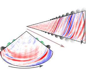
During the boundary-layer transition on a rotating cone in axial inflow, the growing spiral vortices increase the surface temperature fluctuations, which is detected using IRT (Tambe et al. Reference Tambe, Schrijer, Gangoli Rao and Veldhuis2019, Reference Tambe, Schrijer, Gangoli Rao and Veldhuis2021). Figure 3(a) shows the r.m.s. of surface temperature fluctuations along a cone with the half-cone angle  $\psi =15^\circ$ at different operating conditions, i.e. different combinations of base rotational speed ratio $S_b$ and inflow Reynolds number $Re_L$. The temperature fluctuations are in terms of the normalised pixel intensity $I'_{rms}/I'_{rms, max}$. Critical and maximum amplification phases of the spiral vortex growth are identified for all profiles; examples are marked in figure 3(a). Here, the critical points are the intersection points (marked by squares) of the baseline noise level and the least-square linear fit through the rising $I'_{rms}/I'_{rms, max}$, which represents the rapid growth of the spiral vortices. Further downstream, the growth saturates at the $I'_{rms}/I'_{rms, max}$ peak (the maximum amplification phase marked by the arrows), and, subsequently, the flow becomes turbulent (the turbulence onset phase) (Tambe et al. Reference Tambe, Schrijer, Gangoli Rao and Veldhuis2021, Reference Tambe, Schrijer, Gangoli Rao and Veldhuis2023). When the inflow Reynolds number $Re_L$ is increased at a fixed $\varOmega ^*$ (consequently, $S_b$ is decreased), the spiral vortex growth shifts downstream on the cone – showing that the scaled meridional length $l^*/\delta _\nu ^*$ does not scale the spiral vortex growth. In contrast, figure 3(b) shows that, on the Görtler number scale, the temperature fluctuation profiles associated with the spiral vortex growth overlap with each other. This confirms that Görtler number is an appropriate parameter for scaling the spiral vortex growth region on a rotating cone in axial inflow.

Figure 3. Meridional profiles of r.m.s. of surface temperature fluctuations ( $I'_{rms}/I'_{rms,max}$), caused by the growth of instability-induced spiral vortices on a rotating cone ( $\psi =15^\circ$), represented along (a) scaled meridional length $l^*/\delta _\nu ^*$ and (b) Görtler number scale. Squares and downward arrows represent the critical and maximum amplification points, respectively.
The amplified spiral vortices begin to interact with the outer flow and enhance mixing; the enhanced mixing starts to increase the boundary layer thickness. For example, figures 4(a) and 4(b), show the mean meridional velocity fields over a rotating cone ( $\psi =15^\circ$) on the local Reynolds number scale, at two different operating conditions. Here, the black dashed line marks the location of maximum amplification identified from the surface temperature fluctuations (e.g. figure 3). The solid and dotted black lines represent the boundary-layer thicknesses $\delta _{95,{exp}}$ and $\delta _{95,{th}}$ obtained from the measured mean flow and computed basic flow, respectively; $\delta _{95}$ is the wall-normal extent along $\eta$ up to which the meridional velocity deficit (or excess, e.g. at high $S$, figure 2b) is more than $5\,\%$ of the outer irrotational flow velocity. Before the maximum amplification, the measured boundary-layer thickness (solid line) follows that of the basic flow (dotted line) within $0.1\unicode{x2013}0.2 \delta _{95,{exp}}$ but starts to drastically deviate around the maximum amplification. The velocity fields in two different cases, as shown in the left columns of figures 4(a) and 4(b), do not align with each other on the local Reynolds number $Re_l$ scale – suggesting that $Re_l$ alone is not an appropriate scaling parameter for the rotating cones. However, on the Görtler number scale, the near-wall velocity fields and the maximum amplification locations align close to each other at $G\approx 7.5$, as shown in the right columns. This further confirms that the Görtler number appropriately scales the spiral vortex growth region on a rotating slender cone $\psi =15^\circ$.

Figure 4. Mean meridional velocity field obtained from PIV over a rotating cone of  $\psi =15^\circ$ on Reynolds number and Görtler number scales with (a) $S_b=1.9$ and $Re_L=9.7 \times 10^4$; (b) $S_b=3.1$ and $Re_L=6.2 \times 10^4$. Solid and dotted black lines represent the boundary-layer thicknesses $\delta _{95,{exp}}$ and $\delta _{95,{th}}$ obtained from measured mean flow and computed basic flow, respectively. The black dashed line represents the maximum amplification identified from surface temperature fluctuations.
Generally, increasing the half-cone angle has a stabilising effect on the boundary layer, such that the transition is delayed to higher values of local Reynolds number  $Re_l$ and local rotational speed ratio $S$ (Kobayashi et al. Reference Kobayashi, Kohama, Arai and Ukaku1987; Garrett et al. Reference Garrett, Hussain and Stephen2010; Tambe et al. Reference Tambe, Schrijer, Gangoli Rao and Veldhuis2023). For example, at a fixed local Reynolds number ( $Re_l$), broader cones require a stronger rotation effect (higher $S$) to cause the boundary-layer transition. Figure 5 shows the mean velocity fields for two rotating cones ( $\psi =30^\circ$ and $50^\circ$, respectively) on $Re_l$ and $G$ scales. Due to the high rotation rates, typically $S \gtrsim 5$, the local meridional velocity is higher as compared with the boundary-layer edge (e.g. as also seen in figure 2b). Similar to $\psi =15^\circ$ (figure 4), on broad cones $\psi =30^\circ$ and $50^\circ$ (figure 5), the measured boundary-layer thickness (solid white line) is close to that of the basic flow (dotted white line) within $0.1\unicode{x2013}0.2 \delta _{95,{exp}}$ until the maximum amplification, beyond which it increases. For both these cones, the velocity fields align with each other on the Görtler number scale, unlike on the local Reynolds number scale. This shows that the Görtler-number-based scaling is effective for a range of half-cone angles: from slender ( $\psi =15^\circ$) to broad ( $\psi =50^\circ$) cones. The Görtler number related to the maximum amplification increases from approximately $G\approx 7.5$ for a slender cone $\psi =15^\circ$ to approximately $G\approx 10\unicode{x2013}11$ for the broader cones $\psi =3 0^\circ$ and $50^\circ$.

Figure 5. Mean meridional velocity field obtained from PIV over a rotating cone of (a–c)  $\psi =30^\circ$ and (d–f) $50^\circ$ on Reynolds number and Görtler number with (a) $S_b=28.4$, $Re_L=8 \times 10^3$; (b) $S_b=15.7$, $Re_L=1.5 \times 10^4$; (c) $S_b=10.8$, $Re_L=2.2 \times 10^4$; (d) $S_b=94$, $Re_L=3 \times 10^3$; (e) $S_b=55.6$, $Re_L=5\times 10^3$; (f) $S_b=18.0$, $Re_L=1.7\times 10^4$. Solid and dotted white lines represent the boundary-layer thicknesses $\delta _{95,{exp}}$ and $\delta _{95,{th}}$ obtained from measured mean flow and computed basic flow, respectively. The black dashed line represents the maximum amplification identified from surface temperature fluctuations.
To assess the generality of Görtler-number-based scaling of rotating-cone boundary-layer transition, Görtler numbers are evaluated for the transition points reported by different studies in the literature in  $Re_l$– $S$ parameter space, which used different wind tunnel facilities, different model sizes (base diameters $D^*=L^*\sin \psi =0.047\unicode{x2013}0.1$m), different measurement techniques (hot-wire anemometry, infrared thermography, etc.), transition criteria, free-stream turbulence levels ( $0.05\unicode{x2013}1\,\%$), half-cone angles ( $\psi =15^\circ$, $30^\circ$ and $50^\circ$) (Kobayashi & Izumi Reference Kobayashi and Izumi1983; Kobayashi et al. Reference Kobayashi, Kohama and Kurosawa1983, Reference Kobayashi, Kohama, Arai and Ukaku1987; Tambe et al. Reference Tambe, Schrijer, Gangoli Rao and Veldhuis2021, Reference Tambe, Schrijer, Gangoli Rao and Veldhuis2023) and theoretical analysis (Hussain et al. Reference Hussain, Garrett, Stephen and Griffiths2016). The transition points (relating to critical, maximum amplification and turbulence onset phases) are shown in $Re_l$– $S$ space directly as they are reported in the literature (figure 6a–c) and, after estimating their respective Görtler numbers, they are represented in $G$–
$G$– $S$ space (figure 6d–f, transformed using (2.1), where $\delta$ is obtained from the similarity solution as shown in figure 2c and $l=\sqrt {Re_l S /\sin \psi }$). In $Re_l$– $S$ space (figures 6a–c), all transition points show a nearly log-linear behaviour. For a $\psi =15^\circ$ cone (figure 6a), a good agreement between theory and different measurements is shown, confirming that $Re_l$ and $S$ together are appropriate to represent the boundary-layer transition region on rotating cones. However, in $G$–
$G$– $S$ space (figure 6d for $\psi =15^\circ$), the transition points appear at respectively fixed Görtler numbers – regardless of the local rotational speed ratio in the investigated range $S\gtrsim 1$. The Görtler numbers for the measured turbulence onset points by Kobayashi et al. (Reference Kobayashi, Kohama, Arai and Ukaku1987) in axial inflow $S\approx 2.5\unicode{x2013}4.5$ agree with that of Kobayashi & Izumi (Reference Kobayashi and Izumi1983) in still fluid $S\approx \infty$ – both studies used the same measurement technique. Moreover, the critical points predicted by Hussain et al. (Reference Hussain, Garrett, Stephen and Griffiths2016) also appear within a narrow range of Görtler numbers. Considering the small variation of the respective Görtler numbers relative to the uncertainty of approximately $\pm 0.1G$, we can conclude that the critical and the maximum amplification points as well as turbulence onset on the rotating $15^\circ$ cone are scaled by Görtler number regardless of the axial inflow for $S \gtrsim 1$. At low local rotational speed ratio, i.e. $S \ll 1$, the centrifugal effects are expected to be weak and different mechanisms dominate transition (Song et al. Reference Song, Dong and Zhao2023). However, at $S \gtrsim 1$, the centrifugal instability is known to be dominant on the slender cone (Kobayashi & Izumi Reference Kobayashi and Izumi1983; Kobayashi et al. Reference Kobayashi, Kohama and Kurosawa1983; Hussain et al. Reference Hussain, Garrett, Stephen and Griffiths2016; Kato et al. Reference Kato, Segalini, Alfredsson and Lingwood2021), and the influence of $S$ on Görtler number is reported here for the first time. Thus, when the transition is induced due to the strong rotation effect ( $S \gtrsim 1$), Görtler number is an appropriate parameter to scale the boundary-layer transition on a rotating slender cone $\psi =15^\circ$ rather than using the two-parameter space $Re_l$– $S$.
$S$.

Figure 6. The boundary-layer transition on rotating cones ((a,d)  $\psi =15^\circ$, (b,e) $\psi =30^\circ$ and (c,f) $\psi =50^\circ$) in two different parameter spaces: (a–c) Reynolds number and local rotational speed ratio ( $Re_l$– $S$) as reported in the literature, and (d–f) the estimated Görtler number and local rotational speed ratio ( $G$–
$G$– $S$).
$S$).
For broader cones  $\psi =30^\circ$ and $50^\circ$, figures 6(e) and 6(f) show the transition points in $G$–
$G$– $S$ space, respectively. Unlike their near-log-linear trends in the $Re_l$– $S$ space (figures 6b and 6c), the maximum amplification and turbulence onset points in $G$–
$G$– $S$ space appear in a narrow Görtler number range for the investigated values of $S$. Moreover, maximum amplification points for both the cones ( $\psi =30^\circ$ and $50^\circ$) appear in the range $G\approx 10\unicode{x2013}11$ as shown in figures 5, 6(e) and 6(f). This range agrees with the results of Kato et al. (Reference Kato, Segalini, Alfredsson and Lingwood2021) on a $\psi =30^\circ$ cone rotating in still fluid ( $S\approx \infty$), although there are some differences in the transition criteria and the way of calculating the momentum thickness; Kato et al. (Reference Kato, Segalini, Alfredsson and Lingwood2021) reported a gradual thickening of the boundary layer, starting at approximately $G=10$ based on the measured momentum thickness evaluated below the $90\,\%$ boundary-layer thickness whereas the present $\delta$ is obtained by integrating the similarity solution in the infinite space. Moreover, the turbulence onset points for $\psi =30^\circ$ cone appear at $G=10\unicode{x2013}12$ (figure 6e). Thus, the maximum amplification point, beyond which the measured mean flow drastically deviates from the similarity solution flow, and turbulent onset occur in a well-defined range of Görtler numbers for a wide range of investigated $S$. However, the critical points vary with respect to the local rotational speed ratio $S$ in $G$–
$G$– $S$ space at high rotational speed ratio $S\gtrsim 5$ (figures 6e and 6f), where, for broader cones $\psi \geq 30^\circ$, the primary cross-flow instability dominates the flow rather than centrifugal instability (Kobayashi & Izumi Reference Kobayashi and Izumi1983; Kobayashi et al. Reference Kobayashi, Kohama, Arai and Ukaku1987; Garrett et al. Reference Garrett, Hussain and Stephen2010).
It is interesting that Görtler number dominates the maximum amplification and turbulence onset on broader cones  $\psi =30^\circ$ and $50^\circ$ at higher $S \gtrsim 5$ (figures 5, 6e and 6f), where the primary instability is the cross-flow instability and forms co-rotating primary vortices. A possible explanation for this might be that the centrifugal effects cause a secondary instability; some measurements, e.g. figure 7 from Tambe et al. (Reference Tambe, Schrijer, Gangoli Rao and Veldhuis2023) and also the top right of figure 8b from Kobayashi & Izumi (Reference Kobayashi and Izumi1983), show that new counter-rotating vortices emerge near the maximum amplification (after the primary co-rotating vortices have developed), which might be caused by centrifugal effects. Dominance of Görtler number in this region suggests that the centrifugal effects play an important role in the spiral vortex amplification and turbulence onset even on the broad cones where the cross-flow primary instability dominates the flow initially.
5. Conclusion
The Görtler number is found to scale the centrifugal instability-led boundary-layer transition on a rotating slender cone ( $\psi =15^\circ$) in axial inflow. For the local rotational speed ratio $S \gtrsim 1$, the critical, maximum amplification and turbulence onset points appear at well-defined Görtler numbers respectively, regardless of the axial inflow strength or local rotational speed ratio $S$. Therefore, the Görtler number alleviates the need to use the conventional two-parameter space of local Reynolds number $Re_l$ and local rotational speed ratio $S$ to represent the transition points on a rotating slender cone ( $\psi =15^\circ$) in axial inflow for $S \gtrsim 1$.
On broader cones  $\psi =30^\circ$ and $50^\circ$, where the cross-flow instability is the dominant primary instability, the maximum amplification and turbulence onset are found to occur at approximately $G=10\unicode{x2013}12$ which is affected marginally by $S$, although the critical Görtler number varies with $S$. This suggests that, for $S \gtrsim 1$, the centrifugal effects play an important role in boundary-layer transition for a wide range of investigated rotating cones with $15^{\circ } \leq \psi \leq 50^{\circ }$, regardless of the axial inflow. Further investigation is required to understand the detailed role of the centrifugal effects in the turbulence onset mechanism.
Acknowledgements
Authors wish to acknowledge F. Schrijer, A. Gangoli Rao, L. Veldhuis, and TU Delft Wind Tunnel Labs for the experimental data.
Funding
S. Tambe acknowledges the fellowship support of the Department of Science and Technology, Government of India for this work and the European Union Horizon 2020 program: Clean Sky 2 Large Passenger Aircraft (CS2-LPA-GAM-2018-2019-01) and CENTERLINE (grant agreement No. 723242) for the experimental data. K. Kato acknowledges support from JSPS KAKENHI grant number JP22K20406.
Declaration of interests
The authors report no conflict of interest.
Data availability statement
Data are available upon a reasonable request.
Author contributions
S. Tambe contributed to measuring and analysing data, conceptualising and writing the first draft manuscript. K. Kato contributed to conceptualising and writing the manuscript. Z. Hussain contributed to basic flow computation, conceptualising and writing the manuscript.


 Open access