

1 The problem
The upper bound derived in Kerswell (Reference Kerswell2016) is incorrect. This is because the $I_{4}$
and
$I_{4}$
and $I_{5}$
integrals centred at the top boundary are not exactly analogous to their counterparts at the lower boundary, counter to what is written just under equation (2.23) (in Kerswell Reference Kerswell2016). Instead, in both cases, due to the roughness, the full volume integrals must be included which scale differently with
$I_{5}$
integrals centred at the top boundary are not exactly analogous to their counterparts at the lower boundary, counter to what is written just under equation (2.23) (in Kerswell Reference Kerswell2016). Instead, in both cases, due to the roughness, the full volume integrals must be included which scale differently with $\ell$
. Specifically, the estimates for the
$\ell$
. Specifically, the estimates for the $I_{4}$
and
$I_{4}$
and $I_{5}$
integrals centred at the top boundary are
$I_{5}$
integrals centred at the top boundary are
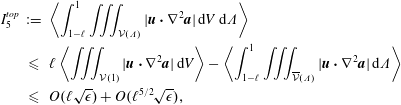 $$\begin{eqnarray}\displaystyle I_{5}^{top} & := & \displaystyle \left\langle \int _{1-\ell }^{1}\iiint _{{\mathcal{V}}(\unicode[STIX]{x1D6EC})}|\boldsymbol{u}\boldsymbol{\cdot }\unicode[STIX]{x1D6FB}^{2}\boldsymbol{a}|\,\text{d}V\,\text{d}\unicode[STIX]{x1D6EC}\right\rangle \nonumber\\ \displaystyle & {\leqslant} & \displaystyle \ell \left\langle \iiint _{{\mathcal{V}}(1)}|\boldsymbol{u}\boldsymbol{\cdot }\unicode[STIX]{x1D6FB}^{2}\boldsymbol{a}|\,\text{d}V\right\rangle -\left\langle \int _{1-\ell }^{1}\iiint _{\overline{{\mathcal{V}}}(\unicode[STIX]{x1D6EC})}|\boldsymbol{u}\boldsymbol{\cdot }\unicode[STIX]{x1D6FB}^{2}\boldsymbol{a}|\,\text{d}\unicode[STIX]{x1D6EC}\right\rangle \nonumber\\ \displaystyle & {\leqslant} & \displaystyle O(\ell \sqrt{\unicode[STIX]{x1D716}})+O(\ell ^{5/2}\sqrt{\unicode[STIX]{x1D716}}),\nonumber\end{eqnarray}$$
where $\overline{{\mathcal{V}}}(\unicode[STIX]{x1D6EC}):={\mathcal{V}}(1)-{\mathcal{V}}(\unicode[STIX]{x1D6EC})$
so the last term can be estimated as in expression (2.23), and
$\overline{{\mathcal{V}}}(\unicode[STIX]{x1D6EC}):={\mathcal{V}}(1)-{\mathcal{V}}(\unicode[STIX]{x1D6EC})$
so the last term can be estimated as in expression (2.23), and
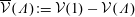
 $$\begin{eqnarray}\displaystyle I_{4}^{top} & := & \displaystyle \left\langle \int _{1-\ell }^{1}\iiint _{{\mathcal{V}}(\unicode[STIX]{x1D6EC})}|\boldsymbol{u}\boldsymbol{\cdot }(\boldsymbol{u}\boldsymbol{\cdot }\unicode[STIX]{x1D735})\boldsymbol{a}|\,\text{d}V\,\text{d}\unicode[STIX]{x1D6EC}\right\rangle \nonumber\\ \displaystyle & {\leqslant} & \displaystyle \ell \left\langle \iiint _{{\mathcal{V}}(1)}|\boldsymbol{u}\boldsymbol{\cdot }(\boldsymbol{u}\boldsymbol{\cdot }\unicode[STIX]{x1D735})\boldsymbol{a}|\,\text{d}V\right\rangle -\left\langle \int _{1-\ell }^{1}\iiint _{\overline{{\mathcal{V}}}(\unicode[STIX]{x1D6EC})}|\boldsymbol{u}\boldsymbol{\cdot }(\boldsymbol{u}\boldsymbol{\cdot }\unicode[STIX]{x1D735})\boldsymbol{a}|\,\text{d}\unicode[STIX]{x1D6EC}\right\rangle \nonumber\\ \displaystyle & {\leqslant} & \displaystyle O(\ell \unicode[STIX]{x1D716})+O(\ell ^{3}\unicode[STIX]{x1D716}),\nonumber\end{eqnarray}$$
where again the last term can be estimated as in expression (2.22). The first term of $O(\ell \unicode[STIX]{x1D716})$
on the right-hand side in this modified estimate of
$O(\ell \unicode[STIX]{x1D716})$
on the right-hand side in this modified estimate of $I_{4}^{top}$
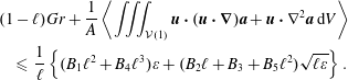
is the key new addition which breaks the bound. To see this, it is best to start with equation (2.16) rearranged slightly as follows
$I_{4}^{top}$
is the key new addition which breaks the bound. To see this, it is best to start with equation (2.16) rearranged slightly as follows
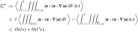
 $$\begin{eqnarray}\displaystyle & & \displaystyle (1-\ell )Gr+\frac{1}{A}\left\langle \iiint _{{\mathcal{V}}(1)}\boldsymbol{u}\boldsymbol{\cdot }(\boldsymbol{u}\boldsymbol{\cdot }\unicode[STIX]{x1D735})\boldsymbol{a}+\boldsymbol{u}\boldsymbol{\cdot }\unicode[STIX]{x1D6FB}^{2}\boldsymbol{a}\,\text{d}V\right\rangle \nonumber\\ \displaystyle & & \displaystyle \quad =\frac{1}{A}\left\langle \frac{1}{\ell }\int _{1-\ell }^{1}\int _{{\mathcal{S}}(\unicode[STIX]{x1D6EC})}(\boldsymbol{a}\boldsymbol{\cdot }\boldsymbol{u})\boldsymbol{u}\boldsymbol{\cdot }\hat{\boldsymbol{n}}+\boldsymbol{u}\boldsymbol{\cdot }(\hat{\boldsymbol{n}}\boldsymbol{\cdot }\unicode[STIX]{x1D735})\boldsymbol{a}-\boldsymbol{a}\boldsymbol{\cdot }(\hat{\boldsymbol{n}}\boldsymbol{\cdot }\unicode[STIX]{x1D735})\boldsymbol{u}\,\text{d}S\,\text{d}\unicode[STIX]{x1D6EC}\right.\nonumber\\ \displaystyle & & \displaystyle \qquad -\,\frac{1}{\ell }\int _{0}^{\ell }\int _{{\mathcal{S}}(\unicode[STIX]{x1D6EC})}(\boldsymbol{a}\boldsymbol{\cdot }\boldsymbol{u})\boldsymbol{u}\boldsymbol{\cdot }\hat{\boldsymbol{n}}+\boldsymbol{u}\boldsymbol{\cdot }(\hat{\boldsymbol{n}}\boldsymbol{\cdot }\unicode[STIX]{x1D735})\boldsymbol{a}-\boldsymbol{a}\boldsymbol{\cdot }(\hat{\boldsymbol{n}}\boldsymbol{\cdot }\unicode[STIX]{x1D735})\boldsymbol{u}\,\text{d}S\,\text{d}\unicode[STIX]{x1D6EC}\nonumber\\ \displaystyle & & \displaystyle \qquad +\,\frac{1}{\ell }\int _{1-\ell }^{1}\iiint _{\overline{{\mathcal{V}}}(\unicode[STIX]{x1D6EC})}\boldsymbol{u}\boldsymbol{\cdot }(\boldsymbol{u}\boldsymbol{\cdot }\unicode[STIX]{x1D735})\boldsymbol{a}+\boldsymbol{u}\boldsymbol{\cdot }\unicode[STIX]{x1D6FB}^{2}\boldsymbol{a}\,\text{d}V\,\text{d}\unicode[STIX]{x1D6EC}\nonumber\\ \displaystyle & & \displaystyle \qquad +\,\left.\frac{1}{\ell }\int _{0}^{\ell }\iiint _{{\mathcal{V}}(\unicode[STIX]{x1D6EC})}\boldsymbol{u}\boldsymbol{\cdot }(\boldsymbol{u}\boldsymbol{\cdot }\unicode[STIX]{x1D735})\boldsymbol{a}+\boldsymbol{u}\boldsymbol{\cdot }\unicode[STIX]{x1D6FB}^{2}\boldsymbol{a}\,\text{d}V\,\text{d}\unicode[STIX]{x1D6EC}\right\rangle\end{eqnarray}$$
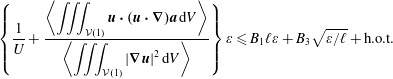
to highlight the full volume integrals present (now on the left). Then the arguments presented in the paper are correct to reach (2.24) which now reads
 $$\begin{eqnarray}\displaystyle & & \displaystyle (1-\ell )Gr+\frac{1}{A}\left\langle \iiint _{{\mathcal{V}}(1)}\boldsymbol{u}\boldsymbol{\cdot }(\boldsymbol{u}\boldsymbol{\cdot }\unicode[STIX]{x1D735})\boldsymbol{a}+\boldsymbol{u}\boldsymbol{\cdot }\unicode[STIX]{x1D6FB}^{2}\boldsymbol{a}\,\text{d}V\right\rangle \nonumber\\ \displaystyle & & \displaystyle \quad \leqslant \,\frac{1}{\ell }\left\{(B_{1}\ell ^{2}+B_{4}\ell ^{3})\unicode[STIX]{x1D700}+(B_{2}\ell +B_{3}+B_{5}\ell ^{2})\sqrt{\ell \unicode[STIX]{x1D700}}\right\}.\end{eqnarray}$$
For $\ell \rightarrow 0$
, this is (using the fact that
$\ell \rightarrow 0$
, this is (using the fact that $Gr=\unicode[STIX]{x1D700}/U$
)
$Gr=\unicode[STIX]{x1D700}/U$
)
 $$\begin{eqnarray}\left\{\frac{1}{U}+\frac{\left\langle \displaystyle \iiint _{{\mathcal{V}}(1)}\boldsymbol{u}\boldsymbol{\cdot }(\boldsymbol{u}\boldsymbol{\cdot }\unicode[STIX]{x1D735})\boldsymbol{a}\,\text{d}V\right\rangle }{\left\langle \displaystyle \iiint _{{\mathcal{V}}(1)}|\unicode[STIX]{x1D735}\boldsymbol{u}|^{2}\,\text{d}V\right\rangle }\right\}\unicode[STIX]{x1D700}\leqslant B_{1}\ell \unicode[STIX]{x1D700}+B_{3}\sqrt{\unicode[STIX]{x1D700}/\ell }+\text{h.o.t.}\end{eqnarray}$$
since
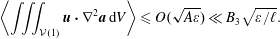 $$\begin{eqnarray}\left\langle \iiint _{{\mathcal{V}}(1)}\boldsymbol{u}\boldsymbol{\cdot }\unicode[STIX]{x1D6FB}^{2}\boldsymbol{a}\,\text{d}V\right\rangle \leqslant O(\sqrt{A\unicode[STIX]{x1D700}})\ll B_{3}\sqrt{\unicode[STIX]{x1D700}/\ell }.\end{eqnarray}$$
The right-hand side is minimised as before by $\ell =\unicode[STIX]{x1D700}^{-1/3}$
so that
$\ell =\unicode[STIX]{x1D700}^{-1/3}$
so that
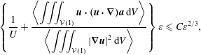 $$\begin{eqnarray}\left\{\frac{1}{U}+\frac{\left\langle \displaystyle \iiint _{{\mathcal{V}}(1)}\boldsymbol{u}\boldsymbol{\cdot }(\boldsymbol{u}\boldsymbol{\cdot }\unicode[STIX]{x1D735})\boldsymbol{a}\,\text{d}V\right\rangle }{\left\langle \displaystyle \iiint _{{\mathcal{V}}(1)}|\unicode[STIX]{x1D735}\boldsymbol{u}|^{2}\,\text{d}V\right\rangle }\right\}\unicode[STIX]{x1D700}\leqslant C\unicode[STIX]{x1D700}^{2/3},\end{eqnarray}$$
where $C$
is an
$C$
is an $O(1)$
constant or rewriting
$O(1)$
constant or rewriting
 $$\begin{eqnarray}\unicode[STIX]{x1D700}\leqslant C^{3}U^{3}\left/\left\{1+\frac{U\left\langle \displaystyle \iiint _{{\mathcal{V}}(1)}\boldsymbol{u}\boldsymbol{\cdot }(\boldsymbol{u}\boldsymbol{\cdot }\unicode[STIX]{x1D735})\boldsymbol{a}\,\text{d}V\right\rangle }{\left\langle \displaystyle \iiint _{{\mathcal{V}}(1)}|\unicode[STIX]{x1D735}\boldsymbol{u}|^{2}\,\text{d}V\right\rangle }\right\}^{3}\right..\end{eqnarray}$$
Since no lower bound is available on the denominator, this does not provide a bound on $\unicode[STIX]{x1D700}$
. In fact, the better way to view (1.5) is that it presents an upper bound on the denominator
$\unicode[STIX]{x1D700}$
. In fact, the better way to view (1.5) is that it presents an upper bound on the denominator
 $$\begin{eqnarray}\left\{1+\frac{U\left\langle \displaystyle \iiint _{{\mathcal{V}}(1)}\boldsymbol{u}\boldsymbol{\cdot }(\boldsymbol{u}\boldsymbol{\cdot }\unicode[STIX]{x1D735})\boldsymbol{a}\,\text{d}V\right\rangle }{\left\langle \displaystyle \iiint _{{\mathcal{V}}(1)}|\unicode[STIX]{x1D735}\boldsymbol{u}|^{2}\,\text{d}V\right\rangle }\right\}\leqslant O(U\unicode[STIX]{x1D700}^{-1/3})\end{eqnarray}$$
rather than a bound on $\unicode[STIX]{x1D700}$
.
$\unicode[STIX]{x1D700}$
.
2 Why there is no quick fix
It became apparent that there must be a problem with the bound in Kerswell (Reference Kerswell2016) when a connection was very recently made (Chernyshenko Reference Chernyshenko2017) between the ‘boundary layer’ method of Otto & Seis (Seis Reference Seis2015) and the background method (Doering & Constantin Reference Doering and Constantin1994). It is worthwhile illustrating this connection in the simpler context of the smooth-walled channel flow problem before giving the background velocity field corresponding to the Otto–Seis ‘boundary layer’ bounding analysis presented in Kerswell (Reference Kerswell2016). This background field has shears throughout the interior and so cannot ever satisfy the spectral constraint necessary to get a bound in the background approach. This, unfortunately, makes it clear that there is no simple fix of the flawed bound in Kerswell (Reference Kerswell2016).
We adopt Seis’s (Reference Seis2015) notation (see his § 4) so that if
 $$\begin{eqnarray}(\boldsymbol{N}\boldsymbol{S}):=\frac{\unicode[STIX]{x2202}\boldsymbol{u}}{\unicode[STIX]{x2202}t}+\boldsymbol{u}\boldsymbol{\cdot }\unicode[STIX]{x1D735}\boldsymbol{u}+\unicode[STIX]{x1D735}p-\unicode[STIX]{x1D6FB}^{2}\boldsymbol{u}-Gr\hat{\boldsymbol{x}}\end{eqnarray}$$
then $(\boldsymbol{N}\boldsymbol{S})=\mathbf{0}$
and
$(\boldsymbol{N}\boldsymbol{S})=\mathbf{0}$
and $\unicode[STIX]{x1D735}\boldsymbol{\cdot }\boldsymbol{u}=0$
with
$\unicode[STIX]{x1D735}\boldsymbol{\cdot }\boldsymbol{u}=0$
with $\boldsymbol{u}(x,y,0)=\boldsymbol{u}(x,y,1)=\mathbf{0}$
define the channel flow problem.
$\boldsymbol{u}(x,y,0)=\boldsymbol{u}(x,y,1)=\mathbf{0}$
define the channel flow problem.
2.1 The background method
The background method is to construct the functional
 $$\begin{eqnarray}{\mathcal{L}}[\boldsymbol{u},\unicode[STIX]{x1D742}]:=\left\langle \int _{0}^{1}\overline{|\unicode[STIX]{x1D735}\boldsymbol{u}|^{2}}\,\text{d}z\right\rangle -\unicode[STIX]{x1D6FC}\left\langle \int _{0}^{1}\overline{\unicode[STIX]{x1D742}\boldsymbol{\cdot }(\boldsymbol{N}\boldsymbol{S})}\,\text{d}z\right\rangle ,\end{eqnarray}$$
where $\unicode[STIX]{x1D6FC}$
is a balance (scalar) parameter (usually ‘a’ in past work),
$\unicode[STIX]{x1D6FC}$
is a balance (scalar) parameter (usually ‘a’ in past work), $\unicode[STIX]{x1D742}(\boldsymbol{x},t)$
is a Lagrange multiplier field and
$\unicode[STIX]{x1D742}(\boldsymbol{x},t)$
is a Lagrange multiplier field and
 $$\begin{eqnarray}\overline{(\cdot )}:=\frac{1}{L_{x}L_{y}}\int _{0}^{L_{x}}\int _{0}^{L_{y}}(\cdot )\,\text{d}y\,\text{d}x\end{eqnarray}$$
is an average over the rectangle $(x,y)\in [0,L_{x}]\times [0,L_{y}]$
. The key step is to restrict the difference between
$(x,y)\in [0,L_{x}]\times [0,L_{y}]$
. The key step is to restrict the difference between $\boldsymbol{u}$
and
$\boldsymbol{u}$
and $\unicode[STIX]{x1D742}$
by defining a background field
$\unicode[STIX]{x1D742}$
by defining a background field $\unicode[STIX]{x1D719}(z)$
such that
$\unicode[STIX]{x1D719}(z)$
such that
 $$\begin{eqnarray}\boldsymbol{u}(\boldsymbol{x},t)=\unicode[STIX]{x1D719}(z)\hat{\boldsymbol{x}}+\unicode[STIX]{x1D742}(\boldsymbol{x},t),\end{eqnarray}$$
where $\unicode[STIX]{x1D719}$
carries the mass flux of the flow but vanishes at the boundaries. In particular, if the energy dissipation rate is sought in terms of the mean flow
$\unicode[STIX]{x1D719}$
carries the mass flux of the flow but vanishes at the boundaries. In particular, if the energy dissipation rate is sought in terms of the mean flow $U$
rather than the imposed pressure gradient (
$U$
rather than the imposed pressure gradient ( $Gr$
) then
$Gr$
) then
 $$\begin{eqnarray}U:=\int _{0}^{1}\overline{\boldsymbol{u}\boldsymbol{\cdot }\hat{\boldsymbol{x}}}\,\text{d}z=\int _{0}^{1}\unicode[STIX]{x1D719}\,\text{d}z\end{eqnarray}$$
(see (2.29), Kerswell Reference Kerswell2016). Rewriting ${\mathcal{L}}$
in terms of
${\mathcal{L}}$
in terms of $\unicode[STIX]{x1D742}$
and
$\unicode[STIX]{x1D742}$
and $\unicode[STIX]{x1D719}$
, and then integrating by parts, the boundedness of the kinetic energy and the fact that both
$\unicode[STIX]{x1D719}$
, and then integrating by parts, the boundedness of the kinetic energy and the fact that both $\unicode[STIX]{x1D719}$
and
$\unicode[STIX]{x1D719}$
and $\unicode[STIX]{x1D742}$
vanish on
$\unicode[STIX]{x1D742}$
vanish on $z=0$
and
$z=0$
and $1$
leads to the simplified expression
$1$
leads to the simplified expression
 $$\begin{eqnarray}{\mathcal{L}}[\unicode[STIX]{x1D742},\unicode[STIX]{x1D719}]=\int _{0}^{1}\unicode[STIX]{x1D719}^{\prime 2}\,\text{d}z-\langle {\mathcal{G}}(\unicode[STIX]{x1D742};\unicode[STIX]{x1D719},\unicode[STIX]{x1D6FC})\rangle ,\end{eqnarray}$$
where
 $$\begin{eqnarray}{\mathcal{G}}:=\int _{0}^{1}(\unicode[STIX]{x1D6FC}-1)\overline{|\unicode[STIX]{x1D735}\unicode[STIX]{x1D742}|^{2}}+\overline{\unicode[STIX]{x1D6FC}\unicode[STIX]{x1D708}_{1}\unicode[STIX]{x1D708}_{3}\unicode[STIX]{x1D719}^{\prime }}-(\unicode[STIX]{x1D6FC}-2)\overline{\unicode[STIX]{x1D708}_{1}\unicode[STIX]{x1D719}^{\prime \prime }}\,\text{d}z.\end{eqnarray}$$
Then the background method (Doering & Constantin Reference Doering and Constantin1994) is the observation that
 $$\begin{eqnarray}{\mathcal{L}}\leqslant \int _{0}^{1}\unicode[STIX]{x1D719}^{\prime 2}\,\text{d}z-\min _{\unicode[STIX]{x1D742}}{\mathcal{G}}(\unicode[STIX]{x1D742};\unicode[STIX]{x1D719},\unicode[STIX]{x1D6FC}),\end{eqnarray}$$
where only steady fields now need to be considered. The important point is $\min {\mathcal{G}}$
only exists for
$\min {\mathcal{G}}$
only exists for $\unicode[STIX]{x1D6FC}>1$
and
$\unicode[STIX]{x1D6FC}>1$
and $\unicode[STIX]{x1D719}$
which satisfy the spectral constraint (Doering & Constantin Reference Doering and Constantin1994). The best bound is found by then minimising the whole right-hand side over the (convex) set of such
$\unicode[STIX]{x1D719}$
which satisfy the spectral constraint (Doering & Constantin Reference Doering and Constantin1994). The best bound is found by then minimising the whole right-hand side over the (convex) set of such $\unicode[STIX]{x1D719}$
and
$\unicode[STIX]{x1D719}$
and $\unicode[STIX]{x1D6FC}$
.
$\unicode[STIX]{x1D6FC}$
.
2.2 The Otto–Seis ‘boundary layer’ method
The starting point for the Otto–Seis ‘boundary layer’ approach is again (2.2) and the same decomposition $\boldsymbol{u}=\unicode[STIX]{x1D719}(z)\hat{\boldsymbol{x}}+\unicode[STIX]{x1D742}$
is used. The key difference now is that
$\boldsymbol{u}=\unicode[STIX]{x1D719}(z)\hat{\boldsymbol{x}}+\unicode[STIX]{x1D742}$
is used. The key difference now is that ${\mathcal{L}}$
is re-expressed in terms of
${\mathcal{L}}$
is re-expressed in terms of $\boldsymbol{u}$
and
$\boldsymbol{u}$
and $\unicode[STIX]{x1D719}$
rather than
$\unicode[STIX]{x1D719}$
rather than $\unicode[STIX]{x1D742}$
and
$\unicode[STIX]{x1D742}$
and $\unicode[STIX]{x1D719}$
. So
$\unicode[STIX]{x1D719}$
. So
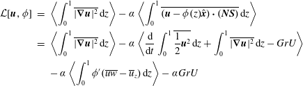 $$\begin{eqnarray}\displaystyle {\mathcal{L}}[\boldsymbol{u},\unicode[STIX]{x1D719}] & = & \displaystyle \left\langle \int _{0}^{1}\overline{|\unicode[STIX]{x1D735}\boldsymbol{u}|^{2}}\,\text{d}z\right\rangle -\unicode[STIX]{x1D6FC}\left\langle \int _{0}^{1}\overline{(\boldsymbol{u}-\unicode[STIX]{x1D719}(z)\hat{\boldsymbol{x}})\boldsymbol{\cdot }(\boldsymbol{N}\boldsymbol{S})}\,\text{d}z\right\rangle \nonumber\\ \displaystyle & = & \displaystyle \left\langle \int _{0}^{1}\overline{|\unicode[STIX]{x1D735}\boldsymbol{u}|^{2}}\,\text{d}z\right\rangle -\unicode[STIX]{x1D6FC}\left\langle \frac{\text{d}}{\text{d}t}\int _{0}^{1}\overline{\frac{1}{2}\boldsymbol{u}^{2}}\,\text{d}z+\int _{0}^{1}\overline{|\unicode[STIX]{x1D735}\boldsymbol{u}|^{2}}\,\text{d}z-GrU\right\rangle \nonumber\\ \displaystyle & & \displaystyle -\,\unicode[STIX]{x1D6FC}\left\langle \int _{0}^{1}\unicode[STIX]{x1D719}^{\prime }(\overline{uw}-\overline{u}_{z})\,\text{d}z\right\rangle -\unicode[STIX]{x1D6FC}GrU\end{eqnarray}$$
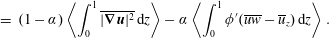 $$\begin{eqnarray}\displaystyle & = & \displaystyle (1-\unicode[STIX]{x1D6FC})\left\langle \int _{0}^{1}\overline{|\unicode[STIX]{x1D735}\boldsymbol{u}|^{2}}\,\text{d}z\right\rangle -\unicode[STIX]{x1D6FC}\left\langle \int _{0}^{1}\unicode[STIX]{x1D719}^{\prime }(\overline{uw}-\overline{u}_{z})\,\text{d}z\right\rangle .\end{eqnarray}$$
At this point, the Euler–Lagrange equations
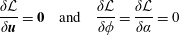 $$\begin{eqnarray}\frac{\unicode[STIX]{x1D6FF}{\mathcal{L}}}{\unicode[STIX]{x1D6FF}\boldsymbol{u}}=\mathbf{0}\quad \text{and}\quad \frac{\unicode[STIX]{x1D6FF}{\mathcal{L}}}{\unicode[STIX]{x1D6FF}\unicode[STIX]{x1D719}}=\frac{\unicode[STIX]{x1D6FF}{\mathcal{L}}}{\unicode[STIX]{x1D6FF}\unicode[STIX]{x1D6FC}}=0\end{eqnarray}$$
contain the background method bound as a solution but there is no means to identify it as such (i.e. appreciate that the associated value of ${\mathcal{L}}$
is a bound on the dissipation rate). Instead, the Otto–Seis approach appears to be to select a simplifying value of
${\mathcal{L}}$
is a bound on the dissipation rate). Instead, the Otto–Seis approach appears to be to select a simplifying value of $\unicode[STIX]{x1D6FC}=1$
so that the right-hand side reduces to
$\unicode[STIX]{x1D6FC}=1$
so that the right-hand side reduces to
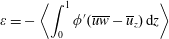 $$\begin{eqnarray}\unicode[STIX]{x1D700}=-\left\langle \int _{0}^{1}\unicode[STIX]{x1D719}^{\prime }(\overline{uw}-\overline{u}_{z})\,\text{d}z\right\rangle\end{eqnarray}$$
and then to choose a simple trial function
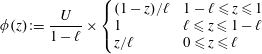 $$\begin{eqnarray}\unicode[STIX]{x1D719}(z):=\frac{U}{1-\ell }\times \left\{\begin{array}{@{}ll@{}}(1-z)/\ell & 1-\ell \leqslant z\leqslant 1\\ 1 & \ell \leqslant z\leqslant 1-\ell \\ z/\ell & 0\leqslant z\leqslant \ell \end{array}\right.\end{eqnarray}$$
(designed so that $\int _{0}^{1}\unicode[STIX]{x1D719}\,\text{d}z=U$
with boundary layers of size
$\int _{0}^{1}\unicode[STIX]{x1D719}\,\text{d}z=U$
with boundary layers of size $\ell$
). This converts (2.12) into
$\ell$
). This converts (2.12) into
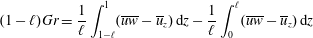 $$\begin{eqnarray}(1-\ell )Gr=\frac{1}{\ell }\int _{1-\ell }^{1}(\overline{uw}-\overline{u}_{z})\,\text{d}z-\frac{1}{\ell }\int _{0}^{\ell }(\overline{uw}-\overline{u}_{z})\,\text{d}z\end{eqnarray}$$
(after using $\unicode[STIX]{x1D700}=UGr$
) which is (4.10) in Seis (Reference Seis2015) and then the strategy is to bound the terms on the right-hand side using powers of
$\unicode[STIX]{x1D700}=UGr$
) which is (4.10) in Seis (Reference Seis2015) and then the strategy is to bound the terms on the right-hand side using powers of $\unicode[STIX]{x1D700}$
. The fundamental observation is that the derivative of the background field is what appears in the Otto–Seis ‘boundary layer’ method (Chernyshenko Reference Chernyshenko2017).
$\unicode[STIX]{x1D700}$
. The fundamental observation is that the derivative of the background field is what appears in the Otto–Seis ‘boundary layer’ method (Chernyshenko Reference Chernyshenko2017).
2.3 Background field for the rough problem
In the rough channel flow problem, the background (vector) field corresponding to the ‘boundary layer’ method as applied in Kerswell (Reference Kerswell2016) is $\unicode[STIX]{x1D719}(\unicode[STIX]{x1D706})\boldsymbol{a}$
(generalised from
$\unicode[STIX]{x1D719}(\unicode[STIX]{x1D706})\boldsymbol{a}$
(generalised from $\unicode[STIX]{x1D719}(z)\hat{\boldsymbol{x}}$
in the smooth-walled problem) where
$\unicode[STIX]{x1D719}(z)\hat{\boldsymbol{x}}$
in the smooth-walled problem) where
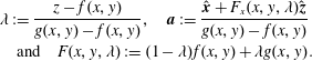 $$\begin{eqnarray}\displaystyle & & \displaystyle \unicode[STIX]{x1D706}:=\frac{z-f(x,y)}{g(x,y)-f(x,y)},\quad \boldsymbol{a}:=\frac{\hat{\boldsymbol{x}}+F_{x}(x,y,\unicode[STIX]{x1D706})\hat{\boldsymbol{z}}}{g(x,y)-f(x,y)}\nonumber\\ \displaystyle & & \displaystyle \quad \text{and}\quad F(x,y,\unicode[STIX]{x1D706}):=(1-\unicode[STIX]{x1D706})f(x,y)+\unicode[STIX]{x1D706}g(x,y).\nonumber\end{eqnarray}$$
For example
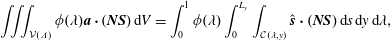 $$\begin{eqnarray}\iiint _{{\mathcal{V}}(\unicode[STIX]{x1D6EC})}\unicode[STIX]{x1D719}(\unicode[STIX]{x1D706})\boldsymbol{a}\boldsymbol{\cdot }(\boldsymbol{N}\boldsymbol{S})\,\text{d}V=\int _{0}^{1}\unicode[STIX]{x1D719}(\unicode[STIX]{x1D706})\int _{0}^{L_{y}}\int _{{\mathcal{C}}(\unicode[STIX]{x1D706},y)}\hat{\boldsymbol{s}}\boldsymbol{\cdot }(\boldsymbol{N}\boldsymbol{S})\,\text{d}s\,\text{d}y\,\text{d}\unicode[STIX]{x1D706},\end{eqnarray}$$
where the right-hand side is (2.6) of Kerswell (Reference Kerswell2016) before integrating with a general weight $\unicode[STIX]{x1D719}(\unicode[STIX]{x1D706})$
over
$\unicode[STIX]{x1D719}(\unicode[STIX]{x1D706})$
over $\unicode[STIX]{x1D706}\in [0,1]$
. Taking
$\unicode[STIX]{x1D706}\in [0,1]$
. Taking $\unicode[STIX]{x1D719}(\unicode[STIX]{x1D706})$
again as the piecewise-linear trial function defined in (2.13) allows the shears associated with it to be controllable. However,
$\unicode[STIX]{x1D719}(\unicode[STIX]{x1D706})$
again as the piecewise-linear trial function defined in (2.13) allows the shears associated with it to be controllable. However, $\boldsymbol{a}$
varies spatially throughout the domain and so the shears associated with the combination do not vanish at some controlled distance from the boundary. This is what prevents the background method working and also has to break the boundary layer method. Unfortunately, this is a known limitation of the background method with no work-around currently on the horizon.
$\boldsymbol{a}$
varies spatially throughout the domain and so the shears associated with the combination do not vanish at some controlled distance from the boundary. This is what prevents the background method working and also has to break the boundary layer method. Unfortunately, this is a known limitation of the background method with no work-around currently on the horizon.
