


1. Introduction
Laser–plasma interactions (LPIs) are usually studied without a background magnetic field, partly because the relevant field strengths are over hundreds of teslas that are difficult to attain, and partly because cyclotron motion significantly complicates physical processes, making the interactions difficult to understand. However, in recent experiments where a seed magnetic field is imposed to enhance thermal and particle confinements in laser-driven inertial fusion experiments (Chang et al. Reference Chang, Fiksel, Hohenberger, Knauer, Betti, Marshall, Meyerhofer, Séguin and Petrasso2011; Hohenberger et al. Reference Hohenberger, Chang, Fiksel, Knauer, Betti, Marshall, Meyerhofer, Séguin and Petrasso2012), understanding magnetised LPIs (MagLPIs) has become necessary. In experiments that are designed using codes that incorporate magnetisation effects on hydrodynamics but not including magnetisation effects on LPIs, the observed hot spot shape is more elongated along the magnetic field than expected (Moody et al. Reference Moody, Pollock, Sio, Strozzi, Ho, Walsh, Kemp, Lahmann, Kucheyev and Kozioziemski2022). Subsequent experiments using manually adjusted laser drive manage to restore the symmetry, suggesting that MagLPIs likely contribute to the discrepancy.
Strong magnetic fields directly affect LPIs in addition to changing plasma conditions. In indirect-drive experiments, external coils apply a seed magnetic field of $B_0\approx 30$ T. This seed field is amplified to the $10^2$
 -T level during the laser drive, when expanding plasmas from the hohlraum wall compresses the magnetic flux near the laser entrance hole (Strozzi et al. Reference Strozzi, Perkins, Marinak, Larson, Koning and Logan2015). Moreover, Biermann-battery fields near the laser spot and flux compression due to the imploding fuel lead to even larger fields at the kilotesla level (Knauer et al. Reference Knauer, Gotchev, Chang, Meyerhofer, Polomarov, Betti, Frenje, Li, Manuel and Petrasso2010; Sio et al. Reference Sio, Moody, Ho, Pollock, Walsh, Lahmann, Strozzi, Kemp, Hsing and Crilly2021). When $B_0\sim 10^2$
 T, electron cyclotron frequency becomes comparable to the frequency of sound waves that mediate Brillouin scattering and cross-beam energy transfer. Moreover, when $B_0\sim 10^3$
 T, the electron cyclotron frequency becomes comparable to the plasma frequency, leading to modifications of the Langmuir wave that mediates Raman scattering and two-plasmon decay. The ability to explain and predict the magnetised version of these commonly encountered long-pulse LPI processes relies on a basic understanding of MagLPIs that we have just begun to acquire.
Although basic facts about unmagnetised LPIs, such as the linear growth rates of Raman and Brillouin scatterings, are well known from decades of theoretical, numerical and experimental studies, simple facts about MagLPIs are poorly understood. The two exceptions are when waves propagate either perpendicular or parallel to the background magnetic field. Perpendicular propagation is particularly relevant for magnetic confinement fusion, where strong radio-frequency pump waves are used for plasma heating and current drive. Using antenna mounted on vacuum chamber walls, the waves are launched nearly perpendicular to the magnetic field. In this geometry, the extraordinary (X) pump can decay to upper-hybrid (UH) and lower-hybrid (LH) waves (Grebogi & Liu Reference Grebogi and Liu1980; Hansen et al. Reference Hansen, Nielsen, Salewski, Stejner and Stober2017), as well as couple with Bernstein waves (Platzman, Wolff & Tzoar Reference Platzman, Wolff and Tzoar1968; Stenflo Reference Stenflo1981). The other special geometry is when waves propagate nearly parallel to the magnetic field, which is particularly relevant for astrophysical-type plasmas, where the pump wave is an Alfvén wave whose frequency is below cyclotron frequencies. In this case, the pump can couple with sound waves and other Alfvén-type waves (Hasegawa & Chen Reference Hasegawa and Chen1976; Wong & Goldstein Reference Wong and Goldstein1986), and the coupling is known also at oblique angles (Viñas & Goldstein Reference Viñas and Goldstein1991). In the context of LPIs, the pump waves are lasers, whose frequencies are typically higher than electron-cyclotron frequency. Most studies of MagLPIs so far are also restricted to special geometries where theories are greatly simplified. In the perpendicular geometry, X-wave pump lasers undergo backscattering (Paknezhad Reference Paknezhad2016; Shi, Qin & Fisch Reference Shi, Qin and Fisch2017a), forward scattering (Hassoon, Salih & Tripathi Reference Hassoon, Salih and Tripathi2009; Babu et al. Reference Babu, Kumar, Jeet, Kumar and Varma2021), second harmonics generation (Jha et al. Reference Jha, Mishra, Raj and Upadhyay2007) and terahertz radiation generation (Varshney et al. Reference Varshney, Sajal, Baliyan, Sharma, Chauhan and Kumar2015). In the parallel geometry, the electrostatic waves are unmagnetised but the right-handed (R) and left-handed (L) circularly polarised electromagnetic waves become non-degenerate, changing the coupling for Raman- and Brillouin-type scatterings (Sjölund & Stenflo Reference Sjölund and Stenflo1967; Laham, Al Nasser & Khateeb Reference Laham, Al Nasser and Khateeb1998). In more general geometry, where waves propagate at oblique angles with respect to the magnetic field, cyclotron motion makes theoretical analysis significantly more complicated. Although theories exist (Larsson & Stenflo Reference Larsson and Stenflo1973; Liu & Tripathi Reference Liu and Tripathi1986; Stenflo Reference Stenflo1994; Brodin & Stenflo Reference Brodin and Stenflo2012), the coupling coefficients are given by cumbersome formulae that are general but rarely evaluated. Physical understanding of underlying processes are largely lacking until recently when more convenient formulae are obtained and evaluated (Shi, Qin & Fisch Reference Shi, Qin and Fisch2017b; Shi Reference Shi2019), leading to pictures of MagLPIs that are both intuitive and quantitative (Shi, Qin & Fisch Reference Shi, Qin and Fisch2018, Reference Shi, Qin and Fisch2021). However, it remains unclear how accurate these formulae are and to what extent they are applicable. Because lasers propagate at oblique angles in inertial fusion experiments, it is especially important to known whether the predicted couplings are correct beyond special angles.
To benchmark analytical formulae, kinetic simulations have been used but systematic comparisons are difficult. When waves propagate perpendicular (Boyd & Rankin Reference Boyd and Rankin1985; Jia et al. Reference Jia, Shi, Qin and Fisch2017) or parallel (Li et al. Reference Li, Zuo, Su and Yang2020, Reference Li, Wu, Zuo, Zeng, Wang, Wang, Mu, Hu and Su2021) to the magnetic field, qualitative agreements between theories and simulations have been found. Moreover, at oblique angles, it is observed that even in regimes where kinetic effects are expected to be important, coupling coefficients predicted by warm-fluid theory are indicative of kinetic simulation results (Edwards et al. Reference Edwards, Shi, Mikhailova and Fisch2019; Manzo, Edwards & Shi Reference Manzo, Edwards and Shi2022). However, systematic comparisons between theory and simulations of MagLPIs have not been made, which is the goal of this paper. Making the comparisons rigorous is difficult for three reasons. First, nonlinear coupling leads to wave growth, but the effect of growth is mixed with damping in kinetic simulations. In the absence of collision, magnetised plasma waves are still damped collisionlessly, whose rate is difficult to calculate because cyclotron motion mixes with trapping motion and particle trajectories are chaotic in general. Even in the simple perpendicular geometry, the two limiting cases, where trapping motion dominates cyclotron motion (Sagdeev & Shapiro Reference Sagdeev and Shapiro1973; Dawson et al. Reference Dawson, Decyk, Huff, Jechart, Katsouleas, Leboeuf, Lembege, Martinez, Ohsawa and Ratliff1983) or vice versa (Karney Reference Karney1978, Reference Karney1979), have drastically different behaviour, and the intermediate regimes are far less understood. As a larger damping can offset a larger growth, their effects need to be separated before coupling coefficients can be constrained. Second, the coupling coefficients derived in theories are specific for eigenmodes but launching eigenmodes in kinetic simulations is not straightforward when waves propagate at oblique angles. In previous simulations, the pump laser is launched with simple linear or circular polarisations from the vacuum region. Upon entering the magnetised plasma, which is a birefringent medium, the laser excites both eigenmodes, which are elliptically polarised at oblique angles. Since nonlinear couplings are different depending on the laser polarisation (Shi & Fisch Reference Shi and Fisch2019), exciting multiple modes does not allow a clean comparison. Finally, additional processes can occur in kinetic simulations, making it difficult to isolate the process of interest. For example, the pump laser can undergo spontaneous scattering into other modes. This problem is particularly severe in particle-in-cell (PIC) simulations, where Monte Carlo sampling noise causes unphysically large spontaneous scattering. As another problem, collisionless damping causes the distribution function to evolve on a time scale that is often comparable to wave growth, which is an issue for both PIC and Vlasov simulations. As coupling coefficients depend on the distribution function, its time evolution complicates the comparison between theories and simulations.
In this paper, one dimensional PIC simulations are used to benchmark coupling coefficients predicted by warm-fluid theory, and excellent agreements between simulations and theory are achieved using a protocol that enables quantitative comparisons. First, to distinguish effects of damping from growth, analytical solutions of the linearised three-wave equation are derived in § 2 and are used to fit simulations data. Building up solutions from initial value problem to boundary value problem, the transient-time spatial profiles in the backscattering problem, where a seed laser is amplified by a counter-propagating pump laser, allows damping and growth rates to be constrained separately. Second, to make numerical results directly comparable to theory, calibration steps are performed for PIC simulations, which are described in § 3. To ensure that a single eigenmode is excited, the pump and seed laser polarisations are calibrated. To account for laser reflections from plasma–vacuum boundaries, laser transmissions are calibrated. To separate pump and seed from raw data and extract their envelopes, phase velocities are calibrated. These calibration runs eliminate free parameters during fitting and make stimulated runs well controlled. Third, competing processes are monitored to ensure that only valid data are used for fitting. Simulation parameters are chosen to reduce the effects of spontaneous scattering, and the seed wavelength is scanned to excite leading resonances, which are mediated by the Langmuir-like P wave and the electron-cyclotron-like F wave. In addition, evolution of the distribution function is monitored to select data within a time window where plasma conditions remain constant. Fitting well-controlled simulation data to analytical solutions of the same set-up leads to excellent agreements in § 3.4, where the warm-fluid theory is shown to be valid within a wide parameter range. The protocol has difficulties for weak resonances, primarily due to spontaneous scattering and leakages during pump–seed separation. Potential ways to circumvent the difficulties are discussed in § 4, and further investigations may find that the warm-fluid theory is valid in even wider parameter spaces. Nevertheless, kinetic effects such collisionless damping and Bernstein-like resonances are clearly observed, suggesting the importance of developing and benchmarking kinetic theories of MagLPIs in the future.
2. Analytic solutions of linearised three-wave equations
In the slowly varying amplitude approximation $E=\mathcal {E}\sin \theta$ , where the wave envelope $\mathcal {E}$
 varies slowly compared with the wave phase $\theta =\boldsymbol {k}\boldsymbol {\cdot }\boldsymbol {x}-\omega t +\theta _0$
 , the interaction between three resonant waves, which satisfy $\omega _1=\omega _2+\omega _3$
 and $\boldsymbol {k}_1=\boldsymbol {k}_2 +\boldsymbol {k}_3$
 , is described by the three-wave equations
where $d_t=\partial _t+\boldsymbol {v}\boldsymbol {\cdot }\boldsymbol {\nabla } +\mu$ is the advective derivative at group velocity $\boldsymbol {v}=\partial \omega /\partial \boldsymbol {k}$
 and $\mu$
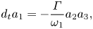
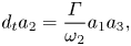
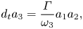
 is a phenomenological damping rate. These equations describe the decay of pump wave $a_1$
 into daughter waves $a_2$
 and $a_3$
 , and the inverse process. The dimensionless $a=e|\mathbf {\mathcal {E}}|u^{1/2}/m_e\omega c$
 is the normalised electric-field amplitude. The normalisation is such that when $a>1$
 , the quiver velocity of electrons, whose charge is $-e$
 and mass is $m_e$
 , becomes comparable to the speed of light $c$
 . The normalisation also involves the wave-energy coefficient $u=\frac {1}{2}\boldsymbol {e}^{\dagger} \it{\boldsymbol{\mathsf{H}}} \boldsymbol {e}$
 , where $\it{\boldsymbol{\mathsf{H}}}$
 is the Hamiltonian of linear waves and $\boldsymbol {e}$
 is the unit polarisation vector, such that the cycle-averaged energy of the wave is $\frac {1}{2}\epsilon _0 u\mathbf {\mathcal {E}}^2$
 . The wave-energy coefficient is simply $u=1$
 for unmagnetised electromagnetic waves and cold Langmuir waves. However, for magnetised plasma waves, $u$
 usually differs from unity and can be evaluated using the code by Shi (Reference Shi2022b) for given eigenmodes.
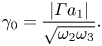
The key parameter in the three-wave equation is the coupling coefficient $\varGamma$ , which has units of frequency squared. In magnetised warm-fluid plasmas, $\varGamma$
 is given by the explicit formula (Shi et al. Reference Shi, Qin and Fisch2017b; Shi Reference Shi2019)

where the summation is over all plasma species, with normalised charge $Z_s=e_s/e$ , mass $M_s=m_s/m_e$
 and plasma frequency $\omega _{ps}^2=e_s^2n_{s0}/\epsilon _0 m_s$
 at equilibrium density $n_{s0}$
 . In the numerator, $\varTheta$
 is due to electromagnetic scattering and is equals to the sum of $\varTheta _{1,\bar {2}\bar {3}}$
 with its five permutations. Explicitly, $\varTheta _{i,jl}=({1}/{\omega _j})(c\boldsymbol {k}_{i}\boldsymbol {\cdot } \boldsymbol {f}_j)(\boldsymbol {e}_{i}\boldsymbol {\cdot }\boldsymbol {f}_l)$
 , where $\boldsymbol {f}=\it{\boldsymbol{\mathsf{F}}} \boldsymbol {e}$
 and $\it{\boldsymbol{\mathsf{F}}}$
 is related to the linear susceptibility by $\it{\boldsymbol{\chi}} =-\omega _p^2 \it{\boldsymbol{\mathsf{F}}} /\omega ^2$
 , which reduces to $\it{\boldsymbol{\mathsf{F}}}=\it{\boldsymbol{\mathsf{I}}}$
 for unmagnetised cold plasmas. The notation $\bar {i}$
 in subscripts means complex conjugation for $\boldsymbol {e}_i$
 and $\boldsymbol {f}_i$
 with negations for the wave 4-momentum $(\omega _i, \boldsymbol {k}_i)$
 . Finally, the $\varPhi^s$
 term in (2.2) is due to warm-fluid nonlinearities, which is typically smaller than $\varTheta^s$
 by a factor of $v_{Ts}^2/c^2$
 , where $v_{Ts}$
 is thermal speed. The coupling coefficient is evaluable using the code from Shi (Reference Shi2022b) once plasma conditions and the three resonant waves are specified.
To benchmark the value of magnetised three-wave coupling coefficient $\varGamma$ using numerical simulations, this paper considers a linearised and one-dimensional problem whereby the three-wave equations are simplified. First, the pump wave is launched with an amplitude that is much larger than the daughter waves, in which case $a_1$
 remains approximately a constant. Second, simulations in one spatial dimension are used, meaning that $\boldsymbol {k}\parallel \hat {\boldsymbol {x}}$
 and the wave envelopes only vary along the $x$
 direction. Note that the group velocity $\boldsymbol {v}$
 can have components in other directions, but $\boldsymbol {v}\boldsymbol {\cdot }\boldsymbol {\nabla }$
 only picks up its $x$
 component $v$
 . With these simplifications, (2.1) becomes a coupled-mode equation $\it{\boldsymbol{\mathsf{L}}} \boldsymbol {\alpha }=\boldsymbol {0}$
 where
where
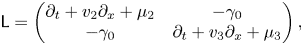
and $\boldsymbol {\alpha }=(\alpha _2, \alpha _3)^\mathrm {T}$ is a column vector. Here, $\alpha =\sqrt {\omega }a$
 is rescaled such that the off-diagonal elements are the same $\gamma _0$
 . As only $\gamma _0^2$
 is of physical significance, we can pick the positive sign so that the bare growth rate of daughter waves is
Without loss of generality, we can always choose to label the daughter waves such that $|v_2|\ge |v_3|$ . Moreover, we can always choose a coordinate such that $v_2\ge 0$
 . With these choices, $\Delta v = v_2-v_3\ge 0$
 is non-negative. Solutions to $\it{\boldsymbol{\mathsf{L}}} \boldsymbol {\alpha }=\boldsymbol {0}$
 are different in forward-scattering ($v_3>0$
 ) and backscattering ($v_3<0$
 ) cases.
As the equations are linear, they admit exponential solutions that are simple to write down analytically but difficult to set up numerically. The exponential solutions are of the form $\alpha _2\propto \alpha _3\propto \exp (\gamma t + \kappa x)$ where the temporal and spatial growth rates satisfy

This constraint defines a hyperbola in the $(\kappa, \gamma )$ plane. One special case is $\kappa =0$
 , where the wave envelopes are uniform in space. The two roots are $\gamma _\pm =-\bar {\mu }\pm \varOmega$
 , where $\bar {\mu }=\frac {1}{2}(\mu _2+\mu _3)$
 , $\varOmega =\sqrt {\gamma _0^2 + ({\Delta \mu }/{2})^2}$
 and $\Delta \mu =\mu _2-\mu _3$
 . When $\gamma _0<\gamma _c$
 , both roots are negative and correspond to damping. On the other hand, when $\gamma _0>\gamma _c$
 , one root becomes positive, giving rise to parametric instability whose threshold is

The other special case is $\gamma =0$ , where the wave envelopes are stationary in time. Assuming $v_2v_3\ne 0$
 , then for forward scattering $v_2v_3>0$
 , the envelopes decay in space unless $\gamma _0>\gamma _c$
 , similar to the previous case. However, the backscattering case $v_2v_3<0$
 is very different: purely growing or decaying solution no longer exists when $\gamma _0$
 exceeds the absolute instability threshold

When $\gamma _0>\gamma _a$ , the two roots of $\kappa$
 acquire imaginary parts, which means that stationary exponential solutions become oscillatory in space. The significance of $\gamma _a$
 will become apparent in (2.25) when we discuss the backscattering problem. To extract growth rates from kinetic simulations, which are usually designed to solve initial boundary value problems, one approach is to choose an initial condition that corresponds to a uniform $\boldsymbol{\alpha}$
 and watch it grow in time. However, the effect of growth is mixed with damping, whose rate is unknown when waves propagate at oblique angles with the magnetic field. An alternative approach is to run simulations until the system reaches steady state. However, the plasma distribution functions also evolve during the process, sometimes quite substantially (Manzo et al. Reference Manzo, Edwards and Shi2022), so the growth and damping are not only mixed but are also not constants. To overcome these difficulties, kinetic simulations are fitted using more general solutions of $\it{\boldsymbol{\mathsf{L}}} \boldsymbol {\alpha }=\boldsymbol {0}$
 by solving initial boundary value problems, whose solutions are known (Bobroff & Haus Reference Bobroff and Haus1967; Hinkel, Williams & Berger Reference Hinkel, Williams and Berger1994; Mounaix & Pesme Reference Mounaix and Pesme1994) but are rederived in the following for clarity. The spatial variations of $\boldsymbol{\alpha}$
 allow the effects of growth and damping to be distinguished, and the transient-time response before plasma conditions evolve allows the growth and damping rates to be treated as constants.
2.1. Initial value problem
In the initial value problem, the spatial domain is infinite, and the wave envelopes evolve in time from their initial conditions
where $\boldsymbol {A}=(A_2, A_3)^\mathrm {T}$ . In the degenerate case $v_2=v_3=v$
 , after transforming to the comoving frame $x'=x-vt$
 and $t'=t$
 where $\partial _t+v\partial _x=\partial _{t'}$
 , the equations become ordinary differential equations (ODEs) in $t'$
 . The eigenvalues $\gamma _\pm =-\bar {\mu }\pm \varOmega$
 of the linear ODEs are the $\kappa =0$
 roots of (2.5), and the general solutions are of the form $\alpha (x',t')=A_+(x')\exp ({\gamma _+t'}) + A_-(x')\exp ({\gamma _-t'})$
 . The coefficients $A_\pm$
 are determined by matching initial conditions, which give the solution

The $\Delta v=0$ solution exhibits two features that are more general: a diagonal damping term and off-diagonal coupling terms that vanish when $\gamma _0=0$
 . The rest of this paper focuses on the non-degenerate case $\Delta v>0$
 , because in LPIs $v_2$
 is close to the speed of light whereas $v_3$
 is on the scale of thermal velocities, which are much slower.
In the non-degenerate case $\Delta v> 0$ , because the equations are linear, they can be solved using Fourier transform $\mathcal {F}[p](k)=\int _{-\infty }^{+\infty } {{\rm d}x}\,p(x) \exp ({-{\rm i}kx})=\hat {p}(k)$
 . In momentum space, the equation becomes $\partial _t\hat {\boldsymbol {\alpha }}={\boldsymbol{\mathsf{K}}} \hat {\boldsymbol {\alpha }}$
 where
where
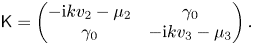
As the matrix is time independent, the solution is $\hat {\boldsymbol {\alpha }}(t)=\exp (t {\boldsymbol{\mathsf{K}}} ) \hat {\boldsymbol {A}}$ . The matrix exponential can be computed by diagonalising $\it{\boldsymbol{\mathsf{K}}}$
 whose eigenvalues are $\lambda _\pm =-{\rm i}k\bar {v}-\bar {\mu }\pm \sqrt {\gamma _0^2-\omega ^2}$
 , where $\bar {v}=\frac {1}{2}(v_2+v_3)$
 and $\omega =\frac {1}{2}(k\Delta v-{\rm i}\Delta \mu )$
 . Finding eigenvectors of $\lambda _\pm$
 and diagonalising $\it{\boldsymbol{\mathsf{K}}}$
 , the solution map $\hat {\it{\boldsymbol{\varPhi }}}(k,t)=\exp (t \it{\boldsymbol{\mathsf{K}}} )$
 can be written as

where $\hat {G}(k,t) = \sinh (t\sqrt {\gamma _0^2-\omega ^2})/\sqrt {\gamma _0^2-\omega ^2}$ . The solution map $\hat {\it{\boldsymbol{\varPhi }}}(k,t)$
 satisfies matrix equation $\partial _t \hat {\it{\boldsymbol{\varPhi }}}(k,t)={\boldsymbol{\mathsf{K}}} \hat {{\boldsymbol{\varPhi }}}(k,t)$
 and initial condition $\hat {\it{\boldsymbol{\varPhi }}}(k,t=0)=\it{\boldsymbol{\mathsf{I}}}$
 , where $\it{\boldsymbol{\mathsf{I}}}$
 is the two-dimensional identity matrix. Note that the behaviour of $\hat {G}$
 is regular when $\omega (k)\rightarrow \pm \gamma _0$
 . We can choose the branch cut for the square roots to lie between these two points. As $\sinh$
 is an odd function, $\hat {G}$
 is, in fact, analytic in the complex $k$
 plane.
To find the solution in $x$ space, take inverse Fourier transform $\mathcal {F}^{-1}[\hat {p}](x) =\int _{-\infty }^{+\infty } ({{\rm d} k}/{2{\rm \pi} }) \hat {p}(k) \exp({\rm i}kx) =p(x)$
 . As $\omega$
 depends on $k$
 , it is convenient to change the integration variable to $k'=2\omega /\Delta v$
 , which gives $k=k'+{\rm i}\Delta \mu /\Delta v$
 . Moreover, it is convenient to change the reference frame to


which travels at the average velocity of the two waves. Note that $z-\tau =x-v_2t$ and $z+\tau =x-v_3t$
 . The phase factor simplifies as $\exp [{\rm i}kx-({\rm i}k\bar {v}+\bar {\mu })t]=\rho \exp ({{\rm i}k'z})$
 where
where
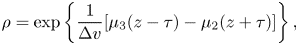
which is a damping factor independent of $k'$ . When taking inverse Fourier transform of (2.11), all matrix elements can be expressed in terms of

where $m=2\gamma _0/\Delta v$ , $I_0$
 is modified Bessel function and $\varTheta$
 is Heaviside step function. The shift by $\epsilon = \Delta \mu /\Delta v$
 is insignificant because the integrand is analytic. The above integral is calculated in Appendix A. The solution map $\it{\boldsymbol{\varPhi }}$
 in configuration space is
The derivatives are evaluated using $I'_0(\xi )=I_1(\xi )$ and $\varTheta '(\xi )=\delta (\xi )$
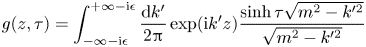
 , and an explicit formula is given by (A7). The function $g$
 satisfies the imaginary-mass Klein–Gordon equation $(\partial _\tau ^2-\partial _z^2-m^2)g(z,\tau )=0$
 , as shown in (A5). Consequently, the solution map satisfies $\it{\boldsymbol{\mathsf{L}}} \it{\boldsymbol{\varPhi}} (x,t)=\it{\boldsymbol{\mathsf{0}}}$
 following (A6). The step function $\varTheta$
 enforces the causality that information outside the light cone $\tau ^2-z^2=(v_2t-x)(x-v_3t)$
 does not affect solutions.
Finally, to invert $\hat {\boldsymbol {\alpha }}=\hat {\it{\boldsymbol{\varPhi }}}\hat {\boldsymbol {A}}$ , compute inverse Fourier transform of products, which are given by convolutions $\mathcal {F}^{-1}[\hat {p}\hat {q}](x)=\int _{-\infty }^{+\infty } {{\rm d}x}'\, p(x')q(x-x')$
 . As the phase factor is simpler in $k'=k-{\rm i}\Delta \mu /\Delta v$
 , in addition to the change of variables in (2.12), it is convenient to define $\hat {\boldsymbol {B}}(k')= \hat {\boldsymbol {A}}(k)$
 , which means that $\boldsymbol {B}(x) = \exp (x\Delta \mu /\Delta v)\boldsymbol {A}(x)$
 . With $\boldsymbol {\alpha }=\rho \boldsymbol {\beta }$
 , where $\rho$
 is given by (2.13), the solution can be written as


where $\xi '=m\sqrt {\tau ^2-z'^2}$ . An explicit expression of $\boldsymbol {\alpha }$
 in $(x,t)$
 coordinate is given later in (2.19). It is straightforward to check that the expression satisfies the differential equation and the initial conditions. When $\boldsymbol {B}$
 only involves $\delta$
 or step functions, the integrals can be readily evaluated. However, for general initial conditions, closed-form analytical expressions may not exist, so the integrals are evaluated numerically. Compared with numerical integration of the differential equations, which advances initial conditions step by step, the integral solution allows fast forwarding, which directly gives the solution at desired final time. Note that by rescaling $z'=\tau \zeta$
 , the numerical integration is always within the range $\zeta \in [-1,1]$
 , so the cost of evaluating the integral does not increase with time for smooth initial conditions.
2.2. Initial boundary value problem
Compared with the initial value problem, the boundary value problem is easier to set up in kinetic simulations. In the initial value problem, the distribution functions need to be specified meticulously in both the configuration space and the velocity space in order to ensure that only the desired eigenmodes are excited. In comparison, in a boundary value problem, only electromagnetic fields at the boundary need to be specified. Using wave frequencies and polarisations to select excited waves, the desired eigenmodes then propagate into the initially Maxwellian plasma where interactions occur. With a single boundary at $x=0$ , the initial boundary value problem is specified by conditions


where $\boldsymbol {h}=(h_2,h_3)^\mathrm {T}$ . In the forward-scattering case $v_2>v_3>0$
 , these conditions can be specified separately. However, in the backscattering case $v_2>0>v_3$
 , in order for the problem to be well-posed, only two conditions can be specified independently.
As the equation $\it{\boldsymbol{\mathsf{L}}} \boldsymbol {\alpha }=\boldsymbol {0}$ is linear, the initial boundary value problem can be solved using Laplace transform $\mathcal {L}[p](k)=\int _{0}^{+\infty } {{\rm d}x}\,p(x) \exp ({-{\rm i}kx}) =\tilde {p}(k)$
 . Using the property of Laplace transform that $\tilde {p}'(k)={\rm i}k\tilde {p}(k)-p(0)$
 , the equation becomes $\partial _t\tilde {\boldsymbol {\alpha }}={\boldsymbol{\mathsf{K}}} \tilde {\boldsymbol {\alpha }}+\it{\boldsymbol {H}}$
 , where $\it{\boldsymbol{\mathsf{K}}}$
 is given by (2.10) and $\it{\boldsymbol {H}}=(v_2h_2,v_3h_3)^\mathrm {T}$
 . Using the Duhamel's principle, the inhomogeneous ODE is solved by $\tilde {\boldsymbol {\alpha }}(t)=\hat {\it{\boldsymbol{\varPhi }}}(t)\tilde {\boldsymbol {A}}+ \int _0^t {\rm d} t' \,\hat {\it{\boldsymbol{\varPhi }}} (t-t')\boldsymbol {H}(t')$
 , where $\hat {\boldsymbol{\varPhi }}$
 is given by (2.11). To find the solution in configuration space, take inverse Laplace transform $\mathcal {L}^{-1}[\hat {p}\tilde {q}](x)=\int _\mathcal {C} ({{\rm d} k}/{2{\rm \pi} }) \mathcal {F}[p](k)\mathcal {L}[q](k) \exp({\rm i}kx)=\int _0^{+\infty } {{\rm d}x}' p(x-x')q(x')$
 , where the contour $\mathcal {C}$
 runs below all poles. The solution is

where $\it{\boldsymbol{\varPhi}}$ is given by (2.15). Using $\it{\boldsymbol{\mathsf{L}}} \it{\boldsymbol{\varPhi}} =\it{\boldsymbol{\mathsf{0}}}$
 , the expression clearly satisfies $\it{\boldsymbol{\mathsf{L}}} \boldsymbol {\alpha }=\boldsymbol {0}$
 . Moreover, using the explicit expression of $\it{\boldsymbol{\varPhi}}$
 in (A7), it is easy to see that $\it{\boldsymbol{\varPhi}} (x,t=0)=\delta (x) \it{\boldsymbol{\mathsf{I}}}$
 , so the initial conditions are always satisfied. However, the situation for boundary conditions depends on the sign of $v_3$
 , as shown in the following.
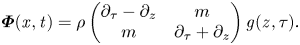
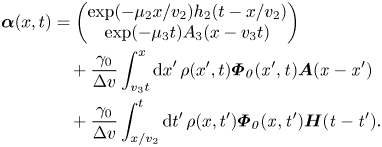
Using the property that $\it{\boldsymbol{\varPhi}}$ is zero outside the light cone, the above integral solution, which is equivalent to $\boldsymbol {\alpha }(x,t)=\int _{-\infty }^x {{\rm d}x}'\,\it{\boldsymbol{\varPhi}} (x',t)\boldsymbol {A}(x-x')+\int _0^t {\rm d} t'\,\it{\boldsymbol{\varPhi}}(x,t')\boldsymbol {H}(t-t')$
 , is simplified in the three regions shown in figure 1. First, ahead of the light cone $x>v_2t$
 , effects of boundary conditions have not arrived, so only the initial conditions contribute. In terms of the rescaled variable $\boldsymbol {\beta }$
 , the solution is given by (2.16), and in terms of the original variables, the solution when $x>v_2t>0$
 is
is

where $\rho$ is the damping factor given by (2.13) and $\it{\boldsymbol{\varPhi}} _0$
 is the kernel within the light cone given in (A7). When $t=0$
 , the solution clearly satisfies the initial conditions. Second, behind the light cone $x< v_3t$
 , which is within the domain only when $v_3>0$
 , effects of the initial conditions have propagated away, so only the boundary conditions contribute. Therefore, when $v_3t>x>0$
 , the solution is

The solution clearly satisfies the boundary conditions at $x=0$ for this forward-scattering case. Finally, inside the light cone, both the initial and boundary conditions contribute, and the solution when $v_3t< x< v_2t$
 is given by
In the forward-scattering case $v_3>0$ , the future light cone is within the domain, so the initial and boundary conditions can be specified independently. However, in the backscattering case $v_3<0$
 , the future light cone is intercepted by the boundary. Intuitively, when information propagates towards left and arrives at the boundary, one cannot arbitrarily set values at the boundary.
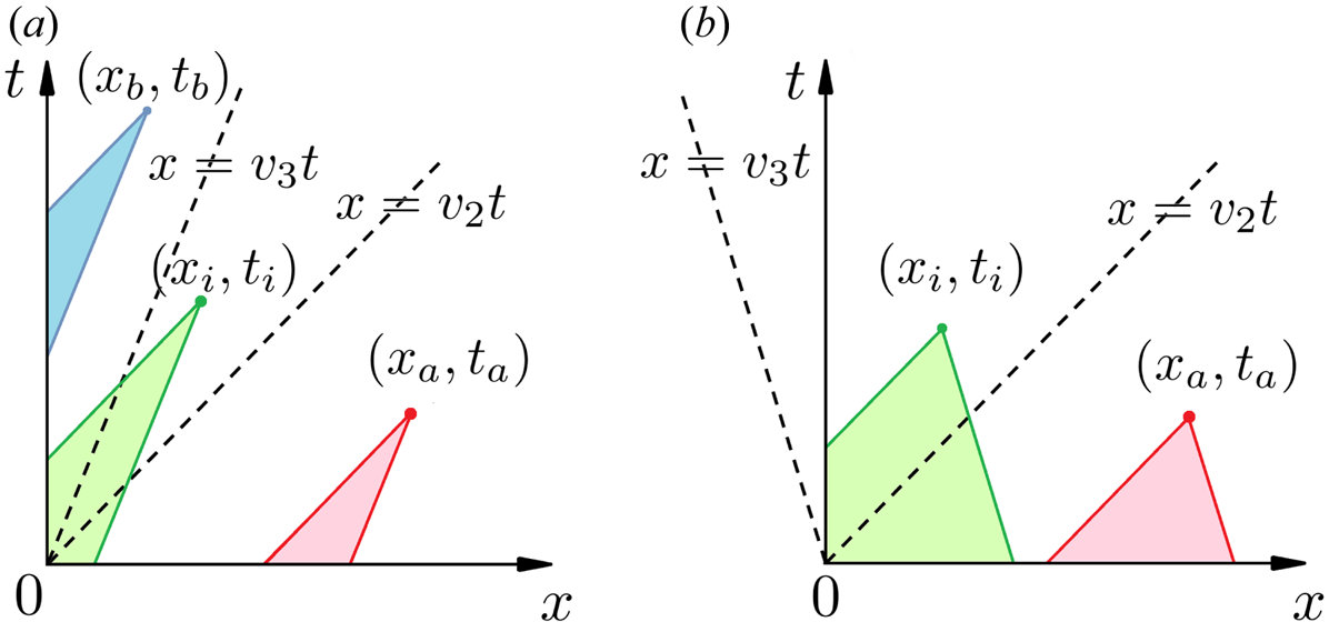
Figure 1. Solutions are determined by initial and boundary conditions within the past light cone. For $(x_a, t_a)$ ahead of $x>v_2t$
 , the light cone (red) only intercepts the $x$
 axis, so the solution is independent of boundary conditions. For $(x_b, t_b)$
 behind $x< v_3t$
 , the light cone (blue) only intercepts the $t$
 axis, so the solution is independent of initial conditions. For $(x_i, t_i)$
 within $v_3t< x< v_2t$
 , the solution depends on both initial and boundary conditions. (a) In the forward-scattering case, initial and boundary conditions can be specified independently. (b) In the backscattering case, initial conditions arrive at the boundary so constraints must be satisfied.
2.3. Backscattering problem
When the initial conditions are zero, as is the case in kinetic simulations, the integral constraints $\boldsymbol {\alpha }(x=0,t>0)=\boldsymbol {h}(t)$ for the backscattering case $v_3<0$
 can be solved explicitly. By setting $x=0$
 and $\boldsymbol {A}=\boldsymbol {0}$
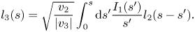
 in (2.21), the constraints can be simplified as $(0, l_3(s))^\mathrm {T}=\int _0^s {\rm d} s'\,\it{\boldsymbol{\varPsi}} _0(s')\boldsymbol {l}(s-s')$
 , where $s=\gamma t$
 is time normalised by $\gamma =2\gamma _0\sqrt {v_2|v_3|}/\Delta v$
 , $\boldsymbol {l}(s)={\rm e}^{\mu t}\boldsymbol{h}(t)$
 is rescaled by damping $\mu =(\mu _3v_2+\mu _2|v_3|)/\Delta v$
 , and
, and

Note that $\mu t=s\gamma _a/\gamma _0$ , where $\gamma _a$
 is the absolute instability threshold given by (2.7). As the constraint is a convolution, it becomes a product after taking Laplace transform, which gives $(0, \tilde {l}_3(\omega ))^\mathrm {T} =\tilde {\it{\boldsymbol{\varPsi}}}_0(\omega )\tilde {\boldsymbol {l}}(\omega )$
 . To compute $\tilde {\it{\boldsymbol{\varPsi}}}_0$
 , use integral representation of modified Bessel function (DLMF 2022, (10.32.2)) that $I_0(s)=({1}/{{\rm \pi} })\int _{-1}^1 {\rm d} t \exp(-st)/\sqrt {1-t^2}$
 and perform the $s$
 integral first, which gives $\tilde {I}_0(\sigma ) = 1/\sqrt {\sigma ^2-1}$
 where $\sigma ={\rm i}\omega$
 . Then, $\tilde {I}_1(\sigma ) = \sigma /\sqrt {\sigma ^2-1}-1$
 because $I_1(s)=I'_0(s)$
 . As $I_n(s)\simeq {\rm e}^s/\sqrt {2{\rm \pi} s}$
 when $s\rightarrow \infty$
 , the Laplace transforms converge only when $\rm{Re}(\sigma )>1$
 . Solving the constraint in frequency domain gives a unique solution
which means that if we specify the boundary condition for $\alpha _2$ , then the boundary condition for $\alpha _3$
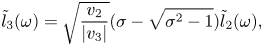
 is completely determined. Taking inverse Laplace transform, whose details are shown in Appendix B, the self-consistent boundary condition is
When the normalised time $s=0$ , the boundary condition $l_3(0)=0$
 is initially quiescent. At later time, $\alpha _3$
 builds up due to wave growth and advection. As shown in Appendix B, we can also express $l_2$
 in terms of $l_3$
 . However, in kinetic simulations, it is much easier to specify the boundary conditions for electromagnetic waves and let the plasma evolve to fulfill the above boundary condition.
Having expressed $h_3$ in terms of $h_2$
 , the solution of $\boldsymbol {\alpha }$
 is a functional of $h_2$
 only. The integrals simplify when $h_2$
 is $\delta$
 or $\varTheta$
 functions. As $\delta$
 functions cannot be resolved numerically, let us focus on the case $h_2(t)=h_0\varTheta (t)$
 , which is used later to set up kinetic simulations. Using (2.24) with $l_2(s)=h_0\exp ({s\gamma _a/\gamma _0}) \varTheta (s)$
 , $h_3(t)=h_0\sqrt {v_2/|v_3|}\int _0^{\gamma t} {\rm d} s' \exp ({-s'\gamma _a/\gamma _0}) I_1(s')/s'$
 . Substituting $\boldsymbol {h}$
 into (2.21), changing integration variable to $\varphi '=\gamma (t'-x/v_2)$
 , and rotating the triangular double integral in a way that leads to (B5) gives


whereas $\boldsymbol {\alpha }(x>v_2t)=\boldsymbol {0}$ ahead of the wave front. In these expressions, $\gamma =2\gamma _0\sqrt {v_2|v_3|}/\Delta v$
 , $\vartheta =\gamma _0x/\sqrt {v_2|v_3|}$
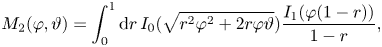
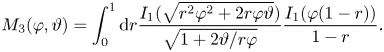
 , $D_2(\varphi, \vartheta ) = \sqrt {1+2\vartheta /\varphi }I_1(\sqrt {\varphi ^2+2\varphi \vartheta })-M_2(\varphi, \vartheta )$
 and $D_3(\varphi, \vartheta ) = I_0(\sqrt {\varphi ^2+2\varphi \vartheta })-M_3(\varphi, \vartheta )$
 , where the kernel functions are
The differential properties of the kernel functions (C3) and (C4) ensures that (2.25) satisfies $\it{\boldsymbol{\mathsf{L}}}\boldsymbol {\alpha }=\boldsymbol {0}$ . Moreover, the special values $D_2(\varphi, 0)=0$
 and $D_3(\varphi, 0)=2I_1(\varphi )/\varphi$
 (C1) and (C2) ensure that the boundary conditions are satisfied. Using these special values, we see $\alpha _3\rightarrow +\infty$
 when $t\rightarrow +\infty$
 at $x=0$
 if $\varsigma =\gamma _a/\gamma _0<1$
 , whereas $\alpha _3\rightarrow h_0\sqrt {v_2/|v_3|}(\varsigma - \sqrt {\varsigma ^2-1})$
 if $\varsigma \ge 1$
 . More generally when $x\ge 0$
 , the solutions approach steady state if and only if $\gamma _0$
 does not exceed the absolute instability threshold. The solutions are of the form $\alpha _2=h_0 \exp ({-\mu _2x/v_2})(1+\Delta _2)$
 and $\alpha _3=h_0\exp ({-\mu _2x/v_2})\Delta _3$
 . Examples of the growth function $\Delta _j$
 are plotted in figures 2 and 3.

Figure 2. The growth function $\Delta _j(x)$ in the step-function backscattering problem for (a) the seed laser and (b) the plasma wave at selected time slices when $v_2=3\times 10^8$
 m s$^{-1}$
 , $\gamma _0=10^{13}$
 rad s$^{-1}$
 and $\mu _2=0$
 . As time increases, $\Delta _j$
 propagates in space and grows in amplitude. The growth is always zero ahead of the wave front $x=v_2t$
 . Moreover, $\Delta _2(0)$
 is always zero due to the boundary condition. In contrast, $\Delta _3(0)$
 builds up from zero as time increases. Compared with the dampingless case (red lines), having an appreciable $\mu _3$
 (blue lines) reduces the growth. Compared with the $v_3=0$
 case (blue lines), having a small $v_3$
 (cyan circles) slightly affects the solutions at early time. At later time, the discrepancies build up because $\gamma _0\approx 1.3\gamma _a$
 exceeds the absolute instability threshold.

Figure 3. The growth function $\Delta _j(t)$ in the step-function backscattering problem for (a) the seed laser and (b) the plasma wave at $x=20\,\mathrm {\mu }\rm{m}$
 when $v_2=3\times 10^8$
 m s$^{-1}$
 , $\mu _3=5\times 10^{12}$
 rad s$^{-1}$
 and ${\mu _2=0}$
 . When $v_3=-v_2/10$
 (symbols), the absolute instability threshold is $\gamma _a\approx 7.8\times 10^{12}$
 rad s$^{-1}$
 . When $\gamma _0=7\times 10^{12}$
 rad s$^{-1}$
 (cyan) is below the threshold, the growth approaches steady state. In contrast, when $\gamma _0=10^{13}$
 rad s$^{-1}$
 (magenta) exceeds the threshold, $\Delta _j$
 continues to increase. When $v_3=0$
 (lines), $\gamma _a$
 becomes infinite so the growth always saturates. The case with $\gamma _0=10^{13}$
 rad s$^{-1}$
 (red) has a larger steady-state value than the case with $\gamma _0=7\times 10^{12}$
 rad s$^{-1}$
 (blue). The effects of a small but finite $v_3$
 only become significant at later time.
The integral solutions for the step-function problem are greatly simplified when $v_3\rightarrow 0$ , which is a good approximation for LPIs where $v_2\gg |v_3|$
 . Inside the domain, $\vartheta \rightarrow \infty$
 but $\gamma \rightarrow 0$
 , whereas $\gamma \vartheta =2\gamma _0^2x/v_2$
 is finite. As the integrands in (2.26) approach zero when $\varphi \rightarrow 0$
 at fixed $\varphi \vartheta$
 , both $M_2$
 and $M_3$
 become zero. Then, $D_2\rightarrow \xi I_1(\xi )/\varphi$
 and $D_3\rightarrow I_0(\xi )$
 , where $\xi =\sqrt {2\varphi \vartheta }$
 . Writing integrals in (2.25) in terms of $\xi$
 gives
gives

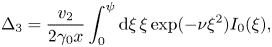
where $\psi =2\gamma _0\sqrt {(t-x/v_2)x/v_2}$ and $\nu =\mu _3v_2/4x\gamma _0^2$
 . Observe that $\psi =\sqrt {\mu _3t_r/\nu }$
 where $t_r=t-x/v_2$
 is the retarded time since the wave front passes, and $1/4\nu$
 is the spatial gain exponent in steady state when $\mu _2=0$
 . After integration by parts, $\Delta _3=(\gamma _0/\mu _3)[1-I_0(\psi ) \exp ({-\nu \psi ^2})+\Delta _2]$
 . It is straightforward to verify that (2.27) solves $\it{\boldsymbol{\mathsf{L}}} \boldsymbol {\alpha }=\boldsymbol {0}$
 when $v_3=0$
 . When $t\rightarrow +\infty$
 , the solutions approach steady states, which are always finite because $\gamma _a\rightarrow \infty$
 . Using Gaussian integrals of modified Bessel function (DLMF 2022, (10.43.24)), $\Delta _2=\exp (1/4\nu )-1-\mathcal {R}$
 . As shown in Appendix C, the residual $\mathcal {R}=\int _\psi ^{+\infty }{\rm d}\xi \exp ({-\nu \xi ^2})I_1(\xi )$
 decays as $\exp ({-\mu _3t_r})$
 when $\mu _3t_r\gg \max (1,\gamma _0^2x/\mu _3v_2)$
 . The steady states $\alpha _2(x,+\infty )=(\mu _3/\gamma _0)\alpha _3(x,+\infty )=h_0 \,{\rm e}^{\kappa x}$
 , where $\kappa =(\gamma _0^2/\mu _3-\mu _2)/v_2$
 , are consistent with linear stability analysis of (2.5). The formulae in (2.27) are further simplified in two limiting cases. (1) When $\nu \rightarrow +\infty$
 , namely, when spatial gain is negligible, integrals are dominated by values near $\xi \simeq 0$
 . The growths $\Delta _2\simeq (\gamma _0^2x/\mu _3v_2)(1-\exp ({-\mu _3t_r}))\rightarrow 0$
 and $\Delta _3\simeq (\gamma _0/\mu _3)(1-\exp ({-\mu _3t_r}))$
 . (2) When $\mu _3\rightarrow 0$
 , the Gaussian weight becomes unity. Using properties of modified Bessel function (DLMF 2022, (10.43.1)), the integrals are evaluated to $\Delta _2=I_0(\psi )-1$
 and $\Delta _3=(v_2/2\gamma _0 x)\psi I_1(\psi )$
 . When $\psi \simeq 0$
 , which occurs near the boundary or the wave front, $\Delta _2\simeq \gamma _0^2t_rx/v_2$
 and $\Delta _3\simeq \gamma _0 t_r$
 grow linearly in time. At given $t$
 , the maximum of $1+\Delta _2$
 is attained at $x=\frac {1}{2}v_2 t$
 , which propagates at half the wave group velocity. The maximum value attained at $\psi =\gamma _0t$
 is $I_0(\gamma _0 t)\simeq {\rm e}^{\gamma _0t}/\sqrt {2{\rm \pi} \gamma _0t}$
 when $t\rightarrow +\infty$
 . Although the exponential growth ${\rm e}^{\gamma _0t}$
 is intuitive, the suppression by $1/\sqrt {2{\rm \pi} \gamma _0t}$
 is perhaps not one would naïvely expect from linear instability analysis.
3. Kinetic simulations of stimulated backscattering
To benchmark the formula for magnetised three-wave coupling coefficients in the backscattering geometry, analytic solutions of the step-function problem are used to fit kinetic simulations in the same set-up, where the simulations are performed using the PIC code EPOCH (Arber et al. Reference Arber, Bennett, Brady, Lawrence-Douglas, Ramsay, Sircombe, Gillies, Evans, Schmitz and Bell2015). For the step-function problem, the initial condition is simply a quiescent Maxwellian plasma, whose density is chosen to be $n_e=n_i=n_0=10^{19}\,\mathrm {cm}^{-3}$ and temperature $T_e=T_i=T_0$
 will be scanned. The two species have the mass ratio $M_i=m_i/m_e=1837$
 of hydrogen plasmas. In the one-dimensional simulation domain, the plasma occupies $x\in [0,L_p]$
 with a constant $n_0$
 and $T_0$
 , and two vacuum gaps each of length $L_v$
 are placed on either side, where $L_p=80\lambda _1$
 , $L_v=10\lambda _1$
 and $\lambda _1=1\,\mathrm {\mu }$
 m is the vacuum pump wavelength. The slowly varying envelope approximation requires that $L_p\gg \lambda _1$
 . A constant magnetic field of strength $B_0$
 is applied in the $x$
 –$z$
–$z$ plane at an angle $\theta _B$
 with respect to the $x$
 axis. The special case $B_0=0$
 is unmagnetised, and the special angle $\theta _B=0$
 means wave vectors are parallel to the magnetic field. Both $B_0$
 and $\theta _B$
 will be scanned.
To achieve a constant pump amplitude, the laser is launched from the right domain boundary and ramped up from zero using a $\tanh$ profile whose temporal width equals to the laser period. The smooth ramp reduces oscillations due to numerical artefacts yet is fast enough to be viewed as a step function for the slowly varying envelope. After propagating across the vacuum gap, most pump energy transmits into the plasma, and a small fraction is reflected from the plasma–vacuum boundary. The reflected pump leaves the domain from its right boundary, and the transmitted pump amplitude is measured from simulation data. Using analytical wave energy coefficient, the pump amplitude is normalised to $a_1$
 , which enters the growth rate $\gamma _0$
 in (2.4). When the pump reaches the plasma–vacuum boundary on the left, most energy exists the plasma, but a small fraction is reflected. As its wave vector is flipped, the reflected pump does not interact with the seed laser resonantly but copropagates with the seed in $+x$
 direction.
The seed laser $\alpha _2$ is launched from the left domain boundary using a similar profile but with a time delay such that its wave front enters the plasma after the pump front has exited. To measure the transmitted seed amplitude into the plasma, a seed-only run is performed to fit the boundary condition $h_0$
 in the step-function problem. After the calibration steps, a stimulated run is performed where both the pump and seed lasers are turned on. The simulation is terminated slightly before the seed front reaches $x=L_p$
 , so that the analytical solution, which is obtained when only the left boundary is present, remains applicable. In addition, both the electron distribution function $f_e(v_x)$
 and the pump wave amplitude $a_1(x)$
 are monitored during the simulations. In many cases, the change of $f_e$
 and $a_1$
 are small. For example, when the three-wave coupling is weak and the propagation angle $\theta _B$
 is small (figure 4a), the distribution function stays close to the initial Maxwellian. In comparison, when the coupling is week but angle is close to $90^\circ$
 (figure 4d), even though $f_e$
 remains largely constant during the interaction, it is broadened from the Maxwellian due to quiver motion in the pump laser, which has an appreciable longitudinal component. The situation is different when the coupling is strong. Regardless of the angle, when a large-amplitude plasma wave is excited, its collisionless damping leads to substantial broadening of $f_e$
 as shown in figures 4(b) and 4(c), which correlates with a significant increase of the plasma energy (figure 4e) and a rapid depletion of the pump laser. The simulation data after the peak of $f_e$
 reduces by $5\,\%$
 or $a_1$
 drops by $1\,\%$
 since interactions began are excluded from fitting, which assumes constant plasma conditions and pump amplitude.
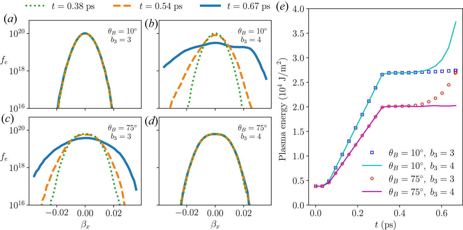
Figure 4. Plasma evolves as pump fills and seed grows. (a) When $\theta _B=10^\circ$ and the coupling is weak, distribution function $f_e(\beta _x)$
 , where $\beta _x=v_x/c$
 , stays near the initial Maxwellian. (b) When $\theta _B=10^\circ$
 but the coupling is strong, $f_e$
 broadens rapidly. At $t=0.38$
 ps (dotted green), $f_e$
 is still close to Maxwellian, but when $t=0.54$
 ps (dashed orange), non-Maxwellian tails develop. By $t=0.67$
 ps (solid blue), a plateau-like feature resembles particle trapping in unmagnetised Landau damping. (c) When $\theta _B=75^\circ$
 and the coupling is strong, $f_e$
 also broadens significantly. In this case, $f_e$
 remains largely symmetric due to mixing effects of gyro motion. (d) When $\theta _B=75^\circ$
 but the coupling is weak, $f_e$
 barely evolves but is no longer Maxwellian due to longitudinal quiver motion in the pump laser. (e) The plasma areal energy density is initially thermal $U_T=3T_0n_0L_p\approx 0.38\times 10^4\,\mathrm {J}\,{\rm m}^{-2}$
 . As the pump fills in, plasma energy increases due to quiver motion. In unmagnetised plasma, $U_Q=\frac {1}{2}m_ec^2a_1^2n_0L_p\approx 2.4\times 10^4\,\mathrm {J}\,{\rm m}^{-2}$
 . However, due to magnetisation, the increase depends on $\theta _B$
 . After the seed enters, energy increases further if plasma waves are strongly excited. In these examples, $B_0=3$
 kT, $T_0=10$
 eV, $I_1=10^{15}\,{\rm W}\,{\rm cm}^{-2}$
 and $I_2=5\times 10^{12}\,{\rm W}\,{\rm cm}^{-2}$
 . In (a,c), the interactions are mediated by F waves whose branch index is $b_3=3$
 , namely, the third highest frequency branch in the warm-fluid dispersion relation. In (b,d), the interactions are mediated by P waves with $b_3=4$
 .
.
The choice of pump and seed laser intensities are constrained by three factors. First, numerical noise of the PIC method gives an upper bound of the pump intensity due to spontaneous scattering. With a finite number of sampling particles, the plasma density fluctuates around $n_0$ , leading to a noise $\delta E_\parallel$
 that can spontaneously scatter the pump laser $a_1$
 . For scatterings mediated by electron modes, the growth rate is typically comparable to the cold Raman backscattering rate $\gamma _R=\frac {1}{2}a_1(\omega _p\omega _1)^{1/2}$
 . The requirement $\gamma _R t_p\lesssim 1$
 that noise does not grow substantially gives an upper bound for the pump intensity, where $t_p\simeq L_p/c$
 is the time it takes for the pump to fill the plasma. As $\gamma _R t_p={\rm \pi} (n_0/n_c)^{1/4}(L_p/\lambda _1) a_1$
 , where $n_c=\epsilon _0m_e\omega ^2/e^2\approx 1.1\times 10^{21}\lambda _{\mathrm {\mu }\mathrm {m}}^{-2}\,\mathrm {cm}^{-3}$
 is the critical density, we need $a_1\ll 10^{-1}$
 for earlier choices of $n_0$
 and $L_p$
 . In terms of laser intensity, because $a_1\simeq 8.6\times 10^{-3} \lambda _{\mathrm {\mu }\mathrm {m}} I_{14}^{1/2}$
 , where $I_{14}$
 is the intensity in units of $10^{14}\,\mathrm {W}\,{\rm cm}^{-2}$
 , we see that the pump intensity cannot far exceed $I_{14}\sim 10^2$
 . Second, PIC noise also imposes a lower bound for the seed intensity. In each cell, the distribution function is sampled with $N$
 super particles. Even though the mean velocity is zero, the standard error of the mean is $\delta v=v_T/\sqrt {N}$
 , where $v_T/c\approx 6.3\times 10^{-2}T_{\mathrm {keV}}^{1/2}$
 is the electron thermal speed. The sampling error leads to a noise current density $\delta j=en_0\delta v$
 , which drives a noise field $\delta E_\perp =\delta j/\epsilon _0\omega$
 at frequency $\omega$
 through Ampère's law. In terms of the relativistic critical field $E_c=m_e\omega c/e\approx 3.2\times 10^{12}\lambda _{\mathrm {\mu }\mathrm {m}}^{-1}\,\mathrm {V}\,{\rm m}^{-1}$
 , the error field at the laser frequency is $\delta E_\perp =E_c (n_0 v_T/n_c c)N^{-1/2}\sim 10^7$
 V m$^{-1}$
 when $T_0=10$
 eV and $N=10^2$
 , as shown in the inset of figure 5(c). As the laser electric field is $E=(2I/\epsilon _0c)^{1/2}\approx 2.7\times 10^{10} I_{14}^{1/2}$
 V m$^{-1}$
 , the condition $E\gg \delta E_\perp$
 requires that the seed intensity be larger than $I_{14}\sim 10^{-4}$
 , especially when the plasma is hotter. Finally, the pump and seed amplitudes need to be separated by about an order of magnitude. This is because in order for $a_1$
 to remain largely constant during three-wave interactions, we need $a_1\gg a_2$
 . However, if $a_1/a_2$
 is too large, then filtering out $a_2$
 from simulation data becomes challenging due to leakages of $a_1$
 through numerical filters. Combining the three constraints, the intensities of pump $I_1$
 and seed $I_2$
 should satisfy $10^{10}\,{\rm W}\,{\rm cm}^{-2}$ $\ll I_2\sim 10^{-2} I_1$
 and $I_1\ll 10^{16}\,{\rm W}\,{\rm cm}^{-2}$
 . The bounds can be extended using a larger $N$
 . However, the benefit only increases as $\sqrt {N}$
 but the numerical cost grows with $N$
 linearly.
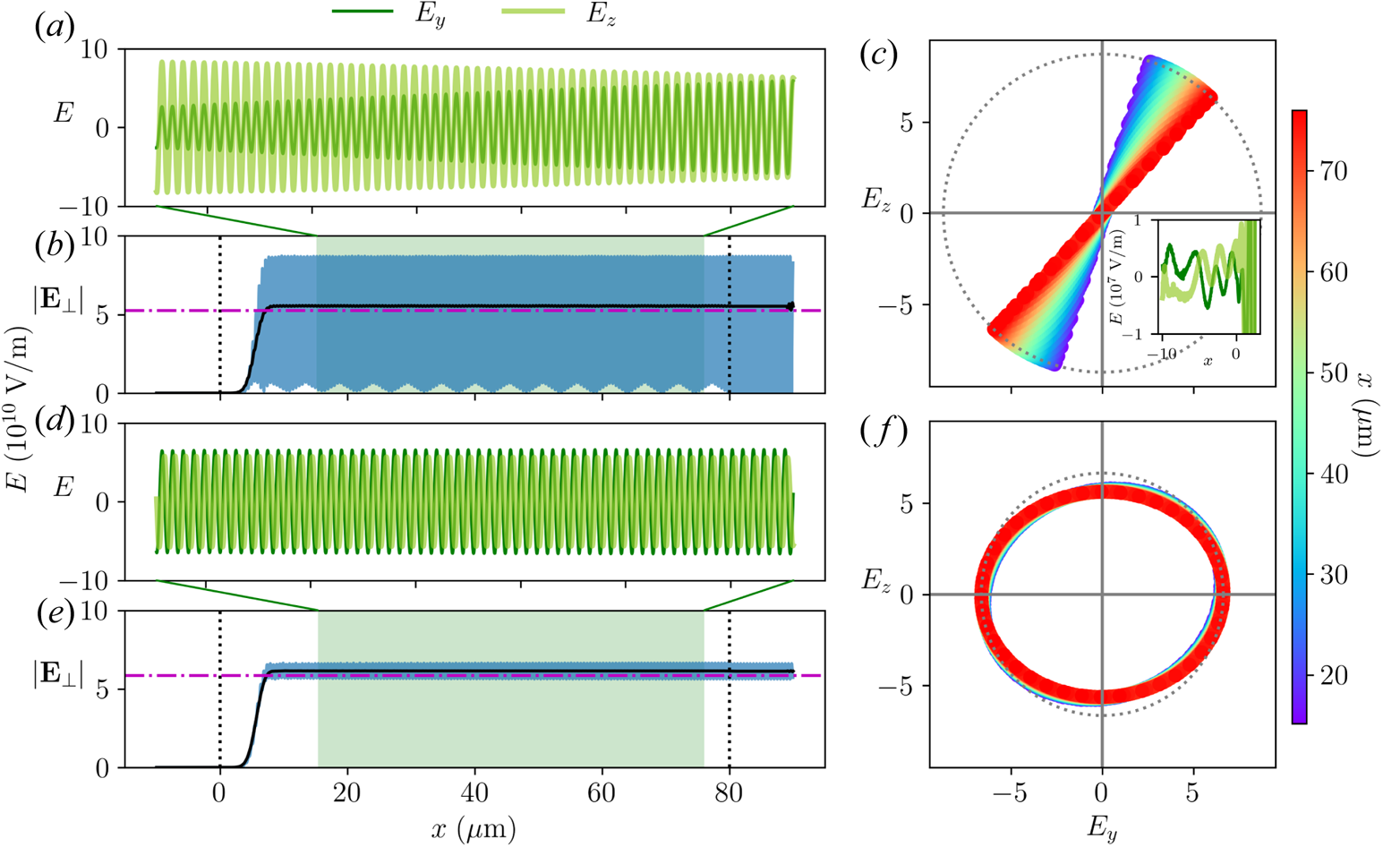
Figure 5. By launching a linearly polarised pump laser and fitting its $E_y$ (dark green) and $E_z$
 (light green) components (a) within the data region (b), polarisation angles of numerical eigenmodes can be determined. While the polarisation vector slowly rotates for none eigenmodes (c) as the wave propagates in $x$
 (colour scale), it remains close to a constant ellipse ( f) when an eigenmode is launched, whose field components have constant amplitude (d) within the data region $(e)$
 . The vertical dashed black lines in (b,e) mark the initial plasma–vacuum boundaries. The green shaded region is selected based on criteria that it is $4\lambda$
 within the boundaries, $8\lambda$
 behind the wave front and that the $2\lambda$
 -running average of $|\boldsymbol {E}_\perp |$
 (black) ramps above $95\,\%$
 of its average (magenta). The inset in (c) shows the noise level before the pump arrives, which is consistent with expected PIC noise when $T_0=10$
 eV. The polarisation rotation is consistent with $B_0=3$
 kT and $\theta _B=30^\circ$
 . The pump intensity is $I_1=10^{15}\,{\rm W}\,{\rm cm}^{-2}$
 .
.
With the simulation set-up and general considerations discussed above, technical details are elaborated below with examples, and the data analysis protocol is summarised in Shi (Reference Shi2022a). All reported results use the resolution of $40$ cells per pump laser wavelength and $N=100$
 particles per cell. Increasing or decreasing these parameters by a factor of two does not significantly change results. A larger plasma and simulation box increases the vulnerability to spontaneous pump scattering, which first shows up as unwanted oscillations on the right plasma boundary. On the other hand, using a much smaller plasma starts to violate $L_p\gg \lambda _1$
 , which is required in order for the slowly varying amplitude approximation to be valid.
3.1. Launching linear eigenmodes
As three-wave equations describe amplitudes of linear eigenmodes, the lasers need to be launched with specified polarisations to excite targeted eigenmodes only. Although polarisation matching is trivial for unmagnetised plasmas, where the two electromagnetic eigenmodes are degenerate, special care needs to be taken in magnetised cases where the R and L elliptically polarised eigenmodes are non-degenerate. If the polarisation is not matched properly, both R and L waves will be excited, giving rise to four polarisation combinations with different couplings (Shi & Fisch Reference Shi and Fisch2019). As incident lasers are purely transverse in the vacuum region, only the perpendicular components need to be matched with plasma eigenmodes. Denoting $\psi$ the elliptical polarisation angle and $\theta$
 is the wave phase,

where $\hat {\boldsymbol {y}}$ and $\hat {\boldsymbol {k}}$
 are unit vectors. The expression is symmetric about the $x$
 –$z$
–$z$ plane where $\boldsymbol {B}_0$
 lies. The special value $\psi =0$
 means that the wave is linearly polarised along $\hat {\boldsymbol {k}}\times \hat {\boldsymbol {y}}$
 , whereas $\psi ={\rm \pi} /2$
 means linear polarisation along $\hat {\boldsymbol {y}}$
 , $\psi ={\rm \pi} /4$
 is R circular polarisation about $\hat {\boldsymbol {k}}$
 and $\psi =-{\rm \pi} /4$
 is L circular polarisation.
Due to numerical dispersion and PIC density fluctuations, the polarisation angles of numerical eigenmodes are slightly different from analytic results. Launching waves with analytical $\psi$ leads to a small but sometimes observable polarisation rotation of $\boldsymbol {E}_\perp$
 , revealing contaminations from the unintended eigenmode. To determine $\tilde {\psi }$
 for numerical eigenmodes, a calibration step is performed where a linearly polarised wave at frequency $\omega$
 is launched with a constant $\boldsymbol {E}_\perp$
 , which lies along the diagonal of $y$
 –$z$
–$z$ plane. In most cases, this wave has large overlaps with both numerical eigenmodes, so


have unknown amplitudes $E_R$ and $E_L$
 and numerical wave vectors $\tilde {k}_R$
 and $\tilde {k}_L$
 are close to their analytical values $k_R$
 and $k_L$
 . The phases $\theta _R$
 and $\theta _L$
 vary deterministically with $\omega t$
 , but the initial phases depend on the unknown expansion coefficients when spanning the wave in terms of the eigenmodes. Note that each electric-field component is of the form $E=\mathcal {E}_R(\sin \tilde {k}_Rx \cos b_R + \cos \tilde {k}_Rx \sin b_R) + \mathcal {E}_L(\sin \tilde {k}_Lx \cos b_L + \cos \tilde {k}_Lx \sin b_L)$
 , where $b=\theta$
 for $E_y$
 and $b=\theta +{\rm \pi} /2$
 for $E_z$
 . By fitting a region of the simulation data where the wave envelopes are constant, as shown by the example in figure 5, the unknown amplitudes $\mathcal {E}_R$
 and $\mathcal {E}_L$
 , as well as the unknown phases $\theta _R$
 and $\theta _L$
 , can be determined by linearly regressing $\boldsymbol {E}_\perp (x)$
 against a four-dimensional basis $(\sin \tilde {k}_Rx, \cos \tilde {k}_Rx, \sin \tilde {k}_Lx, \cos \tilde {k}_Lx)$
 . In practice, the values of $\tilde {k}_R$
 and $\tilde {k}_L$
 are not easily known, so they are determined numerically by minimising the residual of linear regression using $k_R$
 and $k_L$
 as initial guesses. Finally, using $\mathcal {E}_{y}=E\sin \tilde {\psi }$
 and $\mathcal {E}_{z}=E\cos \tilde {\psi }$
 from the best fit, the polarisation angles $\tilde {\psi }$
 of numerical eigenmode is computed. In most cases, $\tilde {\psi }$
 is close to the analytical $\psi$
 . However, outliers can occur in limiting cases, such as when $B_0\rightarrow 0$
 where the degeneracy is week, or when $\theta _B\rightarrow 90^\circ$
 where the ellipticity is weak. In outlier cases, it is usually sufficient to launch the desired eigenmode using $\psi$
 , which is calculated using the code in Shi (Reference Shi2022b).
To verify that only the intended eigenmode is launched and to measure its transmitted amplitude, pump-only and seed-only eigen-runs are performed, where one laser is launched with numerically determined polarisation angle $\tilde {\psi }$ and the other laser is turned off completely. Example transverse fields $E_y(x)$
 and $E_z(x)$
 are plotted in figure 5. When the wave is not an eigenmode (figure 5c), the polarisation trajectory precesses. On the other hand, when the wave is close to an eigenmode, its trajectory is near a stationary polarisation ellipse. In figure 5( f), a slow precession can still be observed, but the contamination from the other eigenmode is small enough that it is not a major source of error. Using the pump-only eigen-run, the transmitted pump amplitude can be measured from data shown in figure 5(d). The transmitted amplitude is normalised by analytical wave energy coefficient to compute $a_1$
 , which enters $\gamma _0$
 via (2.4). Combining with the analytical $\varGamma$
 , the expected growth rate is computed to compare with simulations.
In the following, we focus on eigenmodes that are right-handed with respect to the magnetic field, which usually have the largest pump–seed coupling among the four possible polarisation combinations. When $\cos \theta _B>0$ , meaning that $\boldsymbol {B}_0$
 points towards $+x$
 , the seed laser is right-handed with respect to its wave vector. On the other hand, because the pump laser propagates in $-x$
 direction, the eigenmode is left-handed with respect to its wave vector. Another way to describe the mode selection is that at a given wave frequency $\omega$
 , the eigenmode with smaller $k$
 will be launched. This mode has an electric-field vector that corotates with the gyrating electrons and is therefore more strongly coupled with the electron-dominant plasma waves, such as the Langmuir-like P wave and electron-cyclotron-like F wave.
3.2. Extracting pump and seed envelopes
In stimulated runs where both pump and seed eigenmodes are turned on, we need to separate their contributions from the total electromagnetic fields, which are what PIC simulations observe directly. A plausible way of separating the waves is to use Fourier-like filters. However, because the pump and seed envelopes evolve in space–time due to three-wave interactions, their line shapes have long tails. Attempting to filter waves in the Fourier space and then taking inverse transform often introduce spurious oscillations. As an alternative approach, the pump and seed are directly separated in the configuration space using both electric- and magnetic-field data. Due to Faraday's law in one spatial dimension, wave fields are related in simple ways. For a right-propagating wave, $B_y=-E_z/v$ and $B_z=E_y/v$
 , where $v=\omega /k>0$
 is the phase velocity of the wave. On the other hand, for a left-propagating wave, $B_y=E_z/v$
 and $B_z=-E_y/v$
 have the opposite signs. When the signal contains a single right $(+)$
 and left $(-)$
 waves at constant amplitudes, the electric fields can be decomposed as $E_y = E^+_{y} +E^-_{y}$
 and $E_z = E^+_{z} + E^-_{z}$
 , and the magnetic fields are $B_y = -E^+_{z}/v_+ + E^-_{z}/v_-$
 and $B_z = E^+_{y}/v_+ - E^-_{y}/v_-$
 . Note that the right and left waves likely have different phase velocities $v_+$
 and $v_-$
 . After removing static components of $\boldsymbol {B}_0$
 , the wave fields satisfy
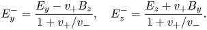
Reconstructions using the above Faraday filter are exact for constant-amplitude waves if $v_+$ and $v_-$
 are known. However, due to numerical dispersion and PIC noise, $v_\pm$
 differ slightly from analytical values, causing leakage through the Faraday filter.
To reduce the leakage, a calibration step is performed to determine the numerical phase velocities. Summing data of a pump-only run with data of a seed-only run before the wave fronts reach the opposite plasma boundary, $\tilde {v}_+$ and $\tilde {v}_-$
 are fitted using (3.3). The data are selected within the plasma region using similar criteria as in figure 5. The best-fit residuals are typically orders of magnitude smaller than the signals but a few times above the PIC noise level, as shown by the example in figure 6. The coherent errors are likely due to how electric- and magnetic-field data are combined. Note that when solving Maxwell's equations using a Yee-like mesh, transverse electric fields are discretised on cell boundaries whereas transverse magnetic fields are discretised on cell centres. Therefore, interpolations are needed before $B_{i\pm 1/2}$
 can be summed with $E_i$
 . Here, a simple linear interpolation is used to estimate $B_{i}\approx (B_{i-1/2} + B_{i+1/2})/2$
 , which is likely the leading cause of coherent errors. Using interpolation schemes that better match the PIC algorithm may further reduce the coherent error.
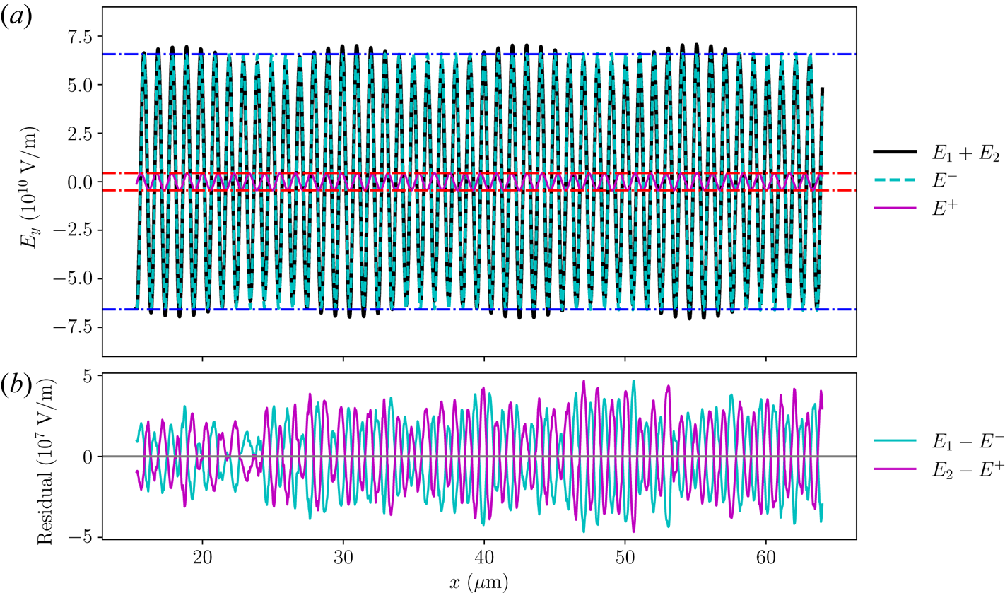
Figure 6. (a) The optimal phase velocities for separating the right ($+$ ) and left ($-$
 ) propagating waves are fitted using calibration data (black), which is the sum of a pump-only ($E_1$
 ) and a seed-only ($E_2$
 ) runs before the laser reaches the opposite plasma boundary. The amplitudes of the pump (dashed blue) and seed (dashed red) are known, and the fitting minimises the total difference between known and extracted pump (cyan) and seed (magenta) amplitudes. (b) The best-fit residuals are orders of magnitude smaller than the signals. However, the residuals have coherent leakages that are a few times larger than the PIC noise level. Fitting results for other field components are similar. The intensities are $I_1=10^{15}\,{\rm W}\,{\rm cm}^{-2}$
 and $I_2=5\times 10^{12}\,{\rm W}\,{\rm cm}^{-2}$
 .
.
However, other leakage sources are more important when the calibrated Faraday filter is applied to data from stimulated runs. Note that the simple relation between $\boldsymbol{E}$ and $\boldsymbol{B}$
 assumes plane waves with constant amplitudes. When the amplitude varies, additional terms arise, which depends on derivatives of the amplitude. In regimes where the amplitude varies slowly, these additional terms are small compared with the leading term but are large compared with the error from interpolation. Moreover, due to reflection and spontaneous scattering in PIC simulations, waves other than the pump and seed are present in the system, leading to even larger errors. For example, the pump laser reflects from the left plasma–vacuum boundary and propagates towards right together with the seed laser. Typically, the reflected pump amplitude is ${\sim }0.5\,\%$
 of the incident amplitude, which is ${\sim }7\,\%$
 of the seed amplitude when $I_1/I_2=200$
 . The Faraday filter is far from ideal for separating co-propagating waves, especially when they have comparable phase velocities. The leakage leads to spurious oscillations of the seed envelope, which are nevertheless usually less severe than caused by Fourier filters.
Having separated out pump and seed electric fields, the next step is to extract the wave envelopes that enter the three-wave equations. For a wave with slowly varying envelope, its electric field is $E(x)=\mathcal {E}(x)\sin (kx+b)+\epsilon (x)$ , where $\epsilon$
 is an error field. The envelope $\mathcal {E}(x)$
 can be estimated by mixing $E(x)$
 with a sinusoidal reference, which gives $E(x) \sin (kx+b') = \frac {1}{2}\mathcal {E}(x)[\cos (b-b')-\cos (2kx+b+b')]+\epsilon (x)\sin (kx+b')$
 . Averaging the mixed signal over $\lambda =2{\rm \pi} /k$
 ideally eliminates the last two terms to give

The reference phase $b'$ is scanned to maximise the norm of the average, which is attained when the phases are matched $b'=b$
 up to integer multiples of ${\rm \pi}$
 . Compared with a simple moving average, the above lock-in scheme reduces sensitivities to PIC noise and coherent errors. The numerical wave vector $\tilde {k}$
 , which is determined when fitting (3.2), is used to generate the sinusoidal reference. Moreover, to better remove the unwanted terms using the $\lambda$
 average, a matching grid $\tilde {x}_i$
 with spacing $\lambda /n$
 is used, where the integer $n=\lceil \lambda /\Delta x\rceil$
 and $\Delta x$
 is the original spacing of the PIC grid $x_i$
 . The reference is generated on grid $\tilde {x}_i$
 and mixed with $E(\tilde {x}_i)$
 , which is estimated from $E(x_i)$
 using linearly interpolation. Averaging over $\lambda$
 down samples the data, so the envelope $\mathcal {E}(x)$
 lives on a grid that is more sparse than the $\tilde {x}_i$
 grid by a factor of $n$
 . Note that due to their wavelengths difference, the pump and seed envelopes live on two separate grids. In addition to the transverse components, the $\mathcal {E}_x$
 component is estimated using the lock-in scheme alone, without attempting to separate right and left contributions. The longitudinal component is small but non-zero when lasers propagate obliquely with $\boldsymbol {B}_0$
 . Combining all components, the total scalar wave envelope $\mathcal {E}=|\boldsymbol{\mathcal{E}}|$
 is determined. Typical results of envelope extraction are shown in figure 7 for the $E_y$
 component. Results are similar for the $E_z$
 component, but are more noisy for the much smaller $E_x$
 component. The procedure successfully separates out the pump and seed lasers, and identifies their envelopes that enclose fast-oscillating fields.
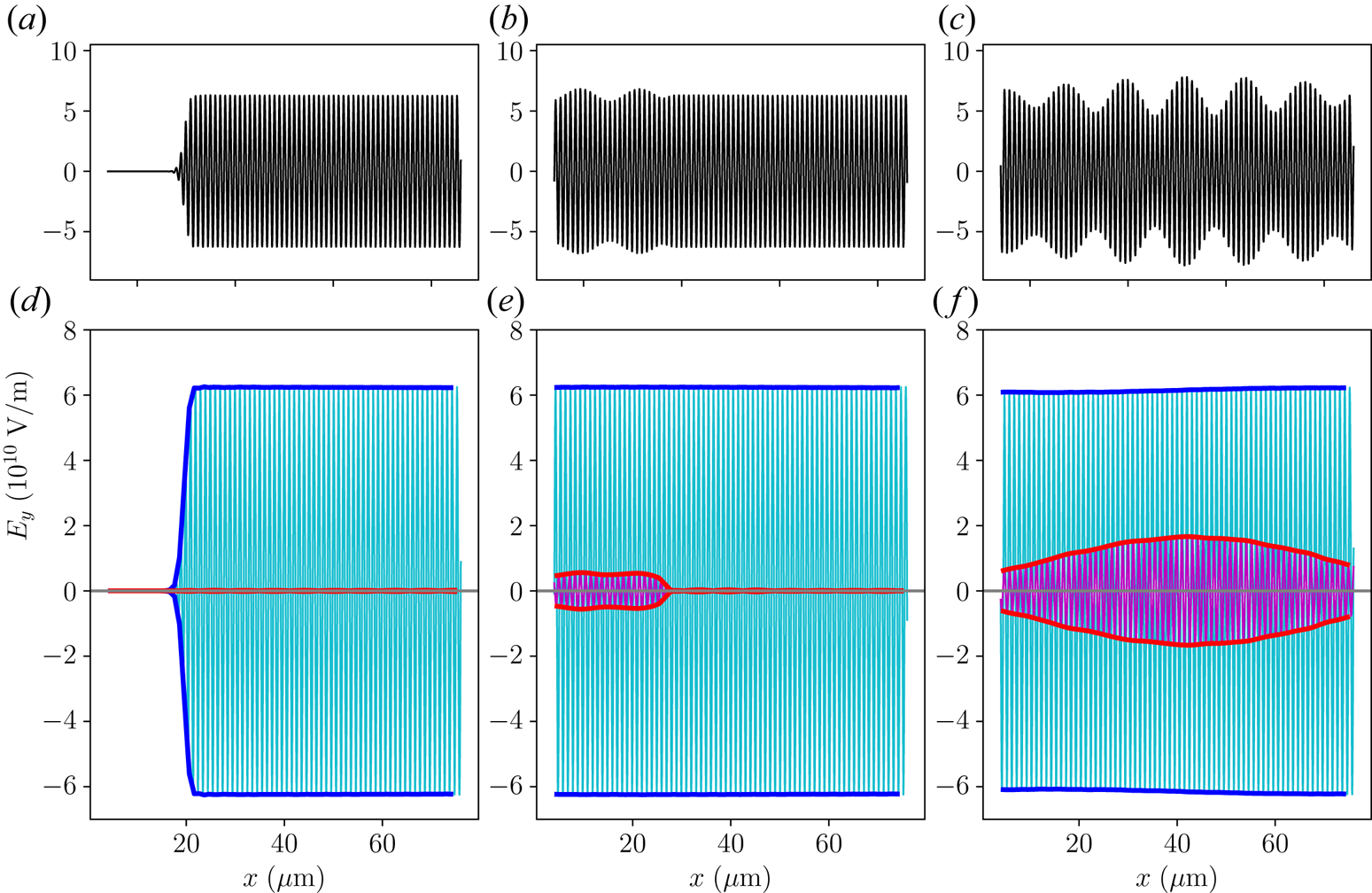
Figure 7. Raw data (a–c) is separated using a Faraday filter into pump (cyan) and seed (magenta) contributions (d–f), and envelopes of pump (blue) and seed (red) are extracted using a lock-in scheme. At $t\approx 0.25$ ps (a,d), the pump almost reaches the left plasma boundary and the seed has not entered. At later time $t\approx 0.48$
 ps (b,e), the pump fills the plasma and the seed enters from the left. At final time $t\approx 0.67$
 ps (c, f), the seed exits the right boundary and experiences noticeable growth, and the pump is slightly depleted. In this example, $T_0=10$
 eV, $B_0=3$
 kT, $\theta _B=30^\circ$
 , $I_1=10^{15}\,{\rm W}\,{\rm cm}^{-2}$
 and $I_2=5\times 10^{12}\,{\rm W}\,{\rm cm}^{-2}$
 . The interaction is mediated by a P wave and the resonant seed wavelength in vacuum is $\lambda _2\approx 1.09\,\mathrm {\mu }$
 m.
m.
3.3. Fitting data to analytical solutions
Before fitting extracted seed envelopes to analytical solutions, we need to ensure that the seed frequency is on resonance. Note that (2.1) is for resonant interactions that satisfy energy–momentum conservation $k^\mu _1=k^\mu _2+k^\mu _3$ where $k^\mu$
 is the wave 4-momentum. When phase-matching conditions are not satisfied, the waves can still interact, but a detuning term $\exp ({\rm i}x^\mu \delta k_\mu )$
 will appear in the three-wave equations. Analytical solutions in the detuned case are different from what is discussed in § 2, and usually exhibit less seed growth as a result of phase modulations. To determine the resonant $\omega _2^*$
 , the seed frequency is scanned near analytically expected resonances to maximise the growth of seed envelope $\mathcal {E}_2$
 in kinetic simulations. To reduce the requisite number of runs, only a few frequencies are simulated and $\hat {\mathcal {E}}_2(\omega _2)\propto [(\omega _2-\omega _2^*)^2+\mu ^2]^{-1}$
 is fitted using a Lorentzian profile. Here, $\hat {\mathcal {E}}_2$
 is the spatial maximum of $\mathcal {E}_2$
 at a given time slice and $\mu$
 is a phenomenological linewidth. In most cases, the fitting behaves as expected, as shown in figure 8(a). Using $\hat {\mathcal {E}}_2$
 at different time slices yields consistent estimates of $\omega _2^*$
 (dashed vertical lines), as long as $\mathcal {E}_2$
 has grown substantially above the noise level. In most cases, only nine $\omega _2$
 values are scanned within a $3\times 10^{13}$
 -rad s$^{-1}$
 window near the expected resonance. The fitting uses last four simulation outputs, when the seed has propagated across more than half the plasma length. The four estimates of $\omega _2^*$
 are averaged using equal weight to give a final estimate (solid vertical line). However, in some cases, more complicated spectra emerge during the scan, as shown in figure 8(b). In this example, $B_0=200$
 T and the electron gyro frequency is a few times smaller than the plasma frequency. In this regime, the kinetic wave dispersion relation involves multiple Bernstein-like waves near the expected warm-fluid resonance. In cases such as this, additional $\omega _2$
 values are scanned to resolve individual peaks, and only data near the expected resonance (solid circles) is used to fit $\omega _2^*$
 . Using data at multiple time slices again yields consistent estimates. As an intriguing observation, spacings between the side peaks do not seem to have a simple dependence on $B_0$
 and $\theta _B$
 , and often appears to change with time. These features remain to be investigated in the future.
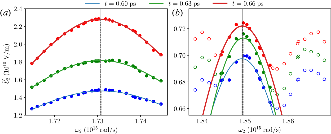
Figure 8. The spatial maximum of seed envelope $\hat {\mathcal {E}}_2$ is fitted to seed frequency $\omega _2$
 using a Lorentzian profile to determine the resonant seed frequency. (a) When $B_0=3$
 kT and the interaction is mediated by a P wave, the data matches a simple Lorentzian, and fittings using $\hat {\mathcal {E}}_2$
 at different time slices yield consistent results (dashed vertical lines), which is averaged to give a final estimate of $\omega _2^*$
 (solid vertical line). This is representative of what happens in most cases. (b) When $B_0=200$
 T and the interaction is mediated by an F wave, the data reveal multiple weak resonances. Data away from the expected warm-fluid peak are excluded from fitting (empty circles). The included data (solid circles) again yield consistent results across multiple time slices. In these examples, $T_0=10$
 eV, $\theta _B=30^\circ$
 , $I_1=10^{15}\,{\rm W}\,{\rm cm}^{-2}$
 and $I_2=5\times 10^{12}\,{\rm W}\,{\rm cm}^{-2}$
 .
.
Using a resonant seed to set up stimulated runs, the extracted seed envelopes are placed into analytic frame to prepare for fitting, as shown in figure 9. Note that in the step-function problem, the plasma–vacuum boundary is sharply at $x=0$ and a constant-amplitude seed arrives at the boundary when $t=0$
 . These idealised set-ups are necessarily softened in simulations, where the plasma expands into the vacuum forming a sheath region, and the seed is ramped up using a $\tanh$
 profile whose temporal width equals to the seed period to smooth out numerical artefacts. For the spatial axis, to avoid boundary effects, data within $4\lambda _1\gg \lambda _D$
 from the initial plasma–vacuum boundaries are excluded, where $\lambda _D$
 is the Debye length. Hence, the data frame $x_d$
 is shifted from the analytic frame $x_a=x_d+x_0$
 by an offset $x_0$
 . For the time axis, because the seed is launched after the pump has propagated across the plasma, the data frame $t_d$
 is delayed from the analytic frame $t_a=t_d-t_0$
 for some offset $t_0$
 . To place data into the analytic frame, the seed wave front $x_a=\tilde {v}_2t_a$
 is fitted to determine both offsets and the numerical group velocity $\tilde {v}_2$
 , which is close to but not equal to the analytical group velocity $v_2=\partial \omega /\partial k_x$
 due to numerical dispersions. The seed wave front is identified as the location where the seed envelope $\mathcal {E}_2$
 drops below half its boundary value, and the thickness of the wave front is identified as the spatial separation where $\mathcal {E}_2$
 attains $10\,\%$
 and $90\,\%$
 of its boundary value. Only data behind the wave front by twice its thickness are used for fitting. Finally, we need to normalise the electric field envelope $\mathcal {E}_2$
 . Note that the analytical solution of the step-function problem can be written in terms of the ratio $\alpha _2/h_0$
 , where $h_0$
 is the boundary value. In simulations, the value at the domain boundary is an input, but the value at the plasma–vacuum boundary is not controlled, because only a fraction of the incident seed laser is transmitted into the plasma. The boundary value inside the plasma is determined using the seed-only eigen-run. Using calibration data similar to what is shown in figure 5(d), the transmitted seed amplitude is measured and used to normalise envelopes in the stimulated run. Note that the calibration needs to be performed each time when plasma conditions are changed or the seed laser is varied.
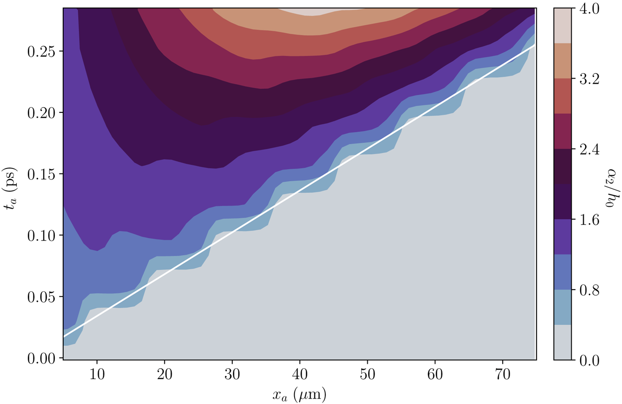
Figure 9. Normalised seed amplitude $\alpha _2/h_0$ in the analytical frame $(x_a, t_a)$
 . The step-like feature near the wave front is a visualisation artefact when only nine time slices are plotted. The wave front $x_a=\tilde {v}_2 t_a$
 (white line) is fitted to determine the numerical group velocity $\tilde {v}_2$
 . This example is the same run as in figure 7.
Having extracted $\alpha _2/h_0$ from the stimulated run, the data in the analytic frame are fitted to (2.27). Here, the simplification $v_3=0$
 is made because $|v_3|\ll v_2$
 . From figure 2, we see that $v_3=0$
 is already a good approximation even when $v_3=-v_2/10$
 . For a warm-fluid plasma with moderate temperature $T_0\sim 10$
 eV, the ratio $v_3/v_2\sim O(10^{-2})$
 is much smaller, so the limiting-form growth function provides an even better approximation. Evaluating the growth function requires a single numerical integral, which is much cheaper than computing the double integral in (2.25) that gives the exact solution at finite $v_3<0$
 . As another simplification, the physical collision module is turned off in PIC simulations, so lasers are undamped beyond spurious numerical collisions. Setting $\mu _2=0$
 gives $\Delta _2=\alpha _2/h_0-1$
 . The right-hand side of this expression is determined from simulation data to give $\tilde {\Delta }_2$
 , and the left-hand side is the analytical formula, which contains three parameters $v_2$
 , $\mu _3$
 and $\gamma _0$
 . As $\tilde {v}_2$
 is already determined from fitting the wave front, only two parameters remain to be fitted. The fitting is treated as an optimisation problem, where parameters are searched near their expected values to minimise the residual $\|\tilde {\Delta }_2-\Delta _2\|$
 , where $\|f\| = ({1}/{n_xn_t}) [\sum _{i=1}^{n_x}\sum _{j=1}^{n_t}|f(x_i,t_j)|^2]^{1/2}$
 . The discrepancy $\tilde {\Delta }_2-\Delta _2$
 is set to zero outside the region where data are valid. As discussed earlier, the data are valid when $x$
 is sufficiently far away from both the plasma boundaries and the seed front, and when $t$
 is after seed experiences noticeable growth but $a_1(x)$
 and $f_e(v_x)$
 remains largely unchanged. Typical best-fit results are shown in figure 10, where the simulation data (circles) are well matched by analytical solutions (lines), and the residuals are dominated by leakages during pump–seed separation.
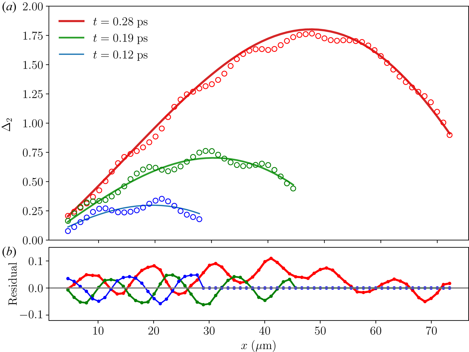
Figure 10. (a) The growth function extracted from simulation data (circles) is well matched by the analytical solutions (lines) using best-fit parameters. Results are shown for three representative time slices as the seed propagates and grows. The fitting quality at other time slices are similar. (b) Residuals of best fit are an order of magnitude smaller than the signal, and are dominated by leakage during pump–seed separation. The reflected pump amplitude is ${\sim }7\,\%$ of the seed. In this example, $T_0=100$
 eV, $B_0=3$
 kT, $\theta _B=30^\circ$
 , $I_1=10^{15}\,{\rm W}\,{\rm cm}^{-2}$
 , $I_2=5\times 10^{12}\,{\rm W}\,{\rm cm}^{-2}$
 and the interaction is mediated by a P wave. The best-fit parameters are $\tilde {v}_2\approx 2.97\times 10^8$
 m s$^{-1}$
 , $\tilde {\mu }_3\approx 5.17\times 10^{12}$
 rad s$^{-1}$
 and $\tilde {\gamma }_0\approx 9.25\times 10^{12}$
 rad s$^{-1}$
 .
.
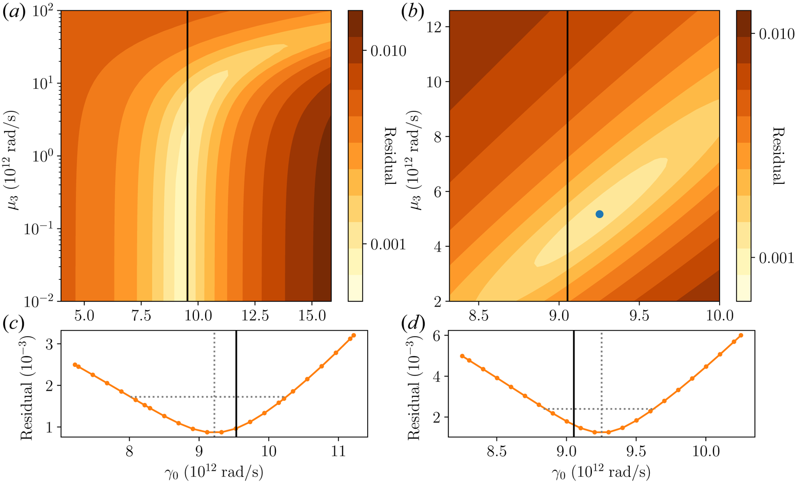
Figure 11. Uncertainties of fitting parameters are quantified by scanning the fit residual. (a,c) When $T_0=10$ eV is cold, damping is weak and poorly constrained. The best fit is far below the vertical scale and is consistent with a negligible $\mu _3$
 . Nevertheless, $\gamma _0$
 is well constrained and matches analytical growth rate (vertical solid line). (b,d) When $T_0=100$
 eV is hotter, damping becomes stronger. In this case, both $\gamma _0$
 and $\mu _3$
 are well constrained. The best fit (blue dot) matches the analytical growth rate within error bar, which is defined as the range where fit residual doubles its minimum. (c,d) Using the best fit $\mu _3$
 , a one-dimensional scan along $\gamma _0$
 gives marginal fit residuals and error bars (horizontal dashed line). In these examples, $B_0=3$
 kT, $\theta _B=30^\circ$
 , $I_1=10^{15}\,{\rm W}\,{\rm cm}^{-2}$
 , $I_2=5\times 10^{12}\,{\rm W}\,{\rm cm}^{-2}$
 and interactions are mediated by P waves. (b,d) are the same run as in figure 10.
To quantify uncertainty, the fit residual is scanned over a range of parameter values to estimate error bars. As parameters move away from their best-fit values, the fit residual increases. Error bars are defined as the parameter range beyond which the residual doubles its minimum. Using this definition, in the limit where data exactly match analytical solutions, the residual is zero and the error bar is also zero. In the opposite limit where simulation and theory poorly match, the residual is large and the error bar is wide. Two examples are shown in figure 11, where the resonant interactions are mediate by Langmuir-like P waves. When the temperature $T_0=10$ eV is cold (figure 11a), collisionless damping of the plasma wave is minuscule. In this case, the residual remains small for a wide range of $\mu _3$
 values, and the best fit is $\tilde {\mu }_3\approx 1.36\times 10^{-2}$
 rad s$^{-1}$
 , which is consistent with zero damping. On the other hand, the residual increases rapidly when $\gamma _0$
 deviates from its best-fit value $\tilde {\gamma }_0\approx 9.22\times 10^{12}$
 rad s$^{-1}$
 , which is close to the analytical value $\gamma _0^a\approx 9.53\times 10^{12}$
 rad s$^{-1}$
 (solid vertical line). The marginal error bar is shown in figure 11(c), where $\mu _3$
 is fixed at its best-fit value and $\gamma _0$
 is scanned. The residual is convex near $\tilde {\gamma }_0$
 (dashed vertical line) and $\gamma _0^a$
 is within the error bar (dashed horizontal line). When $T_0=100$
 eV is hotter (figure 11b), collisionless damping is stronger, so both $\gamma _0$
 and $\mu _3$
 are constrained. As discussed earlier, magnetised collisionless damping is not easy to compute, so the procedure here provides a unique method for measuring the damping rate, which in this case is best fitted by $\tilde {\mu }_3\approx 5.17\times 10^{12}$
 rad s$^{-1}$
 . The best-fit $\tilde {\gamma }_0\approx 9.25\times 10^{12}$
 rad s$^{-1}$
 matches the analytical value $\gamma _0^a\approx 9.05\times 10^{12}$
 rad s$^{-1}$
 within the marginal error bar shown in figure 11(d). The marginal residual is always convex and usually skewed towards smaller $\gamma _0$
 . The two-dimensional landscape of the residual is flat along a valley in the $\gamma _0$
 –$\mu _3$
 space. This is intuitive because a larger damping cancels the effect of a larger growth. In the asymptotic limit $t\rightarrow +\infty$
 , the exponential solution ${\rm e}^{\kappa x}$
 only depends on the ratio $\kappa =\gamma _0^2/\mu _3v_2$
 , so $\gamma _0$
 and $\mu _3$
 are not independently constrained. In other words, the separate constrains come from solutions at earlier time. As discussed after (2.27), the growth function $\Delta _2$
 is symmetric about $x=\frac {1}{2}v_2t$
 in the absence of damping. As $\mu _3$
 increases, the growth behind $x=\frac {1}{2}v_2t$
 is reduced more, leading to an asymmetric profile of $\Delta _2$
 . The asymmetry in the transient-time profile is what allows the effects of $\mu _3$
 and $\gamma _0$
 to be distinguished.
3.4. Scanning physical parameters
Having described in detail how simulations are set up and how data are processed, the protocol is applied to scan physical parameters and compare simulations with theory. First, it is useful to verify that the pump and seed intensities are selected properly. As discussed at the beginning of this section, the pump and seed intensities are constrained by ${10^{10}\,{\rm W}\,{\rm cm}^{-2}} \ll I_2\sim 10^{-2} I_1\ll {10^{14}\,{\rm W}\,{\rm cm}^{-2}}$ . Within this range, the bare growth rate $\gamma _0\propto a_1\propto I_1^{1/2}$
 scales with the pump intensity $I_1$
 but is independent of $I_2$
 . This theory prediction is confirmed by results shown in figure 12, where black lines are from the theory and orange symbols with error bars are simulation results. In figure 12(a), the seed intensity is fixed at $I_2=5\times 10^{12}\,{\rm W}\,{\rm cm}^{-2}$
 and the agreement is excellent within the range $I_1$
 is scanned. Note that the black line is not a fit of data. A hint of deviation can be seen from the last data point at $I_1=8\times 10^{15}\,{\rm W}\,{\rm cm}^{-2}$
 , where data start to drop below the theory line. This behaviour is expected because a pump that is too intense causes large spontaneous scattering that depletes the pump. Signatures of spontaneous scattering are clearly visible in the inset, which shows the Fourier power spectrum of transverse electric fields within the plasma region. At $I_1=5\times 10^{14}\,{\rm W}\,{\rm cm}^{-2}$
 (blue), the spectrum is clean and dominated by the pump and seed near $ck=2\times 10^{15}$
 rad s$^{-1}$
 and the plasma wave near $ck=4\times 10^{15}$
 rad s$^{-1}$
 . In comparison, at $I_1=8\times 10^{15}\,{\rm W}\,{\rm cm}^{-2}$
 (red), extra waves are excited due to spontaneous scattering. These extra waves remove energy that would otherwise be used to grow the seed, and they also constitute a messy background that jeopardises the data analysis. In figure 12(b), the agreement remains excellent within the range $I_2$
 is scanned, where the pump intensity is fixed at $I_1=10^{15}\,{\rm W}\,{\rm cm}^{-2}$
 . The error bars remain largely constant due to two competing effects. At stronger seed intensities, pump depletion occurs earlier so more data are excluded from fitting, resulting in fewer constraints and larger error bars. On the other hand, at weaker seed intensities, the leakage during pump–seed separation more severely distorts the seed profile, causing poorer fits and larger error bars. The two competing effects cause error bars to remain roughly constant within this $I_2$
 range. Effects of leakage can be clearly seen in the inset. The normalised envelope $\alpha _2/h_0$
 is relatively smooth when $I_2=10^{13}\,{\rm W}\,{\rm cm}^{-2}$
 (magenta), but the spurious oscillations become more severe when $I_2=6.25\times 10^{11}\,{\rm W}\,{\rm cm}^{-2}$
 (cyan). The artefacts are primarily due to reflected pump that copropagates with the seed, which cannot be separated using (3.3) and (3.4), causing spurious oscillations. Limited by these effects, simulations below use $I_1=10^{15}\,{\rm W}\,{\rm cm}^{-2}$
 and $I_2=5\times 10^{12}\,{\rm W}\,{\rm cm}^{-2}$
 .
.

Figure 12. The bare growth rate $\gamma _0\propto I_1^{1/2}$ scales with pump intensity (a) and is independent of the seed intensity (b) within the range where simulations are described by the linearised three-wave equations. Theory predictions (black lines) match simulation results (orange symbols) within error bars. At large pump intensity $I_1$
 , spontaneous scattering depletes the pump and excites additional waves, as shown in the inset of (a) where the Fourier power spectra are plotted for transverse electric fields within the plasma region. At larger seed intensity $I_2$
 , pump depletion occurs earlier, which reduces the amount of data that can be used for fitting analytical solutions. On the other hand, at smaller $I_2$
 , the leakage during pump–seed separation is more detrimental, as shown in the inset of (b) where the normalised envelopes $\alpha _2/h_0$
 suffer from spurious oscillations. In this set of scans, $T_0=10$
 eV, $B_0=3$
 kT, $\theta _B=30^\circ$
 , the vacuum seed wavelength is $\lambda _2\approx 1.088\,\mathrm {\mu }$
 m and the interaction is mediated by a P wave.
Second, the protocol is used to scan plasma temperature $T_0$ to determine the range of validity of warm-fluid theory (figure 13). At low temperature, collisionless damping of plasma waves are negligible and the $\mu _3$
 error bars are large. On the other hand, when $T_0>10^2$
 eV, damping starts to dominate growth and data start to deviate from warm-fluid theory. At $T_0\sim 10^3$
 eV, the seed barely grows unless the pump is stronger. However, a stronger pump suffers more from spontaneous scattering, leading to systematic errors and large uncertainties. Therefore, the applicability of the protocol does not far exceed the temperature range reported here. Within this range, the expected $\gamma _0$
 from warm-fluid theory (line) agrees with simulation data (squares) up to $T_0=300$
 eV, where hints of disagreements emerge. It is remarkable that even when collisionless damping has become significant, which is a purely kinetic phenomenon, the three-wave coupling remains well described by the warm-fluid theory. In subsequent scans, the plasma temperature is fixed at $T_0=10$
 eV where damping is negligible.
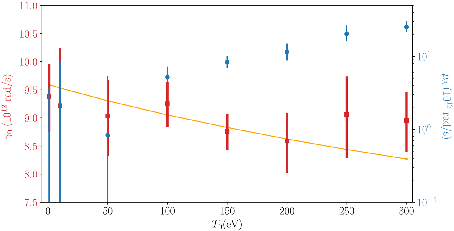
Figure 13. The growth rate $\gamma _0$ (left axis) and damping rate $\mu _3$
 (right axis) as functions of the plasma temperature $T_0$
 . Coloured symbols with error bars are simulation results and the orange line is the expected growth rate from warm-fluid theory. When $T_0$
 increases by tenfold, $\mu _3$
 increases by orders of magnitude. On the other hand, $\gamma _0$
 decreases only slightly, and data are well matched by theory until the last two points. In this set of scans, $B_0=3$
 kT, $\theta _B=30^\circ$
 , $I_1=10^{15}\,{\rm W}\,{\rm cm}^{-2}$
 , $I_2=5\times 10^{12}\,{\rm W}\,{\rm cm}^{-2}$
 and the interactions are mediated by P waves.
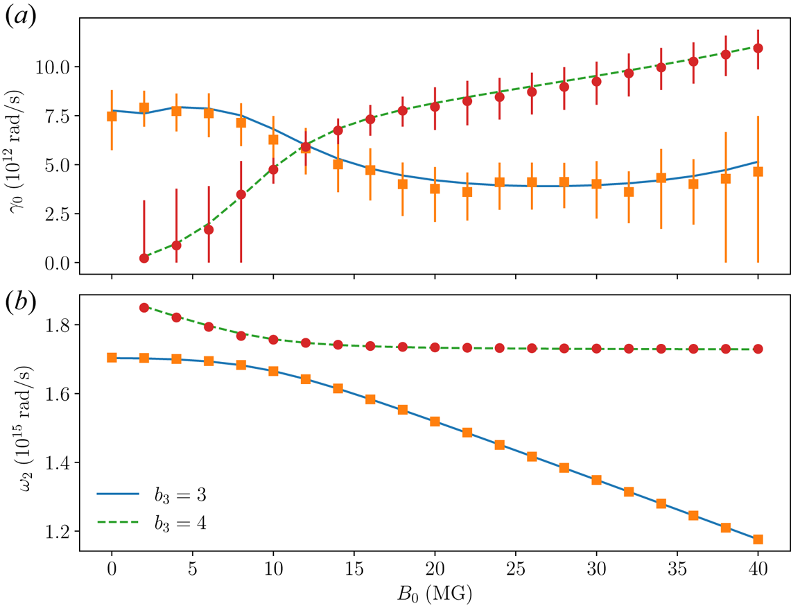
Figure 14. (a) Growth rate $\gamma _0$ and (b) resonant seed frequency $\omega _2$
 as functions of the background magnetic field $B_0$
 when interactions are mediated by electron-dominant P and F waves. Analytical results (lines) match simulation data (symbols). Error bars are shown for $\gamma _0$
 but are too small to show for $\omega _2$
 . The index $b_3$
 labels the wave branch of $\alpha _3$
 . For example, $b_3=4$
 means $\alpha _3$
 is the fourth highest-frequency branch of the warm-fluid dispersion relation. In this set of scans, $T_0 =10\ {\rm eV}$
 , $\theta _B=30^\circ$
 , $I_1=10^{15}\,{\rm W}\,{\rm cm}^{-2}$
 and $I_2=5\times 10^{12}\,{\rm W}\,{\rm cm}^{-2}$
 .
.

Figure 15. Same as figure 14, but for $\theta _B=\langle \boldsymbol {k},\boldsymbol {B}_0\rangle$ scan at fixed $B_0=3$
 kT.
kT.
Third, the protocol is used to scan the background magnetic field strength $B_0$ for interactions that are mediated by electron-dominant resonances (figure 14). In weak magnetic fields, the $b_3=3$
 resonance, namely, the $\alpha _3$
 eigenmode whose frequency is the third highest at a given wave vector, is the Langmuir-like P wave. In particular, at $B_0=0$
 , this resonance is precisely mediated by the Langmuir wave that gives rise to Raman backscattering in unmagnetised plasmas. When $B_0\ne 0$
 and $\theta _B\ne 0$
 , this eigenmode is modified due to cyclotron motion, but its frequency only weakly dependents on $B_0$
 , as shown in figure 14(b). Beyond $B_0\approx 10$
 MG, the eigenmodes cross over, and the $b_3=3$
 resonance becomes the electron-cyclotron-like F wave, whose frequency $\omega _3$
 increases almost linearly with $B_0$
 . Complementarily, the $b_3=4$
 resonance is the F wave in weak $B_0$
 and crosses over to become the P wave in strong magnetic fields. Within the $B_0$
 range scanned here, the interaction mediated by the F wave provides a smaller coupling than the P wave at the same $B_0$
 . In particular, at $B_0=0$
 , the F wave vanishes and provides zero coupling. The exception is near $B_0=10$
 MG when the two eigenmodes strongly hybridise. Although they remain two distinct eigenmodes, their couplings during frequency crossover become equal. Immediately after the crossover, P-wave coupling recovers its unmagnetised strength and continues to increase, whereas F-wave coupling drops before starting to increase again. In stronger fields not shown here, $\gamma _0$
 continues to increase and F-wave coupling surpasses P-wave coupling (Shi & Fisch Reference Shi and Fisch2019). In even stronger fields, the F-wave frequency approaches $\omega _1/2$
 and two-magnon decays are encountered (Manzo et al. Reference Manzo, Edwards and Shi2022), for which kinetic effects are dominant. After the F-wave frequency increases beyond $\omega _1/2$
 , it can no longer mediate resonant interactions, so only the P resonance remains. As $B_0$
 further increases, mediation by P wave continues to strengthen, and a strong resonance is encountered when electron gyro frequency approaches $\omega _1$
 (Edwards et al. Reference Edwards, Shi, Mikhailova and Fisch2019). Beyond that point, the 1-$\mathrm {\mu }$
 m pump frequency is below the R-wave cutoff, so only L-wave pump can propagate, whose coupling is substantially weaker. In the range scanned in figure 14, kinetic effects are not overwhelming and the agreement is excellent. Note that the lines are not fits of data. Although error bars for $\gamma _0$
 can perhaps be reduced, growth rates extracted from simulations already match detailed features of analytical predictions.
Finally, the protocol is used to scan $\theta _B$ , the angle between the magnetic field and the wave vectors, when interactions are mediated by the two highest-frequency resonances (figure 15). The magnetic field is fixed at $B_0=3$
 kT, where the electron cyclotron frequency is larger than the plasma frequency. In this case, the $b_3=3$
 resonance is the electron-cyclotron wave when $\theta _B=0$
 and becomes the UH wave when $\theta _B=90^\circ$
 . The other resonance with branch index $b_3=4$
 is the Langmuir wave when $\theta _B=0$
 and becomes the LH wave when $\theta _B=90^\circ$
 . The coupling provided by the electron-cyclotron wave is zero, because the interaction is both polarisation forbidden and energy forbidden (Shi et al. Reference Shi, Qin and Fisch2018). The coupling provided by the LH wave is finite, but smaller than UH mediation by a factor that is roughly proportional to $(\omega _{\mathrm {LH}}/\omega _{\mathrm {UH}})^{1/2}\ll 1$
 (Shi et al. Reference Shi, Qin and Fisch2017b). On the other hand, the coupling provided by the electron-dominant UH wave is strong, and has a comparable strength as unmagnetised Raman scattering. As $\theta _B$
 increases, the hybridisation between cyclotron motion and electrostatic oscillation changes. The growth mediated by the $b_3=3$
 resonance increases, whereas the growth mediated by the $b_3=4$
 resonance decreases. The simulation data (symbols) and analytical results (lines) agree within error bars. Note that the lines are not fits of data. The data point at $b_3=4$
 and $\theta _B=90^\circ$
 is missing because the LH coupling is too weak and the resonance cannot be unambiguously identified.
4. Discussion
Although strong resonances can be fitted using the protocol described in this paper, weak resonances are challenging to extract. In warm-fluid plasmas, weak resonances include the LH wave, as well as sound-like waves, Alfvén-like waves and ion-cyclotron-like waves. In these resonances, ion motion is important, so the coupling are typically smaller than electron-dominant modes by factors proportional to $1/\sqrt {M_i}\ll 1$ . Weak resonances are difficult to isolate because they compete with much stronger spontaneous scattering in PIC simulations. Within the limited time window before spontaneous scattering overwhelms simulation results, the stimulated scattering mediated by a weak resonance barely experiences any growth, and is therefore difficult to observe amidst leakages during pump–seed separation.
The difficulties may be circumvented in a number of ways. First, numerical noise can be reduced to suppress unphysical spontaneous scattering. This can be achieved using less-noisy Vlasov simulations. However, Vlasov codes can be expensive when an oblique background magnetic field is present, because the simulations need to include at least one spatial dimension and three velocity directions. Alternatively, PIC simulations with a substantially larger number of particles $N$ can be used to reduce numerical fluctuations. However, this can also be expensive because PIC noise only decreases slowly with $\sqrt {N}$
 . Second, plasma parameters can be chosen in regimes where electron modes are strongly damped or chirped. For example, at kiloelectronvolt temperature that is relevant for fusion, collisionless damping rates for electron modes are stronger than the growth rates. In comparison, due to heavy ion masses, ion-dominant modes are less damped. The balance between damping and growth can make ion-dominant modes competitive with electron-dominant modes, and therefore survive numerical artefacts. It remains to be seen whether couplings predicted by warm-fluid theory are reliable in regimes where kinetic effects are expected to be important.
In addition, nonlinear solutions of the three-wave equations can be used to fit simulations, which allow the seed intensity to be much stronger such that stimulated scattering dominates spontaneous scattering. The three-wave equations are nonlinear partial differential equations, which are difficult to solve analytically. Nevertheless, in some cases, analytical solutions may be obtained using the inverse scattering method (Kaup, Reiman & Bers Reference Kaup, Reiman and Bers1979), and the set-up might be possible to realise in kinetic simulations. Moreover, numerical solutions of the three-wave equations can be used to fit kinetic simulations. Note that analytical solutions of wave-like equations are typically given in integral form, which may not have simple closed-form expressions. Even for the linearised three-wave problem, the integrals need to be evaluated numerically, except for a few limiting cases. The necessity of numerical integration makes it appealing to bypass analytical steps to directly solve the nonlinear equations using numerical methods. Parameters such as the coupling coefficient may be scanned such that numerical solutions of three-wave equations match kinetic simulations, which involve many more variables. Once the analytical formula for magnetised coupling coefficient is benchmarked, the much cheaper numerical solutions can be used in lieu of the much more expensive kinetic simulations to study three-wave interactions of interest.
Finally, interactions in higher spatial dimensions remain to be investigated, which involves additional physics that are important for magnetised inertial confinement fusion and can also be exploited as a technique to reduce numerical artefacts. For example, during cross-beam energy transfer, the pump and seed lasers propagate in different directions. When a background magnetic field is present in yet another direction, the interaction is intrinsically multidimensional. After Lorentz boost into a reference frame where the two lasers are counter propagating, the plasma has a background flow and the static magnetic field partially transforms into an electric field. However, the initial boundary value problem in a finite plasma slab is more difficult to transform. In this case, higher-dimensional simulations are conceptually simpler even though they are more costly. In addition, using extra spatial dimensions, pump and seed may become easier to separate. Note that the reflected laser propagates at the specular angle. If the seed is at a different angle, then it can be separated from the reflected pump, which is difficult to achieve in one spatial dimension. Using the different propagation angles, contamination from spontaneous scattering may also be mitigated. In unmagnetised plasmas, spontaneous scattering is usually strongest in the backward direction. Although magnetisation changes the preferred scattering angle, there is usually a direction where spontaneous scattering peaks. Away from that direction, the seed laser suffers less from spontaneous scattering, so weak resonances may then become extractable.
In summary, this paper derives analytical solutions of the linearised three-wave equations in one spatial dimension, and use the solutions to benchmark magnetised coupling coefficients predicted by warm-fluid theory. A protocol is developed to set up, calibrate and process PIC simulations, so that simulation data can be fitted to analytical solution in the same set-up. The rigorous protocol yields excellent agreement between theory and simulations in the backscattering geometry for a wide range of plasma temperature $T_0$ , magnetic field strength $B_0$
 and propagation angle $\theta _B$
 . Growth rates predicted by warm-fluid theory match fully kinetic simulations even when collisionless damping becomes significant. The protocol is applicable to strong resonances that suffer less from spontaneous scattering and pump–seed leakage. It remains to be investigated whether the agreement can be extended to weaker resonances and to higher temperatures.
Acknowledgements
The author thanks D.J. Strozzi, P.A. Michel, T. Chapman and J.D. Moody for helpful discussions.
Editor Dmitri Uzdensky thanks the referees for their advice in evaluating this article.
Funding
This work was performed under the auspices of the US Department of Energy by Lawrence Livermore National Laboratory under Contract DE-AC52-07NA27344 and is supported in part by LLNL-LDRD under Project Number 20-SI-002. The EPOCH code used in this work was in part funded by the UK EPSRC grants EP/G054950/1, EP/G056803/1, EP/G055165/1, EP/ M022463/1 and EP/P02212X/1.
Declaration of interests
The author reports no conflict of interest.
Data and code availability
Data underlying figures in this paper are openly available in zenodo at https://doi.org/10.5281/zenodo.7126300, reference (Shi Reference Shi2022c). The PIC simulations are performed using version 4.17.10 of the EPOCH code at https://github.com/Warwick-Plasma/epoch, reference (Arber et al. Reference Arber, Bennett, Brady, Lawrence-Douglas, Ramsay, Sircombe, Gillies, Evans, Schmitz and Bell2015). The analytical three-wave coupling coefficients from warm-fluid theory are evaluated using version 2.2.0 of the Three-Wave-MATLAB code at https://gitlab.com/seanYuanSHI/three-wave-matlab, reference (Shi Reference Shi2022b). The protocol for computing analytical solutions, setting up simulations and analysing data is summarised at https://gitlab.com/seanYuanSHI/linear-three-wave-analysis/, reference (Shi Reference Shi2022a).
Appendix A. Solution map of the coupled-mode equation
In this appendix, we evaluate the Fourier integral in (2.14) and analyse properties of $\it{\boldsymbol{\varPhi}}$ in (2.15), which gives the solution map of the linear differential operator $\it{\boldsymbol{\mathsf{L}}}$
 in (2.3). We focus on the non-degenerate case $\Delta v=v_2-v_3>0$
 .
.
The coupled-mode equation $\it{\boldsymbol{\mathsf{L}}}\boldsymbol {\alpha }=\boldsymbol {0}$ can be mapped to the standard wave equation. Using the transformed coordinates given by (2.12), the advective derivatives become $\partial _t+v_2\partial _x=\frac {1}{2}\Delta v(\partial _\tau +\partial _z)$
 and $\partial _t+v_3\partial _x=\frac {1}{2}\Delta v(\partial _\tau -\partial _z)$
 . Moreover, after changing variable $\boldsymbol {\alpha }=\rho \boldsymbol {\beta }$
 , where $\rho$
 is given by (2.13), the damping terms are removed and
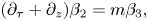
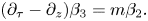
Substituting one equation into the other, $\boldsymbol {\beta }$ satisfies $(\partial _\tau ^2-\partial _z^2-m^2)\boldsymbol {\beta }=\boldsymbol {0}$
 , which is the Klein–Gordon equation with an imaginary mass term. As the equation is invariant under Lorentz transformations, it can be solved in any inertial frame.
Using Lorentz transformations, we can evaluate the integral in (2.14) in the complex $k'$ plane in three space–time regions. First, when $(\tau,z)$
 is a space-like separation, namely $|\tau |<|z|$
 , we can Lorentz boost into a reference frame where $\tau '=0$
 . In this frame, the integrand is zero, so $g=0$
 . Transforming back to the original frame
which enforces the causality that information outside the light cone does not contribute to the solution. Second, when $(\tau,z)$ is a time-like separation, namely $|\tau |>|z|$
 , we can Lorentz boost into a reference frame where $z'=0$
 . The direction of time is preserved if $\tau '=\pm \sqrt {\tau ^2-z^2}$
 takes the same sign as $\tau$
 . Then, the integrand becomes an even function and $g(\tau '/m)=({1}/{{\rm \pi} })[\int _0^1 {\rm d}\zeta \sinh (\tau '\sqrt {1-\zeta ^2})/\sqrt {1-\zeta ^2} + \int _1^{+\infty }{\rm d}\zeta \sin (\tau '\sqrt {\zeta ^2-1})/\sqrt {\zeta ^2-1}]$
 . Changing the variable to $\zeta =\sqrt {1+\chi ^2}$
 , the second integral equals the imaginary part of $\int _0^{+\infty }{\rm d}\chi \exp ({{\rm i}\tau '\chi })/\sqrt {1+\chi ^2}$
 . As the integrand is analytic away from the branch cut, the contour can be closed to become an integral along the imaginary $\chi ={\rm i}\eta$
 axis, as shown in figure 16. When $\tau '>0$
 , $\exp ({{\rm i}\tau '\chi })$
 decays when $\eta >0$
 , so the closure is in the first quadrant. For $\eta \in (1,\infty )$
 , the integral is real, so the only contribution comes from $\eta \in [0,1)$
 , which gives the imaginary part as $\int _0^1 {\rm d}\eta \exp ({-\tau '\eta })/\sqrt {1-\eta ^2}$
 . Substituting this into $g(\tau '/m)$
 and changing variable $\zeta =\sqrt {1-\eta ^2}$
 in the first integral, we have $g(\tau '/m)=({1}/{{\rm \pi} })\int _0^1 {\rm d}\eta \cosh (\tau '\eta )/\sqrt {1-\eta ^2}=\frac {1}{2}I_0(\tau ')$
 , where $I_0$
 is modified Bessel function (DLMF 2022, (10.32.2)). Similarly, when $\tau '<0$
 , the contour integral is closed in the fourth quadrant, giving rise to an overall negative sign. In the original frame,

Finally, for light-like separation $|\tau |=|z|$ , $\exp ({{\rm i}k'z})=\cos k'\tau \pm {\rm i}\sin k'\tau$
 . As $\hat {g}(k')$
 is an even function, $g(z=\pm \tau /m)=({1}/{{\rm \pi} })[\int _0^1 {\rm d}\zeta \cos (\tau \zeta )\sinh (\tau \sqrt {1-\zeta ^2})/\sqrt {1-\zeta ^2} + \int _1^{+\infty } {\rm d}\zeta \cos (\tau \zeta )\sin (\tau \sqrt {\zeta ^2-1})/\sqrt {\zeta ^2-1}]$
 . Changing the variable to $\zeta =\sqrt {1+\chi ^2}$
 , the second integral equals the imaginary part of $\frac {1}{2}\int _0^{+\infty }{\rm d}\chi \{\exp [{\rm i}\tau (\sqrt {1+\chi ^2}+\chi )] - \exp [{\rm i}\tau (\sqrt {1+\chi ^2}-\chi )] \}/\sqrt {1+\chi ^2}$
 . As $\sqrt {1+\chi ^2}+\chi \simeq 2\chi$
 when $\chi \rightarrow \infty$
 , the contour can be closed in first quadrant when $\tau >0$
 to move the integral along $\chi ={\rm i}\eta$
 axis, as shown in figure 16. For $\eta \in (1,+\infty )$
 , the integral is real, so the only contribution comes from $\eta \in [0,1)$
 , which gives the imaginary part as $\int _0^1{\rm d}\eta \cos (\tau \sqrt {1-\eta ^2})\exp ({-\tau \eta })/\sqrt {1-\eta ^2}$
 . On the other hand, $\sqrt {1+\chi ^2}-\chi \simeq 1/2\chi$
 when $\chi \rightarrow \infty$
 , so closing the contour along $\chi =R\,{\rm e}^{{\rm i}\theta }$
 gives a finite boundary term ${\rm i}\int _0^{{\rm \pi} /2} {\rm d}\theta \, \chi \exp [{\rm i}\tau (\sqrt {1+\chi ^2}-\chi )]/\sqrt {1+\chi ^2} \rightarrow {\rm i}\int _0^{{\rm \pi} /2} {\rm d}\theta = {\rm i}{\rm \pi} /2$
 when $R\rightarrow \infty$
 . The imaginary part of the second $\chi$
 integral is therefore $-{\rm \pi} /2+\int _0^1{\rm d}\eta \cos (\tau \sqrt {1-\eta ^2})\exp(\tau \eta)/\sqrt {1-\eta ^2}$
 . Summing the two $\chi$
 integrals leads to a cancellation with the first $\zeta =\sqrt {1-\eta ^2}$
 integral, leaving a constant $\frac {1}{4}$
 . Similarly, when $\tau <0$
 , the contour integration is closed in the fourth quadrant, giving rise to an overall negative sign. Therefore, along the light cone
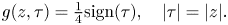
Using $I_0(0)=1$ and the definition of Heaviside step function with $\varTheta (0)=\frac {1}{2}$
 , the inverse Fourier transform in all space–time regions is combined into a single expression.
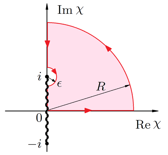
Figure 16. Contour integral in the complex $\chi$ plane. The integrands have a branch cut between $\chi =\pm {\rm i}$
 , but are otherwise analytic. As integrals along contours are zero, an integral along the real $\chi$
 axis can be moved to the imaginary $\chi ={\rm i}\eta$
 axis by closing the contour at $R\rightarrow \infty$
 and $\epsilon \rightarrow 0$
 . When $\tau >0$
 , the closure is in the first quadrant as shown in this figure, whereas when $\tau <0$
 the closure is in the fourth quadrant.
The above $g$ satisfies the imaginary-mass Klein–Gordon equation, and consequently $\boldsymbol{\varPhi}$
 is the solution map of the coupled-mode equation. Using $\partial _x\varTheta (x)=\delta (x)$
 and property of the $\delta$
 function $\delta (f(x))=\sum _i\delta (x-x_i)/|f'(x_i)|$
 , where the summation is over all roots of $f(x)$
 , we have $\partial _\tau \varTheta (\tau ^2-z^2)=({\tau }/{|\tau |})[\delta (\tau -z)+\delta (\tau +z)]$
 and $\partial _z\varTheta (\tau ^2-z^2)=({\tau }/{|\tau |})[\delta (z+\tau )-\delta (z-\tau )]$
 . Hence, derivatives of $g$
 are $2\partial _\tau g = m^2|\tau |\varTheta (\tau ^2-z^2)I'_0(\xi )/\xi +\delta (\tau -z) + \delta (\tau +z)$
 , where $\xi =m\sqrt {\tau ^2-z^2}$
 , and $2\partial _z g = -\mathrm {sign}(\tau )m^2z\varTheta (\tau ^2-z^2)I'_0(\xi )/\xi +\delta (z+\tau ) - \delta (z-\tau )$
 . Moreover, using $f(z,\tau )\partial _\tau \delta (\tau -z) = \frac {1}{2}\delta (\tau -z)(\partial _z-\partial _\tau )f(z,\tau )$
 and similar properties of the $\delta$
 function, we can calculate the second-order partial derivatives. As the modified Bessel function satisfies $I_0''(\xi )+I'_0(\xi )/\xi =I_0(\xi )$
 , after cancelling the $\delta$
 functions,
which is consistent with $(\partial _\tau ^2+k'^2-m^2)\hat {g}(k',\tau )=0$ , where $\hat {g}(k',\tau )$
 is in the integrand of (2.14). To verify that $\boldsymbol{\varPhi}$
 in (2.15) is the solution map of $\it{\boldsymbol{\mathsf{L}}}$
 in (2.3), commuting the damping factor $\rho$
 in (2.13) with $\it{\boldsymbol{\mathsf{L}}}$
 gives the differential operator
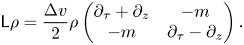
Acting $\it{\boldsymbol{\mathsf{L}}}$ on $\it{\boldsymbol{\varPhi}}$
 leads to a diagonal differential operator on $g$
 in (A5) and gives $\it{\boldsymbol{\mathsf{L}}}\it{\boldsymbol{\varPhi}} =\it{\boldsymbol{\mathsf{0}}}$
 . Finally, using earlier expressions of $\partial _\tau g$
 and $\partial _z g$
 , (2.15) is evaluated to

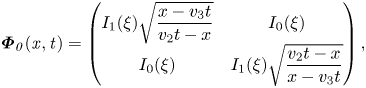
where $\xi (x,t)=(2\gamma _0/\Delta v)\sqrt {(v_2t-x)(x-v_3t)}$ . The kernel $\it{\boldsymbol{\varPhi}} _0$
 is in the interior of the light cone, whose contribution vanishes when the coupling is zero. The $\delta$
 –function terms are on the boundaries of the light cone, which track the wave fronts as the waves advect.
Appendix B. Well-posed boundary conditions
In order for the backscattering problem $v_3<0$ to be well-posed, the boundary conditions need to satisfy constrains. In frequency domain, the constraints $(0, \tilde {l}_3(\omega ))^\mathrm {T} =\tilde {\it{\boldsymbol{\varPsi}} }_0(\omega )\tilde {\boldsymbol {l}}(\omega )$
 are degenerate, which give (2.23) whose inverse is

where $\sigma ={\rm i}\omega$ . To find the relation between boundary conditions in time domain, take inverse Laplace transform $\mathcal {L}^{-1}[\tilde {p}(\sigma )](s)=\int _\mathcal {C} ({{\rm d}\sigma }/{2{\rm \pi} {\rm i}}) \exp(s\sigma )\tilde {p}(\sigma )$
 , where the contour $\mathcal {C}$
 runs from $-{\rm i}\infty$
 to $+{\rm i}\infty$
 on the right-hand side of all poles. First, we need to find the inverse transforms of $\tilde {f}_\pm (\sigma )=\sigma \pm \sqrt {\sigma ^2-1}$
 . Note that $\tilde {f}'_{-}(\sigma )=-\tilde {I}_1(\sigma )$
 . In other words, $\tilde {f}'_{-}(\sigma )=\partial _\sigma \int _0^{+\infty } {\rm d} s \exp(-s\sigma )I_1(s)/s$
 , so $\mathcal {L}[I_1(s)/s](\sigma )=\int {\rm d}\sigma \,\tilde {f}'_{-}(\sigma )=\tilde {f}_{-}(\sigma )+c_{-}$
 . To see that the integration constant $c_-$
 is zero, note that when $\sigma \rightarrow +\infty$
 , Laplace transforms approach zero, so is $\tilde {f}_{-}(\sigma )$
 . Therefore, the inverse transform is
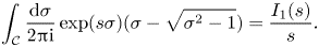
Using the above result and $\mathcal {L}^{-1}[\sigma ](s)= \partial _s\int _{-\infty }^{+\infty } ({{\rm d}\omega }/{2{\rm \pi} })\exp({\rm i}\omega s)=\delta '(s)$ , the inverse Laplace transform of $\tilde {f}_{+}(\sigma )=2\sigma -\tilde {f}_{-}(\sigma )$
 is
is
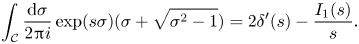
When $s>0$ , the inverse transform of products is $\mathcal {L}^{-1}[\tilde {p}\tilde {q}](s)=\int _0^s {\rm d} s'\,p(s')q(s-s')$
 . Therefore, the inverse Laplace transform of (2.23) is given by (2.24), and the inverse transform of (B1) is

To show that (B4) and (2.24) is an inversion pair, the following identity is needed. Substituting $l_2$ into $l_3$
 , the double integral of $l_3(s-s'-s'')$
 can be simplified by changing the integration variables from $s'$
 and $s''$
 to $\chi =s'+s''$
 and $\eta =s'-s''$
 , where the triangular domain of the double integral ${\rm d} s'\,{\rm d} s''=\frac {1}{2}{\rm d}\eta \,{\rm d}\chi$
 is rotated to $\chi \in [0,s]$
 and $\eta \in [-\chi,\chi ]$
 . The inner $\eta$
 integral is
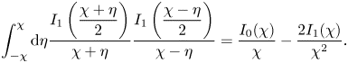
To show the above identity, express $I_1(s)/s$ in terms of its inverse Laplace transform using (B2), where $\frac {1}{2}(\chi \pm \eta )$
 is paired with $\sigma _\pm$
 . Moving the $\sigma _\pm$
 integrals outwards and computing the $\eta$
 integral first leads to $\exp [\chi (\sigma _+ + \sigma _-)/2] \int _{-\chi }^{\chi } {\rm d}\eta \exp [\eta (\sigma _+ - \sigma _-)/2]$ $=2[\exp(\chi \sigma _+)-\exp({\chi \sigma _-})]/(\sigma _+ - \sigma _-)$
 . By the $\sigma _+\leftrightarrow \sigma _-$
 symmetry of the outer integrals, it is sufficient to consider the $\exp(\chi \sigma _+)$
 term, which can be moved outside the $\sigma _-$
 integral. Closing the contour from right in the complex $\sigma _-$
 plane, $\int _\mathcal {C_-} ({{\rm d}\sigma _-}/{2{\rm \pi} {\rm i}}) [\sigma _- - (\sigma _-^2-1)^{1/2}]/(\sigma _+ - \sigma _-)= \frac {1}{2}[\sigma _+ - (\sigma _+^2-1)^{1/2}]$
 , where the factor $\frac {1}{2}$
 comes from the fact that a pole is enclosed only when the contour $\mathcal {C_-}$
 is on the left of $\mathcal {C_+}$
 . To show that the remaining integral $\int _\mathcal {C_+} ({{\rm d}\sigma _+}/{4{\rm \pi} {\rm i}})\exp(\chi \sigma _+) [\sigma _+ - (\sigma _+^2-1)^{1/2}]^2$
 equals to the right-hand side of (B5), compute its Laplace transform $\tilde {F}(\sigma _+)=\int _0^{+\infty } {\rm d}\chi \exp ({-\chi \sigma _+})[I_0(\chi )/\chi -2I_1(\chi )/\chi ^2]$
 . Taking derivatives to remove denominators gives $\tilde {F}''(\sigma _+)=-\tilde {I}'_0(\sigma _+)-2\tilde {I}_1(\sigma _+)$
 , which can be integrated twice to give $\tilde {F}(\sigma _+)=\sigma _+^2-\sigma _+(\sigma _+^2-1)^{1/2}+c_1\sigma _+ + c_2$
 using $\tilde {I}_0$
 and $\tilde {I}_1$
 found before (2.23). The integration constants $c_1=0$
 and $c_2=-\frac {1}{2}$
 are determined using the condition $\tilde {F}(+\infty ) = 0$
 , which gives $\tilde {F}(\sigma _+)=\frac {1}{2}[\sigma _+ - (\sigma _+^2-1)^{1/2}]^2$
 as desired. Finally, substituting (B5) into the $l_3(s-s'-s'')$
 integral partially cancels with the $l_3'(s-s')$
 term after integration by parts, and what remains are the boundary terms $l_3(s)-2l_3(0)I_1(s)/s$
 . The second term vanishes because $l_3(0)=0$
 , which is a consequence of (2.24). We have thus shown that $l_3[l_2]=l_3$
 . Similarly, substituting $l_3$
 into $l_2$
 and using (B5), the converse can also be shown.
Verifying that $l_2$ and $l_3$
 satisfy the constraints in the time domain requires the following identity. For the first constraint $0=\int _0^s {\rm d} s'[I_1(s')l_2(s-s')-\sqrt {|v_3|/v_2}I_0(s')l_3(s-s')]$
 , express $l_3$
 in terms of $l_2$
 using (2.24) and change the double integral of $l_2(s-s'-s'')$
 from $s'$
 and $s''$
 to $\chi =s'+s''$
 and $\eta =s'-s''$
 . The constraint is satisfied because

The proof of this identity is similar to (B5), where $I_0(s)$ and $I_1(s)/s$
 are expressed in terms of their inverse Laplace transforms and the $\eta$
 integral is performed before closing the $\sigma _\pm$
 contours. Finally, for the second constraint $2l_3(s)=\int _0^s {\rm d} s'[\sqrt {v_2/|v_3|}I_0(s')l_2(s-s') -I_1(s')l_3(s-s')]$
 , express $l_2$
 in terms of $l_3$
 using (B4). After integration by part for the $l'_3(s-s')$
 term, which yields a boundary term and an integral that cancels the remaining terms due to (B6), it is easy to see that this constraint is also satisfied.
Appendix C. Properties of kernel functions
To verify that (2.25) satisfies boundary conditions, special values of $M_2$ and $M_3$
 are needed. At the boundary, $\vartheta =0$
 and $M_2(\varphi,0)=\int _0^1{\rm d} r\, I_0(r\varphi )I_1(\varphi (1-r))/(1-r)$
 . The integral recovers (B6) after changing variable to $\varphi '=(2r-1)\varphi$
 , so
, so
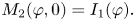
Hence, $D_2(\varphi, 0)=0$ and $\alpha _2(x=0, t)=h_0$
 satisfies the boundary condition. Similarly, changing the integration variable to $\varphi '$
 gives
gives
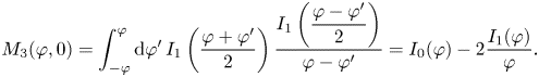
The proof of this identity is similar to (B5) and (B6). Substituting $D_3(\varphi,0)=2I_1(\varphi )/\varphi$ into (2.25) recovers $\alpha _3(x=0,t)=h_3(t)$
 . The other special values are at $\varphi \rightarrow 0$
 . Using $I_1(\varphi )\simeq \varphi /2$
 , $M_2(0,\vartheta )=M_3(0,\vartheta )=0$
 , $D_2(0,\vartheta )=\vartheta$
 and $D_3(0,\vartheta )=1$
 .
.
To verify that (2.25) solves $\it{\boldsymbol{\mathsf{L}}} \boldsymbol {\alpha }=\boldsymbol {0}$ , differential properties of the kernel functions are needed. Using $d_y\int ^{b(y)}_{a(y)} {{\rm d}x}\,f(x,y)=\int ^{b}_{a} {{\rm d}x}\,\partial _yf(x,y) + b'(y)f(b,y) - a'(y)f(a,y)$
 where $a$
 and $b$
 are evaluated at $y$
 , the derivatives $\partial _t\alpha _2$
 and $\partial _x\alpha _2$
 can be easily computed, where the latter involves $\partial _\vartheta D_2(\varphi,\vartheta )$
 . Using the properties of modified Bessel functions,
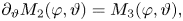
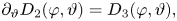
which ensures $(\partial _t+v_2\partial _x+\mu _2)\alpha _2=\gamma _0\alpha _3$ is satisfied by (2.25). To show that $(\partial _t+v_3\partial _x+\mu _3)\alpha _3=\gamma _0\alpha _2$
 is also satisfied, note that $(v_3\partial _x+\mu _3) \exp ({-\mu _2x/v_2})$
 gives a term proportional to $\int _0^{\gamma (t-x/v_2)}{\rm d}\varphi \, D_3(\varphi,\vartheta ) \partial _\varphi \exp ({-\varphi \gamma _a/\gamma _0})$
 , which can be computed using integration by parts. Using the special value $D_3(0,\vartheta )=1$
 and identities

the $\alpha _3$ equation is straightforward to verify. To show the first equality in (C4), use the definitions of $D_2$
 and $D_3$
 before (2.26) and $(2\partial _\varphi -\partial _\vartheta )I_0 = \sqrt {1+2\vartheta /\varphi }I_1$
 . To show the second equality, $(2\partial _\varphi -\partial _\vartheta )M_3(\varphi,\vartheta )$ $= \int _0^1{\rm d} r\{[I'_0(2\partial _\varphi \partial _\vartheta \xi -\partial _\vartheta ^2\xi ) + I''_0(2\partial _\varphi \xi -\partial _\vartheta \xi )\partial _\vartheta \xi ]I_1/(1-r) + 2I'_0I'_1\partial _\vartheta \xi \}$
 , where the argument of $I_0$
 is $\xi =\sqrt {r^2\varphi ^2+2r\varphi \vartheta }$
 and the argument of $I_1$
 is $\varphi (1-r)$
 . Using derivatives of $\xi$
 and the differential equation for $I_0$
 , the two terms in the square bracket combine to $r^2\varphi [(2r-1)\varphi +2\vartheta ]I_0/\xi ^2-2r^2\varphi ^2(r-1)I'_0/\xi ^3$
 . The remaining term is $\int _0^1{\rm d} r\,I'_0I'_1\partial _\vartheta \xi = -\int _0^1{\rm d} r\,(rI'_0/\xi )\partial _r I_1 =\int _0^1{\rm d} r\, I_1\partial _r(rI'_0/\xi )$
 , because the boundary terms are zero. This term equals $\int _0^1{\rm d} r\, I_1[(1-r\varphi \vartheta /\xi ^2)I_0-r^2\varphi ^2I'_0/\xi ^3]$
 . Summing all contributions, the $I'_0$
 terms cancel and $(2\partial _\varphi -\partial _\vartheta )M_3(\varphi,\vartheta ) = \int _0^1{\rm d} r\,cI_0I_1/(1-r)$
 , where $c=r^2\varphi [(2r-1)\varphi +2\vartheta ]/\xi ^2+2(1-r)(1-r\varphi \vartheta /\xi ^2)=1$
 . Using the definition of $M_2$
 in (2.26), the second equality in (C4) is thus proved.
Finally, let us analyse the limit $t\rightarrow +\infty$ for two special cases. First, at the boundary, $\alpha _3(x=0,t)=h_0\sqrt {v_2/|v_3|} \varDelta (\gamma t, \varsigma )$
 , where $\varDelta (s, \varsigma )=\int _0^{s} {\rm d} s'\exp ({-\varsigma s'}) I_1(s')/s'$
 and $\varsigma =\gamma _a/\gamma _0$
 measures damping relative to growth. When $\gamma _0>\gamma _a$
 is above the absolute instability threshold, the integral diverges and $\varDelta (+\infty, \varsigma <1)=+\infty$
 . On the other hand, when $\gamma _0\le \gamma _a$
 , the integral converges and is given by (B2) as $\varDelta (+\infty, \varsigma \ge 1)=\varsigma -\sqrt {\varsigma ^2-1}$
 . At the threshold $\gamma _0=\gamma _a$
 , using property of modified Bessel function (DLMF 2022, (10.43.8)), the special value is $\varDelta (s, \varsigma =1)=1-\exp(-s)[I_0(s)+I_1(s)]\simeq 1-\sqrt {2/{\rm \pi} s}$
 , so the steady state is approached only at an algebraic rate. Second, at zero plasma wave velocity $v_3=0$
 , the solutions are given by (2.27). When $t\rightarrow +\infty$
 , the integrals are evaluated using property of modified Bessel function (DLMF 2022, (10.43.24)) and $I_{1/2}(x)=\sqrt {2/{\rm \pi} x}\sinh x$
 . To see how fast the solutions approach steady states, consider the residual $\mathcal {R}=\int _\psi ^{+\infty } {\rm d}\xi \exp ({-\nu \xi ^2})I_1(\xi )$
 . The residual diminishes exponentially as $\exp ({-\nu \psi ^2})=\exp ({-\mu _3t_r})$
 when $\psi \gg \xi _*$
 , where $t_r=t-x/v_2$
 is the retarded time. The threshold $\xi _*$
 maximises the integrand of $\mathcal {R}$
 and is the unique root of $I_0(\xi _*)/I_1(\xi _*)=1/\xi _*+2\nu \xi _*$
 . When $\nu \gg 1$
 , namely when the spatial gain is small, $\xi _*\simeq 1/\sqrt {2\nu }$
 , so the growth saturates when $t_r\gg 1/\mu _3$
 . On the other hand, when $\nu \ll 1$
 , namely when the spatial gain is large, $\xi _*\simeq 1/2\nu$
 , so the growth saturates when $t_r\gg \gamma _0^2x/\mu _3^2v_2$
 . To give a better approximation of $\mathcal {R}$
 when $\nu \ll 1$
 , note that $\xi >\psi \gg \xi _*\gg 1$
 so $I_1(\xi )\simeq \exp(\xi) /\sqrt {2{\rm \pi} \xi }$
 . Changing the integration variable gives $\mathcal {R}\simeq ({1}/{2\sqrt {2{\rm \pi} }}) \exp(1/4\nu)\int _{\zeta _0}^{+\infty } {\rm d}\zeta \,\exp({-\zeta })[\zeta (\frac {1}{2}+\sqrt {\nu \zeta })]^{-1/2}$
 , where $\zeta _0=\nu (\psi -1/2\nu )^2=\mu _3t_r-\sqrt {\mu _3t_r/\nu }+1/4\nu$
 . When $\nu \zeta _0\gg \frac {1}{4}$
 , which is equivalent to $t_r\gg 4\gamma _0^2x/\mu _3^2v_2$
 , the $\frac {1}{2}$
 term is negligible, and the integral is evaluated to $\mathcal {R}\simeq ({1}/{2\sqrt {2{\rm \pi} }}) \exp(1/4\nu) \nu ^{-1/4}\varGamma (\frac {1}{4}, \zeta _0)$
 using the incomplete gamma function $\varGamma (n,z)=\int _z^{+\infty } {\rm d}\zeta \,\zeta ^{n-1}\exp(-\zeta)\simeq z^{n-1}\exp(-z)$
 .
.


 Open access