


1. Introduction
The vortex flows around an inclined hemisphere–cylinder body have been studied for decades as a canonical model in the aerospace and submarine industries, as well as the academic community. Various vortex structures have been identified over a hemisphere–cylinder body. The leeward vortices are strongest and contribute to most of the aerodynamic forces on the body, being characterized by a pair of counter-rotating vortices that is formed by curving of shear layers separated from both sides of the body. In the rear end, rear-end vortices exist, commonly in a shedding form. In some cases, a separation bubble and horn vortices with small scale can be found near a nose, depending on the angles of attack (AOAs) and Reynolds number ( $Re$) based on the diameter of the cylinder (Hsieh & Wang Reference Hsieh and Wang1996; Le Clainche et al. Reference Le Clainche, Rodríguez, Theofilis and Soria2016).
Previous studies have shown that low-frequency unsteadiness exists for the leeward vortices around a hemisphere–cylinder body in numerical simulations and experiments. In early studies, Hoang, Rediniotis & Telionis (Reference Hoang, Rediniotis and Telionis1999) measured fluctuations of the leeward vortices over a hemisphere–cylinder body at AOAs of  $10^{\circ }$– $90^{\circ }$ and $Re=22\,000$ using two hot-wire probes, and discovered lower frequency components than those of Kármán vortex shedding. Subsequently, Sirangu & Ng (Reference Sirangu and Ng2012) used a smoke visualization to show that the vortices around the afterbody of a hemisphere–cylinder body can change their orientations over time, thus providing further evidence of vortex fluctuations. Le Clainche et al. (Reference Le Clainche, Li, Theofilis and Soria2015) conducted a numerical simulation on a hemisphere–cylinder body at ${\rm AOA} = 20^{\circ }$, and $Re=350$ and 1000, in which symmetric modes were found for an oscillatory horn/leeward vortex system.
Ma & Yin (Reference Ma and Yin2018) reported a vortex oscillation phenomenon around a hemisphere–cylinder body using a large-eddy simulation where the Reynolds number is identical to that used by Hoang et al. (Reference Hoang, Rediniotis and Telionis1999). The results reveal that the antisymmetric wavy oscillations of leeward-vortex pairs exist over a forebody at AOAs of  $10^\circ$– $80^\circ$ in addition to vortex shedding at an afterbody. The alternate vortex oscillations correspond to the most energetic modes, and are responsible for the fluctuating sectional side forces on the forebody, which are greater than those from vortex shedding at the afterbody. Jiang & Ma (Reference Jiang and Ma2019) further performed particle image velocimetry experiments over a hemisphere–cylinder body at a fineness ratio of 8, in which the vortex shedding almost disappears due to the shorter afterbody, whereas the alternate vortex oscillation still exists even without vortex shedding, implying that the oscillations arise from intrinsic instabilities of the leeward vortex pair. The estimated streamwise wavenumbers of the wavy vortex cores indicate that the vortex oscillations seem to come from long-wave instabilities. Recent studies further confirmed the occurrence of low-frequency vortex oscillations in experiments (Yuan & Yarusevych Reference Yuan and Yarusevych2020) and simulations (Ijaz & Ma Reference Ijaz and Ma2022). In addition, Strandenes et al. (Reference Strandenes, Jiang, Pettersen and Andersson2019) also numerically reported a similar vortex oscillation phenomenon around an inclined prorate spheroid.
Nevertheless, the underlying mechanism on the vortex oscillations is still unclear. From phenomena, they seem different from the existing unsteady vortex motions arising from flow instabilities, such as vortex shedding past blunt bodies (Pier Reference Pier2008; Bohorquez et al. Reference Bohorquez, Sanmiguel-Rojas, Sevilla, Jiménez-González and Martínez-Bazán2011), vortex wandering around a wing tip (Edstrand et al. Reference Edstrand, Davis, Schmid, Taira and Cattafesta2016) or over delta wings (Ma, Wang & Gursul Reference Ma, Wang and Gursul2017). Their origin should be closer to Crow-type long-wave instabilities of a parallel vortex pair (Donnadieu et al. Reference Donnadieu, Ortiz, Chomaz and Billant2009; Leweke, Le Dizes & Williamson Reference Leweke, Le Dizes and Williamson2016), because the leeward vortices around a hemisphere cylinder are a pair of streamwise vortices. However, the long-wave instabilities exhibit symmetric modes and no self-sustained oscillation will be formed. Therefore, local stability analysis based on parallel vortex pairs is insufficient for exploring the mechanism of the vortex oscillation. In this study, we appeal to the global stability analysis of a fully three-dimensional base flow, also called a ‘Tri-Global’ analysis by Theofilis (Reference Theofilis2011), to examine this unsteady vortex phenomenon. We first reproduce the vortex oscillation via numerical simulations, and then obtain the base flow and analyse the global stability.
2. Methodology
The numerical simulations are based on the incompressible Navier–Stokes equations, and the global stability analysis uses the linearized Navier–Stokes equations. These equations are solved using an open-source spectral/hp element code Nektar++ (Cantwell et al. Reference Cantwell2015), which has been extensively verified and validated, and applied to global stability analysis in separated flow and vortices (He et al. Reference He, Gioria, Pérez and Theofilis2017). Details on the numerical methods are presented as follows.
2.1. Numerical grids and simulation methods
The geometric model, computational domain and grids are illustrated in figure 1. The model is a circular cylinder with a hemisphere cap and the ratio of its total length to diameter is 8. The domain is axially symmetric around the model with a C-O topology, and extends 15 times the diameter of the model upstream and radially, 42.5 times the diameter downstream. The origin of the coordinate ( $x,y,z$) is located at the rear end of the hemisphere cap. No-slip boundary conditions are imposed on the wall of the model; the free stream velocity conditions are applied on the inlet and side surfaces of the domain; a high-order outflow condition is imposed on the outlet to avoid the reflection of perturbations downstream (Dong, Karniadakis & Chryssostomidis Reference Dong, Karniadakis and Chryssostomidis2014; Cantwell et al. Reference Cantwell2015).

Figure 1. Flow configuration around a hemisphere–cylinder body ( $D$ is diameter of cylinder): (a) computational domain; (b) hexahedral grids.
The AOA is fixed at  $30^\circ$ in simulations, which is a typical AOA for the vortex oscillation in terms of previous studies (Ma & Yin Reference Ma and Yin2018; Jiang & Ma Reference Jiang and Ma2019). The Reynolds number based on the diameter of the cylinder remained as 3000. According to the experimental results in a range of $Re=1000$–7000 (Jiang & Ma Reference Jiang and Ma2019), the vortex oscillations occur and gradually grow in amplitude with increasing $Re$. Herein the critical Reynolds number $Re_c$ for the onset of vortex oscillations has been determined through numerical simulations at various Reynolds numbers where the corresponding side force is chosen as an indicator to monitor the occurrence of the oscillations, as shown in figure 2. We will show in § 3 that the local instability region triggering the vortex oscillation is located immediately behind the head of the cylinder, so the vortex oscillations can induce the side force if they occur. The side force coefficients manifest irregular fluctuations with minor amplitude at $Re\leq 2650$, and transition to regular oscillations at $Re\geq 2700$. Therefore, the critical Reynolds number $Re_c$ is between 2650 and 2700. The small parameter $\varepsilon =1/Re_c-1/Re$ is commonly employed to measure the proximity of the current $Re$ to the critical $Re_c$ (Sipp & Lebedev Reference Sipp and Lebedev2007). The parameter $\varepsilon$ cannot be too large, otherwise the base flow is intractable to solve. However, if the difference between $Re$ and $Re_c$ is too small, the flow evolution initialized from a base flow will take a long time to reach a saturated state, which is unfavourable for observing growth of perturbation by numerical simulations. Herein the $Re=3000$ is chosen as the flow condition where the parameter $\varepsilon$ is far less than 1.

Figure 2. Variation of side-force coefficients with  $Re$.
$Re$.
The computational domain is discretized into 9440 grid cells, created by an open-source code GMSH (Geuzaine & Remacle Reference Geuzaine and Remacle2009). Hexahedral grids are used to capture viscous layers and flow separation near a wall. The second-order curvilinear grids are created on the wall to better describe the geometry of the model. For formal computation, the solution in one cell is expanded by an eighth-order polynomial ( $P=8$) that corresponds to a ninth-order spatial precision. The second-order implicit–explicit scheme is employed for time integration. The non-dimensional time step is 0.001, which is mainly limited by the Courant–Friedrichs–Lewy condition in the current case, and much smaller than the physical time scale in flows. The high-order spectral element method is sensitive to the spatial resolution, so spectral vanishing viscosity (SVV) (Kirby & Sherwin Reference Kirby and Sherwin2006) is added in simulations to improve the stability of computation. The SVV filters out high wavenumber perturbative waves smaller than the grid scale, but does not degrade the exponential convergence of the spectral element method. For resolved flow solutions, the SVV only damps out the high-frequency numerical waves, but has no effect on physical fluctuations, which has been theoretically analysed and validated with typical flow examples (Xu & Pasquetti Reference Xu and Pasquetti2004; Kirby & Sherwin Reference Kirby and Sherwin2006). For under-resolved solutions, the SVV can filter out physical fluctuations smaller than the grid scale, and can therefore be regarded as a subgrid model for implicit large-eddy simulation. For our case of $Re=3000$, most of the flow field is laminar, but we cannot indeed rule out the possibility of transition or turbulence occurring somewhere downstream. For a high-order $p$-type spectral element method, the current grid number approximately equals $6.9\times 10^6$ nodal points based on the order of the polynomials and discretized cells. The grid resolution will be validated by means of grid convergence testing in the following.
2.2. Global linear stability analysis
We compute the steady base flow around a hemisphere–cylinder body using the selective frequency damping (SFD) method (Åkervik et al. Reference Åkervik, Brandt, Henningson, Hœpffner, Marxen and Schlatter2006). In this algorithm, a temporal low-pass filtering process is imposed to flow variables with time stepping of the numerical solution, gradually filtering out unstable waves in flow fields, thus constraining the Navier–Stokes equations to converge towards a steady-state solution. The filter coefficients need to be chosen carefully to damp out the lowest frequency unstable modes, and the information of frequencies from numerical simulations can help with the choice. The numerical set-up in SFD is the same as the numerical simulations.
Around the base flow, the Navier–Stokes equations are linearized, and the linearized operator is denoted by a matrix  $\boldsymbol{\mathsf{A}}$. The corresponding global modes can be represented by ${\phi _j}(x,y,z)\,{\rm e}^{{\lambda }_j t},\ j=1,\ldots,m$, where $\phi _j$ and $\lambda _j$ denote eigenmodes and eigenvalues. The real parts and imaginary of $\lambda _j$ give the temporal growth rates and circular frequencies, respectively. Matrix $\boldsymbol{\mathsf{A}}$ is commonly very large (here ${\sim }10^7\times 10^7$), and solving it using the matrix methods is prohibitive. Therefore, herein the iterative approach based on a time-stepping numerical simulation is employed to obtain the global modes. If let $\boldsymbol{\mathsf{B}}={\rm e}^{\boldsymbol{\mathsf{At}}}$, the linear evolution of a perturbation can be expressed as $\boldsymbol {u}'(\boldsymbol {x},t)=\boldsymbol{\mathsf{B}}\boldsymbol {u}'(\boldsymbol {x},0)$ where $\boldsymbol {u}'(\boldsymbol {x},0)$ is an initial perturbation field containing information of the modes to be solved. The eigenmodes and eigenvalues of matrix $\boldsymbol{\mathsf{A}}$ can be recovered through matrix $\boldsymbol{\mathsf{B}}$. The large matrix $\boldsymbol{\mathsf{B}}$ is projected into a smaller size Krylov subspace, so significantly reducing the cost of computation and storage. The Krylov subspace is constructed by snapshots taken from the linearized flow fields. The choice of the time interval ${\Delta }t$ between snapshots needs to satisfy the Nyquist sampling criterion in terms of characteristic time scales in flow fields, and meanwhile, it cannot be too small to distinguish the Krylov vectors, thus deteriorating convergence of iteration. Herein ${\Delta }t$ is set as 0.5 and the dimension of Krylov subspace $m$ is 10. The low-dimensional space is computed by a modified Arnoldi iteration algorithm, which is an equivalent of the implicitly restarted Arnoldi method (Cantwell et al. Reference Cantwell2015).
2.3. Grid convergence testing
For high-order spectral element methods, grid convergence is typically tested by  $p$-type refinement, which increases or decreases the orders of polynomials (Blackburn, Barkley & Sherwin Reference Blackburn, Barkley and Sherwin2008; Mao, Sherwin & Blackburn Reference Mao, Sherwin and Blackburn2012; He et al. Reference He, Gioria, Pérez and Theofilis2017). By this means, the precision of spatial formats will also be changed in addition to grid refinement or coarseness. The $p$-type refinement directly adjusts the order of the polynomial expansions, not requiring remeshing, so it is more convenient. We validated the grid independence of numerical simulations and eigenmodes by altering the polynomial orders $P$ from 7 to 9. The equivalent grid quantities are proportional to the cube of the order $p+1$. The grid quantities of the eighth- and ninth-order expansions are 1.4 and 2.0 times the one of the seventh-order expansion. The results are listed in table 1. In numerical simulations, the time-averaged axial and normal forces, as well as frequencies of the side force are selected to quantify the grid effects on the averaged and time-dependent flow fields. All quantities are non-dimensional with the free stream velocity, diameter and cross-section area of the cylinder as characteristic quantities. The results show that these quantities have a minor variation as the order of polynomials $P$ varies from 7 to 9, particularly for $P=8$ to 9. Effects of time steps are also tested by doubling the original time step 0.001 to 0.002, and the maximum deviation comes from the axial force coefficient, but only 0.9 %. The eighth order of polynomials ( $P=8$) and time step 0.001 are eventually chosen for formal computations of unsteady simulations and steady base flow, as a balance between accuracy and efficiency. The base flows are physically smoother than the unsteady flow fields, so have less requirement for grid resolution. The effects of polynomial orders on eigenmodes in stability analysis are also illustrated in table 1, in which the growth rate is the real part of the eigenvalue and the frequency $St=f\kern 0.06em D/U_{\infty }$ is the imaginary part of the eigenvalue divided by 2 ${\rm \pi}$. Both of them are non-dimensional. The mode with the lowest growth rate and lowest frequency is presented, which is the mode of most interest in the study. It is found that the growth rate with $P=8$ has a difference of 6 % with respect to $P=9$, and $St$ has a 2 % difference. Therefore, we believe that the eighth-order polynomials are suitable to solve the eigenmodes in our cases, and the minor deviations will have no substantial effects on our understanding of the mechanism of vortex oscillation that is the main purpose of the study.
Table 1. Grid convergence testing in numerical simulations and stability analysis.

3. Results and discussion
3.1. Observations from numerical simulations
The vortex oscillations around a hemisphere–cylinder body are numerically reproduced at an AOA of  $30^{\circ }$ and $Re=3000$. The simulation starts from a base flow (see below) to observe the evolution process of the flow field, from a symmetric state to an antisymmetric oscillatory state. Three-dimensional instantaneous vortex structures in saturated states are illustrated in figure 3, in which the vortex structures are identified by the $\lambda _2$ criterion (Jeong & Hussain Reference Jeong and Hussain1995) at a level of $-0.15$, coloured by the $x$-component vorticity. The vortex oscillations manifest antisymmetric motion of the leeward-vortex pair, including alternate up-and-down oscillation and in-phase side-to-side motion. The three-dimensional vortex axes exhibit wavy patterns, which belong to long waves in terms of ratios of the wavelength with respect to the size of vortex cores or separation between two cores, as revealed in previous studies (Jiang & Ma Reference Jiang and Ma2019). The two instantaneous states exhibit an approximately opposite phase of oscillation. Figure 4 depicts the instantaneous sectional flow fields at $x/D=6$, which more clearly shows the alternate up–down oscillation of the vortex pair. The saturated oscillation phase is computed for 17 cycles, on which 240 snapshots in a time interval of 0.5 are extracted for obtaining the time-averaged flow, as displayed in figure 5 with the $\lambda _2$ criterion. Since the time-averaged flow is an average of the oscillatory vortices, the vortex surfaces identified do not represent real concentrated vortices, particularly for the downstream portion of the vortex pair where the vortices have greater amplitude of oscillation. The vortex surfaces downstream of the cylinder need to be visualized with small $\lambda _2$ values.

Figure 3. Two instantaneous snapshots of vortex oscillations around a hemisphere–cylinder body, identified by  $\lambda _2$ method (top view).

Figure 4. Oscillation of the leeward-vortex pair at section  $x/D=6$: (a) $t^*=t_0$; (b) $t^*=t_0+2$; (c) $t^*=t_0+4$.

Figure 5. Time-averaged flow around a hemisphere–cylinder body, identified by the  $\lambda _2$ method: (a) side view; (b) top view.
The oscillatory behaviours of the vortices can be quantitatively described in terms of time histories of the side force induced by vortex oscillations, as shown in figure 6(a). Since the flow fields are initialized from a base flow with a minor stochastic perturbation ( $10^{-5}$ in magnitude), the side force approaches zero in amplitude at the initial stage, and then the amplitude gradually grows in time with the flow losing stability until a saturated oscillatory state is reached, where the side force fluctuates with approximately constant amplitude. The frequency spectrum for the steady oscillation is computed by the fast Fourier transform (FFT) and presented in figure 6(b), where an isolated frequency peak is visible, indicating that the vortex oscillations contributing most to unsteady aerodynamic loads have a good single–frequency periodicity. The non-dimensional frequency $St$ characterized by the free stream velocity and the diameter of the cylinder is 0.109, which is consistent with $St=0.11$ obtained in previous studies (Ma & Yin Reference Ma and Yin2018; Jiang & Ma Reference Jiang and Ma2019). The normal force coefficients are shown in figure 7(a), which can detect symmetric modes of the vortex pair, corresponding to in-phase up–down oscillations. The normal force coefficients of the time-averaged and base flows are also shown where the latter is much lower than the former. The frequency spectrum for the saturated oscillation of the normal force is shown in figure 7(b), the peak frequency $St=0.213$ is close to half of the side force one.

Figure 6. Fluctuation of the total side force coefficient of the hemisphere–cylinder body: (a) time history; (b) frequency spectrum.

Figure 7. Fluctuation of the total normal force coefficient of the hemisphere–cylinder body: (a) time history; (b) frequency spectrum.
The dynamic mode decomposition (DMD) (Rowley et al. Reference Rowley, Mezić, Bagheri, Schlatter and Henningson2009; Schmid Reference Schmid2010) is also carried out for the saturated stage to find the dominant frequencies and oscillatory modes. Herein we use the companion matrix to implement the decomposition and the averaged flow field has been removed from the series of snapshots. We have tested the effects of the snapshot number on the results of DMD with 121, 160, 200 and 240 snapshots. As the snapshots exceed 200, the frequencies of the modes exhibit good regularity. For the 200 and 240 snapshots, the frequency difference of each mode is limited below 1.8 %. The results of the 240 snapshots with a sampling interval of 0.5 are presented in figure 8. Figure 8(a) shows the frequency spectrum of DMD, where the frequency of the most energetic mode (Mode 1) is 0.112 that is in good agreement with the preceding FFT frequency of the side force ( $St=0.109$) in figure 6(b), and the frequency of Mode 2 is 0.216, which is consistent with the frequency of the normal force ( $St=0.213$) in figure 7(b). Modes 1 and 2 are plotted in figure 8(b,c) with top and side views, visualized by isocontours of the $y$-component velocity $v'/U_{\infty }$. The distribution of $v'/U_{\infty }$ for Mode 1 is symmetric, indicating the mode is antisymmetric; similarly, Mode 2 is symmetric (Bagheri et al. Reference Bagheri, Schlatter, Schmid and Henningson2009). Mode 1 corresponds to the antisymmetric oscillation of the vortex pair, as shown in figures 3 and 4. Mode 2 corresponds to the in-phase up-down oscillation of the vortex pair, which has also been reported in previous studies (Ma & Yin Reference Ma and Yin2018; Jiang & Ma Reference Jiang and Ma2019). The Modes 3 and 5 in figure 8(a) are antisymmetric and harmonic frequencies of Mode 1; Mode 4 is symmetric and a harmonic frequency of Mode 2. Modes 3 and 4 are depicted in figure 8(d,e). All these modes start from immediately behind the head of the cylinder and occupy the entire region over the body and convect downstream. The existence of harmonic frequencies indicates that vortex oscillations are not single-frequency oscillations, but not representing new flow phenomena. Nevertheless, the modes higher than Mode 2 have much lower energy, and contribute little to the aerodynamic forces. Therefore, no high-frequency components are visible on the frequency spectra of side and normal forces in figures 6(b) and 7(b).

Figure 8. Frequency spectrum and modes of DMD: (a) frequency spectrum; (b) Mode 1 with  $St=0.115$; (c) Mode 2 with $St=0.216$; (d) Mode 3 with $St=0.327$; (e) Mode 4 with $St=0.431$.
3.2. Base flow and global modes
The base flow for stability analysis obtained by SFD is illustrated in figure 9, visualized by the  $\lambda _2$ criterion and coloured by the $x$-component vorticity. The steady base flow is characterized by a pair of counter-rotating vortices over the leeward side of the hemisphere–cylinder body. The formation of the vortex pair originates from curving of shear layers separated from both sides of the body. The shear layers continuously feed vorticity into the vortex cores along the separation lines, so the circulation and size of vortices gradually grow along the vortex axes until the rear end of the body. For the vortex portion located above the model, the vortex axes are approximately aligned with the body axis of the model. Beyond the rear end, the vortex pair turns into free vortices and no more vorticity is fed, and the vortices slowly decay due to viscosity dissipation as they travel downstream, and the vortex axes deflect up towards the free stream direction. Therefore, the leeward vortices reach the maximum strength near the rear end of the body. Due to the presence of the trailing edge of the cylinder, the shear layers separated from both sides of the cylinder have a discontinuity at the trailing edge, so the vortex pair appears not to be so smooth. Compared with the time-averaged flow in figure 5, the base flow has a slender vortex pair as expected. The sectional vorticity and streamlines of the vortex pair are depicted in figure 10 with two sections on the body ( $x/D=5$) and downstream of the body ( $x/D=15$). Figure 10(a) clearly demonstrates that the leeward vortices are wrapped by the separated shear layers, and figure 10(b) shows that the free vortex pair downstream locally resembles a parallel vortex pair where the streamline around a vortex is not circular, but tends to be elliptical, due to interactions of the strain rate of the opposite vortex. The vortex interactions are major mechanisms of instabilities of parallel vortex pairs (Donnadieu et al. Reference Donnadieu, Ortiz, Chomaz and Billant2009; Leweke et al. Reference Leweke, Le Dizes and Williamson2016).

Figure 9. Base flow around a hemisphere–cylinder body, identified by the  $\lambda _2$ method: (a) perspective view; (b) top view.

Figure 10. Sectional plots of the base flow at various sections: (a)  $x/D=5$; (b) $x/D=15$.
The global spectrum with the four unstable eigenvalues is shown in figure 11(a) where the horizontal and vertical axes represent non-dimensional imaginary and real parts of the eigenvalues. The imaginary part denotes the circular frequency, which is written as Strouhal number  $St$ here to make a comparison with the frequencies of numerical simulations. The real part represents the growth rate of perturbation. Two symmetric modes ( $S_1$ and $S_2$) and two antisymmetric modes ( $A_1$ and $A_2$) are obtained as converged solutions of the Arnoldi iteration. The modes are labelled and sorted by their symmetry and growth rate. The symmetric Mode $S_1$ has the highest growth rate of 1.190 and frequency $St$ of 0.412. The growth rate of Mode $A_1$ is 0.817, slightly lower than Mode $S_1$, but the frequency $St$ (0.416) is similar. Mode $S_2$ has a growth rate of 0.672 and frequency $St$ of 0.220. Mode $A_2$ exhibits the lowest growth rate (0.285) and frequency $St$ (0.105). To validate the correctness of the growth rate, we use each mode as an initial perturbation to trigger the base flow and observe the energy growth of the perturbation over time when evolved under the linearized Navier–Stokes equations. In this case, a symmetric perturbation will trigger the growth of a global mode with the same symmetry and vice versa (Bagheri et al. Reference Bagheri, Schlatter, Schmid and Henningson2009). Four curves of energy growth are illustrated in figure 11(b), and they all exhibit good exponential growth where their slopes are twice the growth rates of the unstable modes. Note that the iterative methods with the time stepper for stability analysis theoretically can compute the most unstable first few modes, but the achievable modes also depend on initial perturbations. The Arnoldi iteration based on a fully three-dimensional base flow is extremely time consuming, particularly for relatively complex geometries, like our case. We believe that the unstable modes of most interest have been obtained due to a long iteration time with various initial values. Higher frequency modes corresponding to the saturation state with low energy may exist, but they are already difficult to determine.

Figure 11. Four unstable modes of the base flow around a hemisphere–cylinder body: (a) eigenvalues diagram of unstable modes, herein  $\lambda _i$ is the imaginary part of the eigenvalue, and $\lambda _r$ the real part; (b) energy growth caused by each of four modes as an initial perturbation.
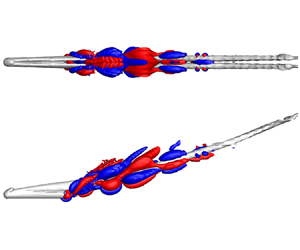
To better compare with the DMD modes, the global linear modes are presented below according to frequency magnitude, instead of growth rate. The antisymmetric Mode  $A_2$ corresponds to Mode 1 of DMD where the vortex pair exhibits the alternate oscillation, as shown in figure 12, which is the mode of most interest to us. The frequency $St$ (0.105) in Mode $A_2$ closely matches the frequencies of the alternate oscillation of vortices (0.109 in side force and 0.112 in Mode 1 of DMD). The frequencies of global linear modes are not necessarily the same as the ones of saturated oscillations, and in many cases, they are different. This is explained by the difference between the base flow and time-averaged flow (Barkley Reference Barkley2006; Sipp & Lebedev Reference Sipp and Lebedev2007). In the present case, however, both frequencies have a good agreement, which is most likely attributed to the unstable regime being close to the critical Reynolds number. The mode frequencies can be exploited for predicting frequencies of vortex oscillations, although this is not our main purpose in this study. It should be noted that the global linear mode in figure 12(a) appears different from Mode 1 of DMD in figure 8(b), where this Mode $A_2$ only occupies the downstream region of the cylinder, but the DMD mode almost extends to the head of the cylinder. However, the difference in appearance is just a display issue. If we reduce the values of velocity $v'/U_{\infty }$, as shown in figure 12(b), the Mode $A_2$ also starts from the region immediately behind the head of the cylinder which is the most front position that the mode can reach. Lowering $v'/U_{\infty }$ further cannot make the mode extend forward until the noise from numerical errors occurs. The difficulty in displaying the global linear modes is that the maximum magnitude of the modes downstream is much larger than other regions, which is very different from the DMD modes. The theoretical basis of the DMD is the Koopman operator, which makes a linear projection of nonlinear flow fields, so the DMD modes remain characteristics of nonlinear modes in appearance. The previous studies on linear and nonlinear stability analyses have clarified the difference between the global linear and nonlinear modes (Huerre & Monkewitz Reference Huerre and Monkewitz1990; Chomaz Reference Chomaz2005). For globally unstable flows, local absolute and convective instability regions are embedded in the flow fields; in our case, the regions include the portion of the vortex pair located over the cylinder and the near wakes behind the trailing edge. The flows are locally stable upstream and downstream of this instability region. The magnitude of the nonlinear modes in the entire local instability region has a small difference due to the saturation of amplitude. By contrast, the global linear modes reach the maximum at the downstream boundary separating the local convective and stable regions due to the perturbation growth along the streamwise direction; meanwhile, their magnitude downstream is much larger than other regions. Therefore, the global instabilities responsible for the vortex oscillations originate upstream, immediately behind the head of the cylinder where a local absolute instability region, also called ‘wavemaker’, exists and triggers the global instability. However, since the maximum value of Mode $A_2$ is located downstream of the rear end, the vortex pair will first produce visible oscillations near the rear end when it loses stability from a base flow, which has been observed in numerical simulations. The differences between the DMD and global linear modes also can be found in the global stability of a jet in cross-flow based on a fully three-dimensional base flow (Bagheri et al. Reference Bagheri, Schlatter, Schmid and Henningson2009; Rowley et al. Reference Rowley, Mezić, Bagheri, Schlatter and Henningson2009). Bagheri et al. (Reference Bagheri, Schlatter, Schmid and Henningson2009) have explained the discrepancies of their global linear modes with numerical simulations, which is similar to our case. Although the local absolute instability region starts upstream, the portions of the vortex pair located over the cylinder and at near-wake region are also locally unstable, absolutely or convectively.

Figure 12. Low-frequency antisymmetric mode ( $A_2$) with growth rate 0.285 and $St$ 0.105: (a) $v'/U_{\infty }=\pm 10^{-5}$ (top and side views); (b) $v'/U_{\infty }=\pm 10^{-8}$ (top view).
The symmetric Mode  $S_2$ with $St=0.220$ is plotted in figure 13, in which figure 13(a) shows the larger magnitude of $v'/U_{\infty }$ and base flow (grey), and the visualization with a lower magnitude of $v'/U_{\infty }$ is depicted in figure 13(b). Mode $S_2$ corresponds to the in-phase oscillations of vortices with the frequencies $St=0.213$ in normal force and 0.216 in Mode 2 of DMD. The Mode $S_2$ with a wave packet form also starts near the head of the cylinder and convects downstream, but its larger value is concentrated near the rear end.

Figure 13. Low-frequency symmetric mode ( $S_2$) with growth rate 0.672 and $St$ 0.220: (a) $v'/U_{\infty }=\pm 10^{-5}$ (top and side views); (b) $v'/U_{\infty }=\pm 10^{-9}$ (top view).
The symmetric Mode  $S_1$ and antisymmetric Mode $A_1$ are shown in figures 14 and 15, and the base flow (grey) is also added as a reference in figures 14(a) and 15(a), and lower magnitude of $v'/U_{\infty }$ for displaying the modes are illustrated in figures 14(b) and 15(b). Mode $S_1$ and $A_1$ still extend downstream from the head of the cylinder, but have greater magnitude of $v'/U_{\infty }$ downstream of the rear end and under the vortex pair. Mode $S_1$ with $St=0.412$ corresponds to the DMD Mode 4 with $St=0.431$, and they are all symmetric and the frequencies are well matched. Mode $A_1$ with $St=0.416$ corresponds to the DMD Mode 3 with $St=0.327$, and they are all antisymmetric, but the frequencies have a discrepancy. We attribute the discrepancy to distortion of the time-averaged flow (Barkley Reference Barkley2006; Sipp & Lebedev Reference Sipp and Lebedev2007), in which the base-flow-based linear modes do not necessarily have the same frequencies as the saturated modes. However, why other modes match well and only this mode has deviation is still unclear.

Figure 14. High-frequency symmetric mode ( $S_1$) with growth rate 1.190 and $St$ 0.412: (a) $v'/U_{\infty }=\pm 10^{-5}$ (top and side views); (b) $v'/U_{\infty }=\pm 10^{-9}$ (top view).

Figure 15. High-frequency antisymmetric mode ( $A_1$) with growth rate 0.817 and $St$ 0.416: (a) $v'/U_{\infty }=\pm 10^{-5}$ (top and side views); (b) $v'/U_{\infty }=\pm 10^{-9}$ (top view).
4. Conclusion
The underlying mechanism responsible for the vortex oscillation around a hemisphere–cylinder body is investigated using numerical simulations and global stability analysis. The fully three-dimensional base flow is obtained through a SFD method, which exhibits a pair of steady leeward vortex wrapped by shear layers separated from both sides of the body and turns into free vortex pair downstream of the body. The four unstable modes are obtained using a modified Arnoldi iteration, among which the antisymmetric mode with a Strouhal number of 0.105 is discovered to correspond to the alternate oscillation of the vortex pair, and the symmetric mode with a Strouhal number of 0.220 corresponds to the in-phase vortex oscillation. Their frequencies have a good agreement with the DMD modes. The global linear modes start from the region immediately behind the head of the cylinder and propagate downstream, and reach the maximum downstream of the rear end of the cylinder. The other two unstable modes with higher frequencies, one antisymmetric and one symmetric, are harmonic frequencies of the above two modes. This finding conclusively verifies that the vortex oscillations over a hemisphere–cylinder body originate from a global flow instability.
Funding
The project was supported by the National Natural Science Foundation of China under grant nos 11672021 and 12072015.
Declaration of interests
The authors report no conflict of interest.


