


1. Introduction
Multiscale coherent motions have been discovered in high-Reynolds-number wall-bounded turbulence. Among these motions, large-scale and very-large-scale motions (LSMs and VLSMs, respectively), whose streamwise scale reaches more than 2–3 $\delta$ (where $\delta$ is the outer length scale, i.e. boundary layer thickness, pipe radius and channel half-height), are important and dominant features in wall-bounded turbulence (Kovasznay, Kibens & Blackwelder Reference Kovasznay, Kibens and Blackwelder1970; Brown & Thomas Reference Brown and Thomas1977; Robinson Reference Robinson1991; Kim & Adrian Reference Kim and Adrian1999; Balakumar & Adrian Reference Balakumar and Adrian2007; Marusic et al. Reference Marusic, McKeon, Monkewitz, Nagib, Smits and Sreenivasan2010). This kind of large-scale coherent motion not only exhibits an oblique angle from the wall in the streamwise direction (i.e. the structure inclination angle) morphologically but also has a significant amplitude modulation effect on the small-scale motions (SSMs) near the wall; that is, when large-scale fluctuations are positive, the amplitude of small scales is stronger, whereas when large-scale fluctuations are negative, the small-scale amplitude becomes quiescent (Hutchins & Marusic Reference Hutchins and Marusic2007). Since these large coherent structures contribute significantly to the transportation of heat, mass and momentum (Marusic et al. Reference Marusic, McKeon, Monkewitz, Nagib, Smits and Sreenivasan2010), sand and dust particles are exposed to complex ‘transport pathways’ associated with the dynamics of the inclined large-scale turbulent structure (Jacob & Anderson Reference Jacob and Anderson2017); that is, scalar fields (such as temperature, water vapour, dust concentration and other pollutants) also show an inclined transport feature (Antonia et al. Reference Antonia, Chambers, Friehe and Van Atta1979; Dharmarathne et al. Reference Dharmarathne, Tutkun, Araya and Castillo2016; Zhang, Hu & Zheng Reference Zhang, Hu and Zheng2018; Chowdhuri, Todekar & Prabha Reference Chowdhuri, Todekar and Prabha2021; Liu & Zheng Reference Liu and Zheng2021) that are similar to structures in the velocity field. Studying the influence of the fluid on the discrete particle phase and then revealing its structural characteristics in the high-Reynolds-number particle-laden wall-bounded turbulence can not only provide in-depth information on the transport behaviour of the fluid with respect to the particle but can also help to further reveal the physical mechanism of particle–turbulence interactions.
Since Townsend (Reference Townsend1958) observed a long tail from the wind tunnel measurement in Grant (Reference Grant1958), implying LSM features in the autocorrelation of the streamwise velocity fluctuations, the existence of the inclined LSMs/VLSMs has been found to be widespread in turbulent boundary layers (TBLs) (Kovasznay et al. Reference Kovasznay, Kibens and Blackwelder1970; Tomkins & Adrian Reference Tomkins and Adrian2003; Balakumar & Adrian Reference Balakumar and Adrian2007), channels (Zhou et al. Reference Zhou, Adrian, Balachandar and Kendall1999; Christensen & Adrian Reference Christensen and Adrian2001; Monty et al. Reference Monty, Stewaet, Williams and Chong2007), pipes (Kim & Adrian Reference Kim and Adrian1999; Bailey & Smits Reference Bailey and Smits2010; Baltzer, Adrian & Wu Reference Baltzer, Adrian and Wu2013) and atmospheric surface layers (ASLs) (Marusic & Heuer Reference Marusic and Heuer2007; Hutchins et al. Reference Hutchins, Chauhan, Marusic, Monty and Klewicki2012; Wang & Zheng Reference Wang and Zheng2016; Liu, Bo & Liang Reference Liu, Bo and Liang2017). The previously reported inclination angles of LSMs/VLSMs range from  $3^{\circ }$ to $35^{\circ }$ in different types of single-phase flows (Brown & Thomas Reference Brown and Thomas1977; Adrian, Meinhart & Tomkins Reference Adrian, Meinhart and Tomkins2000; Christensen & Adrian Reference Christensen and Adrian2001; Carper & Porté-Agel Reference Carper and Porté-Agel2004; Liu et al. Reference Liu, Bo and Liang2017) and increase with the addition of particles (Tay, Kuhn & Tachie Reference Tay, Kuhn and Tachie2015; Wang, Gu & Zheng Reference Wang, Gu and Zheng2020) in two-phase flows. The abovementioned inclination angles are the average results inferred from two-point correlation (Favre, Gaviglio & Dumas Reference Favre, Gaviglio and Dumas1957, Reference Favre, Gaviglio and Dumas1958, Reference Favre, Gaviglio and Dumas1967). Recently, Li et al. (Reference Li, Hutchins, Zheng, Marusic and Baars2022) provided the scale-dependent inclination angle in the ASL according to linear coherence spectra (LCS) and claimed that the inclination angle is invariant with the scale under near-neutral conditions. In addition, Baars, Hutchins & Marusic (Reference Baars, Hutchins and Marusic2017) and Baidya et al. (Reference Baidya2019) investigated the LCS of the coherent motions in single-phase flows and revealed the self-similarity characteristics of the coherent motions; that is, the ratio of the streamwise length scale to the wall-normal extent of the wall-attached coherent motions (called the aspect ratio) is invariant for different heights. However, studies of LCS in particle-laden conditions have not been explored yet.
Given the universal presence of these inclined LSMs, it is logical then to consider their effect on other motions in wall-bounded flows. The phenomenon of amplitude modulation of LSMs onto small scales was originally investigated by Brown & Thomas (Reference Brown and Thomas1977), confirmed in different kinds of shear flows (boundary layers, mixing layers, wakes and jets) by Bandyopadhyay & Hussain (Reference Bandyopadhyay and Hussain1984), and highlighted by Hutchins & Marusic (Reference Hutchins and Marusic2007). To accurately quantify the degree of the amplitude modulation effect with a mathematical tool, Mathis, Hutchins & Marusic (Reference Mathis, Hutchins and Marusic2009a) proposed the amplitude modulation coefficient ( $R_{AM}$) by calculating the correlation between the large-scale streamwise velocity fluctuations and the filtered envelope (obtained via the Hilbert transformation detailed in Spark & Dutton Reference Spark and Dutton1972; Hristov, Friehe & Miller Reference Hristov, Friehe and Miller1998; Huang, Shen & Long Reference Huang, Shen and Long1999) of the small-scale components. They suggested that the single-point $R_{AM}$ coefficient provides a reasonable estimate to evaluate the degree of amplitude modulation. Subsequent studies on amplitude modulation found that a small modulation effect is identified in the pressure fluctuations (Luhar, Sharma & McKeon Reference Luhar, Sharma and McKeon2014; Tsuji, Marusic & Johansson Reference Tsuji, Marusic and Johansson2016) and that the amplitude modulation of large-scale streamwise velocity fluctuations on all of three small-scale velocity components is relatively uniform (Talluru et al. Reference Talluru, Baidya, Hutchins and Marusic2014). In addition, some influencing factors, e.g. roughness, Reynolds number and buoyancy, would modify the amplitude modulation coefficient (Mathis et al. Reference Mathis, Marusic, Hutchins and Sreenivasan2011; Squire et al. Reference Squire, Baars, Hutchins and Marusic2016; Pathikonda & Christensen Reference Pathikonda and Christensen2017; Salesky & Anderson Reference Salesky and Anderson2018). Moreover, amplitude modulation is independent of the flow type (Mathis et al. Reference Mathis, Monty, Hutchins and Marusic2009b) while it exhibits a significant multiscale effect; that is, not all but some specific turbulent motions have amplitude modulation (Liu, Wang & Zheng Reference Liu, Wang and Zheng2019). Recently, Liu, He & Zheng (Reference Liu, He and Zheng2023) investigated the inter-layer and multiscale amplitude modulation of streamwise velocity fluctuations in sand-laden ASLs and found that particles produce a large damping in the degree of amplitude modulation. However, there is still a lack of research on the amplitude modulation effect of large-scale turbulent motions on particle concentration fluctuations (i.e. interphase amplitude modulation) in two-phase flows.
In addition to the ability of modulation coefficients to describe the interaction of large-scale and small-scale fluctuations, Chung & McKeon (Reference Chung and McKeon2010) noted that the natural interpretation of a correlation coefficient is that of an inner product (see Rodgers & Nicewander Reference Rodgers and Nicewander1988, for details); therefore, modulation coefficients can also describe the phase relationship between LSMs and SSMs from another perspective (Chung & McKeon Reference Chung and McKeon2010; Jacobi & McKeon Reference Jacobi and McKeon2013; Jacobi et al. Reference Jacobi, Chung, Duvvuri and McKeon2021). Bandyopadhyay & Hussain (Reference Bandyopadhyay and Hussain1984) performed single-point hot-wire measurements to determine the temporal lead/delay information of LSMs and SSMs and argued that LSMs lead the corresponding SSMs by up to half a period. Chung & McKeon (Reference Chung and McKeon2010) re-examined the relative orientation relationship between LSMs and SSMs by large eddy simulation (LES) of turbulent channel flows ( $2 \times 10^{3} < Re_{\tau } < 2 \times 10^{5}$, where $Re_{\tau }\equiv \delta U_{\tau }/\nu$, $U_\tau$ is the friction velocity and $\nu$ is the kinematic viscosity) and observed that variations in small-scale fluctuations tend to lead the corresponding LSMs. Subsequently, Guala, Metzger & McKeon (Reference Guala, Metzger and McKeon2011) and Dogan, Hearst & Ganapathisubramani (Reference Dogan, Hearst and Ganapathisubramani2017) noticed that the amplitude modulation function with time lag is positive in near-neutral ASL and TBL, respectively, and suggested that the fluctuations at small scales tend to lead the corresponding fluctuations at large scales in the streamwise direction. Moreover, Jacobi & McKeon (Reference Jacobi and McKeon2013) and Jacobi et al. (Reference Jacobi, Chung, Duvvuri and McKeon2021) found that the dominant interacting scale that is responsible for the amplitude modulation agrees strongly with the VLSM scaling and then pointed out that VLSMs play an important role in the phase relationship between large-scale velocity fluctuations and small scales. Currently, many new understandings of the phase relationship of turbulent motions based on the amplitude modulation have been obtained, but the studies mentioned above were all performed in particle-free flows to describe the phase relationship between LSMs and SSMs; they did not address the phase relationship between turbulent motions and particle structures in the flow.
In particle-laden two-phase flows, particles are strongly influenced by turbulent coherent motions and are reported to form clusters (Balachandar & Eaton Reference Balachandar and Eaton2010; Brandt & Coletti Reference Brandt and Coletti2022). In early studies, McLaughlin (Reference McLaughlin1989) performed a direct numerical simulation (DNS) of particle-laden turbulent channel flow with  $Re_{\tau } = 125$ and showed that particles would aggregate into elongated clusters in low-speed streaks near the wall (Kaftori, Hetsroni & Banerjee Reference Kaftori, Hetsroni and Banerjee1998). Subsequently, many experimental and numerical studies stated that particles approach to the wall by means of near-wall coherent motions, i.e. ejections/sweeps, resulting in the near-wall high concentration (Rouson & Eaton Reference Rouson and Eaton2001; Kiger & Pan Reference Kiger and Pan2002; Marchioli & Soldati Reference Marchioli and Soldati2002; Picano, Sardina & Casciola Reference Picano, Sardina and Casciola2009). Unfortunately, owing to the limitations of experimental facilities and computational capabilities, the abovementioned studies on particle-laden wall-bounded turbulence are confined to relatively low Reynolds numbers ( $Re_{\tau } \sim O(10^{2})$), where the limited separation of scales creates confusion between small and large coherent structures (Hutchins & Marusic Reference Hutchins and Marusic2007), while the dominant features, LSMs/VLSMs, have a significant contribution to the transport of momentum and scalar (Marusic et al. Reference Marusic, McKeon, Monkewitz, Nagib, Smits and Sreenivasan2010). To investigate the influence of LSMs/VLSMs on particle spatial distribution, Bernardini, Pirozzoli & Orlandi (Reference Bernardini, Pirozzoli and Orlandi2013) performed DNS of particle-laden Poiseuille and Couette flows with similar $Re_{\tau }$, respectively. They found that LSMs dominate the formation of the large-scale organization of particles, because the large-scale streaks of particles are present in Couette case that is inherently characterized by the presence of LSMs while Poiseuille flow only shows the small-scale particle streaks for the absence of LSMs. Wang et al. (Reference Wang, Feng, Zheng and Sung2019) conducted the LES with an erodible surface and found that sand streamers, as the visual footprint of LSMs/VLSMs, are present at a high momentum region of them. Berk & Coletti (Reference Berk and Coletti2020) not only pointed out that the particles favour low-speed regions (Jie et al. Reference Jie, Cui, Xu and Zhao2022) but also underscored the multiscale nature of particle clusters (Cui, Ruhman & Jacobi Reference Cui, Ruhman and Jacobi2022) based on the particle image velocimetry measurements at $Re_{\tau }$ up to 19 000. Moreover, DNS two-way coupled with inertial particles were performed by Wang & Richter (Reference Wang and Richter2020), who suggested that particle clustering behaviour in the outer layer cannot be observed when LSMs/VLSMs are absent. Recently, Motoori, Wong & Goto (Reference Motoori, Wong and Goto2022) conducted DNS of inertial particles in a turbulent channel flow with $Re_{\tau } = 1000$ and stated that particles swept out by wall-detached motions would form clusters isotopically around them, while the particles swept out by wall-attached motions are attracted by a nearby low-speed streak. Albeit plenty of work has made great development on the particle distribution in wall-bounded turbulence, the characteristics of particles affected by LSMs/VLSMs at higher- $Re$ numbers are less known, which are closer to the Reynolds number range of the actual atmospheric and industrial environment.
Previous studies have made great progress on the nature of the coherent structures in particle-laden flows, including the existence of LSMs/VLSMs in higher- $Re$ flows and their effects on the spatial distribution of particles. However, the LCS and amplitude modulation studies that can assess the scale-specific coherence and the spatial relationship in multiscale motions, respectively, only consider the fluid phase, even in two-phase flows. Furthermore, in addition to the inclination angle of the LSM in streamwise velocity fluctuations, the particle concentration also shows an obvious inclination angle from the wall. There is still a great lack of understanding of the interphase relationship and further combing these two inclination angles. To address this scenario, LCS and interphase amplitude modulation are employed in this study in an attempt to quantify the relationship between turbulent motions and particle cluster structures based on the synchronous measurements of wind velocity and particle concentration in high- $Re$ number ( $Re_{\tau } \sim O(10^{6})$) sand-laden ASLs. Compared with laboratory experiments and numerical simulations, the present environmental flows can exhibit a wider range of flow scales, allowing more convenient and realistic explorations of the important issue of particle–turbulence interactions.
The rest of this work is organized as follows: the experimental set-up for the field observations in the particle-laden ASL, the data pretreatment and the flow, as well as the particle parameters, are described in § 2. Section 3 presents the large-scale particle concentration structure in the particle-laden flow. The amplitude modulation effect of turbulent velocity on particle concentration is presented, and their spatial interphase relationship is provided in § 4. The relationship between the streamwise velocity fluctuation and particle concentration fluctuation structure inclination angle is derived, and its validation based on field measurement data is presented in § 5. Finally, concluding remarks are drawn in § 6.
2. Experiments and data
2.1. Experimental site and set-up
The empty expanse of Qingtu lake and the surrounding deserts (figure 1a) have become some of the most active areas for dust and sandstorms in all of China, and as a result, have created a unique condition to investigate large-scale turbulence, the transportation and dynamics of particulate matter in the ASL. For the purpose of studying the effect of large-scale turbulent motions on the spatial distribution of particles in high-Reynolds-number flows, the data for this study are obtained from the Qingtu Lake Observation Array (QLOA) constructed in the Minqin area of Gansu, China (shown in figure 1b). The QLOA is located on the dry, flat bed of Qingtu Lake (figure 1a) between two large deserts, the Badangilin and Tengger desert (E:  $103^{\circ } 40' 03''$, N: $39^{\circ } 12' 27''$), and is the unique field observation station that can perform multipoint synchronous measurements of the particle-free and particle-laden two-phase flow field in the ASL. The equivalent sand-grain roughness heights $k_{s}^+$ in this site are approximately 20–80, which could be in the transitionally rough regime ( $2.25\leq k_{s}^+\leq 90$) (Ligrani & Moffat Reference Ligrani and Moffat1986). This agrees well with the other sand-free ASL experimental results for the desert surface, such as Metzger, McKeon & Holmes (Reference Metzger, McKeon and Holmes2007) ( $k_{s}^+ \approx 40$), Guala, Metzger & McKeon (Reference Guala, Metzger and McKeon2010) ( $k_{s}^+ \approx 50$), Hutchins et al. (Reference Hutchins, Chauhan, Marusic, Monty and Klewicki2012) ( $k_{s}^+ \approx 21$) and Puccioni et al. (Reference Puccioni, Calaf, Pardyjak, Hoch, Morrison, Perelet and Iungo2023) ( $k_{s}^+ \approx 11$). Moreover, it is consistent with results from experiments and numerical simulations (Zhang, Wang & Lee Reference Zhang, Wang and Lee2008; Li & McKenna Neuman Reference Li and McKenna Neuman2012; Wang et al. Reference Wang, Feng, Zheng and Sung2019) that saltating particles lead to an effective value of roughness. A detailed description of the station can be found in Wang & Zheng (Reference Wang and Zheng2016) and Liu et al. (Reference Liu, He and Zheng2023). The dataset for wind velocity and particle concentration selected in this study consists of the data for 2016 from the logarithmic region between 0.9–30 m (roughly the suspension layer in wind-blown sand physics, defined as the height range where particles remain suspended in the air for a long period of time without contacting with the wall and move forward at the speed that is roughly equal to the wind, see Wu Reference Wu2003) and the data for 2021 contain the near-wall region in the range of 0.03–0.5 m additionally (about the saltation layer in wind-blown sand physics, described as the height range of the bouncing motion of large quantities of sand particles across the wall, see Wu Reference Wu2003; Shao Reference Shao2008).

Figure 1. Location of the QLOA experimental observation site (a), experimental set-up (b), experimental measurement instruments (c,d) and the schematic layout of the experimental site (e). The area included in the black solid box in (b) is the sonic and dust observation mode used in 2016, as shown in (c). The black dashed box in (b) contains the additional near-wall sand transport flux observations and near-wall velocity measurements in 2021, as shown in (d,e), respectively. Panel (f) shows the schematic of the full field observation experiment; the black solid line and black dashed line in (f) are consistent with (b).
In the 2016 observations, 11 three-component sonic anemometers (CSAT3B, Campbell Scientific, Inc.) were installed on the main tower in the wall-normal direction (from 0.9–30 m) with a logarithmic manner (shown in figure 1b), allowing multipoint synchronous measurements of the three components of wind velocities (streamwise  $u$, spanwise $v$ and wall normal $w$) and temperature ( $\theta$) (shown in figure 1c) with the sampling frequency $f_{s}=50$ Hz. During set-up, all sonic anemometers are nominally aligned along the north-west (i.e. the $x$ axis of the anemometer is pointing towards the prevailing wind direction). In addition, 11 aerosol monitors (DUSTTRAK II-8530-EP, TSI, Inc.) were installed on the main tower at the corresponding height with the CSAT3B above 0.9 m to monitor the PM10 (particle diameters $\leq 10\,\mathrm {\mu }$m) concentration in wind-blown sand flows/sandstorms synchronously (shown in figure 1c) with $f_{s}=1$ Hz. The sonic anemometers and aerosol monitors were linked to the acquisition instruments during the observation, which were synchronized in time with the global positioning system (GPS).
Moreover, sandstorms contain not only suspended particles scattered in the air, but also saltating particles at near-wall locations (<0.5 m) (Shao Reference Shao2008; Zheng Reference Zheng2009). The experimental set-up was improved in 2021 based on the deployment in 2016 to collect information of near-wall saltating particles in wind-blown sand flows/sandstorms (Wang et al. Reference Wang, Gu and Zheng2020; Liu, He & Zheng Reference Liu, He and Zheng2021). In addition to the equipment in 2016, an additional pair of sonic anemometer and aerosol monitor were placed at 0.5 m. For the particle concentration measurements of near-wall saltating particles, five sand particle counters (SPC-91, Niigata Electric Co., Ltd.;  $f_{s} = 1$ Hz; $z = 0.03, 0.05, 0.1, 0.28$ and 0.5 m) and five outdoor hot wires (ComfortSence 54T35, Dantec Dynamics A/S; $f_{s} = 2$ Hz; $z = 0.03, 0.05, 0.1, 0.16$ and 0.28 m) were deployed in the range of 0.03–0.5 m (shown in figure 1d,e). The sand particle counter (SPC) has been widely used to detect flow transport particle information with particle sizes of $30\,\mathrm {\mu }{\rm m} \sim 480\,\mathrm {\mu }{\rm m}$ (Mikami Reference Mikami2005; Shao & Mikami Reference Shao and Mikami2005; Ishizuka et al. Reference Ishizuka, Mikami, Leys, Yamada, Heidenreich, Shao and McTainsh2008) in wind erosion events. It contains a light source and a detector that captures a weakened light signal as a particle passes through the sampling area, with larger particles having a stronger attenuation effect than smaller ones (Shao & Mikami Reference Shao and Mikami2005). The instrument measures particle size by counting the number of particles in the area of the transmitted laser beam and by reducing the signal intensity, it can output the number of particles per second in 64 channels (from $30\,\mathrm {\mu }{\rm m} \sim 480\,\mathrm {\mu }{\rm m}$).
2.2. Preprocessing and flow parameters
The QLOA has conducted more than 8800 hours of multiphysics synchronous field observations since it was established, and has obtained wind-blown sand flow/sandstorm observations with different particle concentrations, providing effective data support for the analysis of the effect of turbulent motions on particle spatial structures in this study. There would be errors, such as bias errors and random errors (Sreenivasan, Chambers & Antonia Reference Sreenivasan, Chambers and Antonia1978; Lenschow, Mann & Kristensen Reference Lenschow, Mann and Kristensen1994), in the experiment. To obtain converged statistics on the large-scale events in the ASL, the streamwise convection length should be larger than  $O(100)\delta$ (Lenschow & Stankov Reference Lenschow and Stankov1986; Hutchins et al. Reference Hutchins, Chauhan, Marusic, Monty and Klewicki2012). When the mean velocity is 5 m s $^{-1}$, the reasonable period should be at least 50 min (it would be smaller for higher velocities). In addition, ogive analysis of the velocity signals indicates that there is good collapse in the cumulative frequency distribution when time length is more than 50 min. Therefore, to ensure the statistical convergence, the measured data were divided into multiple hourly time series for subsequent analysis, which is consistent with the previous standard practice in ASL studies, such as Hutchins et al. (Reference Hutchins, Chauhan, Marusic, Monty and Klewicki2012) and Puccioni et al. (Reference Puccioni, Calaf, Pardyjak, Hoch, Morrison, Perelet and Iungo2023). Due to the complexity and uncontrollability of the field observation conditions, to ensure that the obtained ASL observation data can truly and reliably reflect the nature of high-Reynolds-number particle-laden two-phase wall turbulence, it is necessary to conduct specific selection and preprocessing, including wind direction correction (Wilczak, Oncley & Stage Reference Wilczak, Oncley and Stage2001), steady wind selection (Foken et al. Reference Foken, Gockede, Mauder, Mahrt, Amiro and Munger2004), thermal stability judgment (Högström Reference Högström1988; Högström, Hunt & Smedman Reference Högström, Hunt and Smedman2002; Metzger et al. Reference Metzger, McKeon and Holmes2007) and detrending manipulation (Hutchins et al. Reference Hutchins, Chauhan, Marusic, Monty and Klewicki2012), which is consistent with Hutchins et al. (Reference Hutchins, Chauhan, Marusic, Monty and Klewicki2012) and Wang & Zheng (Reference Wang and Zheng2016).
Since the  $x$ axis of CSAT3B is not always along the streamwise direction, to obtain the true streamwise velocity, the wind direction needs to be corrected by
 \begin{equation} \begin{Bmatrix} U\\ V\\ W \end{Bmatrix} = \begin{bmatrix} \cos\alpha & \sin\alpha & 0 \\ -\sin\alpha & \cos\alpha & 0 \\ 0 & 0 & 1 \end{bmatrix} \begin{Bmatrix} U_{0}\\ V_{0}\\ W_{0} \end{Bmatrix}, \end{equation}
where  $\{U_{0}, V_{0},W_{0}\}^{{\rm T}}$ is the original streamwise, spanwise and wall-normal wind velocity data, respectively; $\{U, V,W \}^{{\rm T}}$ is the corrected true three components of wind velocities; and $\alpha =\arctan (\overline {v_{0}}/\overline {u_{0}})$ is the average velocity direction. To minimize the interference and wind velocity contamination from anemometer arms and the supporting structure and ensure that the wind direction of the incoming flow is approximately perpendicular to the spanwise array, the wind direction range chosen for this study is $|\alpha | < 25^{\circ }$, which is more rigorous than that of $|\alpha | < 30^{\circ }$ in the previous study (Hutchins et al. Reference Hutchins, Chauhan, Marusic, Monty and Klewicki2012). In addition, the wind wheel and slip ring of the SPC allow its probe to turn around with the wind direction to position the measuring surface area to be always upstream of the SPC arms, avoiding the interference from the arms. Meanwhile, the SPCs are synchronized in time with the sonic anemometers; thus, the measured particle data are also uncontaminated by other supporting structures when the proper wind direction is selected.
On this basis, to obtain stationary data, the non-stationary index  $IST$ proposed by Foken et al. (Reference Foken, Gockede, Mauder, Mahrt, Amiro and Munger2004) is employed, which is calculated as
 \begin{equation} IST=|(CV_{m}-CV_{1h})/CV_{1h}| \times 100\,\%, \end{equation}
where  $CV_{m} = \sum _{i=1}^{12}CV_{i}/12$, $CV_{i}$ is the local velocity variance for every 5 min and $CV_{1h}$ is the overall variance for 1 h. The non-stationary index $IST$ expresses the ‘relative size of the error’ of the local variance in relation to global variance. The high-quality data satisfying $IST < 30\,\%$ are selected for the present work (Foken et al. Reference Foken, Gockede, Mauder, Mahrt, Amiro and Munger2004).
The thermal stability is usually characterized by the Monin–Obukhov stability parameter  $z/L$ ( $L$ is the Obukhuv length) (Högström Reference Högström1988; Högström et al. Reference Högström, Hunt and Smedman2002; Metzger et al. Reference Metzger, McKeon and Holmes2007), which is defined as
 \begin{equation} z/L=-\frac{\kappa zg\overline{w\theta}}{\bar{\theta}U_{\tau}^{3}}, \end{equation}
where  $\kappa = 0.41$ is the Kármán constant, $g$ is the gravitational acceleration, $\overline {w\theta }$ is the wall-normal heat flux obtained from the covariance of the wall-normal velocity fluctuations $w$ and the temperature fluctuations $\theta$, $\bar {\theta }$ is the average temperature and $U_{\tau }$ is the friction velocity. Following Hutchins et al. (Reference Hutchins, Chauhan, Marusic, Monty and Klewicki2012) and Li & McKenna Neuman (Reference Li and McKenna Neuman2012), $U_{\tau }$ is estimated by the plateau value in the Reynolds shear stress (eddy covariance method); that is, the ‘constant stress’ layer recorded in Townsend (Reference Townsend1976) where the relation $-\overline {uw}=U_{\tau }^{2}$ is satisfied. Therefore, $U_{\tau }=\sqrt {-\overline {uw}}$ at $z = 2.5$ m is adopted herein (Wang et al. Reference Wang, Gu and Zheng2020; Liu et al. Reference Liu, He and Zheng2023). A criterion of the near-neutral regime of $|z/L| < 0.04$ is employed in this study since in this case, thermal stability effects can be considered negligible in particle-laden flows (Liu et al. Reference Liu, He and Zheng2023), which is stricter than that of the previously documented $|z/L| < 0.1$ (Högström et al. Reference Högström, Hunt and Smedman2002; Metzger et al. Reference Metzger, McKeon and Holmes2007).
Finally, as discussed in Hutchins et al. (Reference Hutchins, Chauhan, Marusic, Monty and Klewicki2012), any events registered across the entire measurement domain are weather related. Therefore, to remove the long-term (non-turbulence related) trends, the detrending manipulation is conducted (Hutchins et al. Reference Hutchins, Chauhan, Marusic, Monty and Klewicki2012). The streamwise velocity fluctuations synchronously measured by all of the sonic anemometers over the whole arrays are averaged together, and the low-pass filter is applied on the average velocity signal to extract the broad trend with the wavelength of  $O(10)\delta$ and larger. Then, the broad trends caused by the inherent natural variability of the ASL were subtracted from the data to leave just the turbulent fluctuations for subsequent analysis.
After applying the data processing procedure, 26 h of data are selected in this study, with the friction Reynolds numbers  $Re_{\tau }$ ranging from $3.7 \times 10^{6} \sim 5.59 \times 10^{6}$ and a maximum particle mass loading $\varPhi _{m} \sim 10^{-1}$. According to the results from Elghobashi (Reference Elghobashi1994) and Balachandar & Eaton (Reference Balachandar and Eaton2010), particle and turbulence interactions should be taken into consideration (two-way coupled) when $10^{-3} < \varPhi _{m} < 10^{-1}$. The parameter ranges related to the fluid and particles are summarized in table 1 (detailed information on datasets and the calculation procedures of these parameters is presented in Appendix A). The mean statistics of the dust and saltating particles including the calculating procedure for the saltation layer height can be found in Appendix B. Comparability and validity are ensured by comparing data under particle-free conditions with typical wall turbulence statistics of the canonical flat plate TBL (Wang & Zheng Reference Wang and Zheng2016; Liu et al. Reference Liu, Bo and Liang2017), and the turbulence statistics in particle-laden flows in QLOA have been analysed in detail in Liu et al. (Reference Liu, He and Zheng2021, Reference Liu, He and Zheng2023).
Table 1. Key information of fluid and particle parameters in a particle-laden flow.

3. Evidence of very-large-scale coherence in dust concentration
To study the effect of turbulent motions on the spatial distribution of particle concentration, it is necessary to start from the particle concentration, focusing on its distribution in the flow. This is consistent with the detection method of velocity fluctuation motions in the flow field. First, the existence of particle spatial non-uniform distribution is directly observed based on the instantaneous concentration fields (Hutchins et al. Reference Hutchins, Chauhan, Marusic, Monty and Klewicki2012). The instantaneous flow/concentration contours of the streamwise velocity fluctuation  $u$ and PM10 concentration fluctuation $c$ in the streamwise/wall-normal plane in the particle-laden ASL are presented, respectively. The isosurface shown in figure 2(a) is the streamwise velocity fluctuation and that in figure 2(b) is the PM10 concentration fluctuation. Notably, the instantaneous time variation in $u$ is projected in space by using Taylor's hypothesis to obtain the planar view for the ASL data. The mean velocity $\bar {u}$ measured in the wall-normal direction provides the approximate convection velocity for this conversion, which can be considered reasonable in the logarithmic region range (Del Álamo & Jiménez Reference Del Álamo and Jiménez2009; Baidya et al. Reference Baidya, Philip, Hutchins, Monty and Marusic2017). Similarly, the same conversion method is applied for the time variation in the PM10 concentration fluctuation $c$ because PM10 with a small $St$ number ( $St_{\eta } \sim O(10^{-2})$) has the better capability to follow the eddy in the flow. The streamwise velocity fluctuation $u$ in figure 2(a) has an obvious velocity deficit in the streamwise/wall-normal plane, forming the low-speed fluid region that can reach $O(10)\delta$. This feature is consistent with the results in particle-free observations from the surface layer turbulence and environmental science test (SLTEST), which is the other site used to study the characteristics of the ASL and confirms the existence of VLSMs in the particle-free ASL by means of instantaneous flow fields (Hutchins et al. Reference Hutchins, Chauhan, Marusic, Monty and Klewicki2012). The results mean that VLSMs in a high-Reynolds-number flow exist not only in particle-free conditions but also in particle-laden two-phase conditions. A similar phenomenon can be observed in the instantaneous dust concentration in figure 2(b), where the yellow region surrounded by the grey dashed lines can also reach $O(10)\delta$, which is similar to the spatial extent shown in figure 2(a) and Hutchins et al. (Reference Hutchins, Chauhan, Marusic, Monty and Klewicki2012). This is consistent with the results from Bernardini et al. (Reference Bernardini, Pirozzoli and Orlandi2013) that the length of the large-scale particle cluster structures is comparable in order of magnitude to the largest length scale of the flow. Specifically, regions of high dust concentration reaching several times the boundary layer thickness $\delta$ are also present in the dust concentration field. Therefore, similar to the VLSMs of velocity fluctuations documented in the existing studies (Ganapathisubramani, Longmire & Marusic Reference Ganapathisubramani, Longmire and Marusic2003; Tomkins & Adrian Reference Tomkins and Adrian2003; Hutchins & Marusic Reference Hutchins and Marusic2007; Hutchins et al. Reference Hutchins, Chauhan, Marusic, Monty and Klewicki2012), there are also large-scale concentration structures in the dust concentration field in the two-phase ASL.

Figure 2. Instantaneous flow fields in the streamwise/wall-normal planes for streamwise velocity fluctuation (a) and concentration fields for PM10 dust concentration fluctuations (b), respectively, from dataset no. 19. The red and grey dashed lines are drawn manually to approximately represent the boundaries of the high/low-speed region and high/low-concentration region, respectively.
In addition to the direct observation of large-scale high/low speed and concentration regions in the particle-laden ASL through instantaneous velocity/concentration fluctuations, two-point correlation is an effective statistical tool to characterize the coherence of signals in the flow and, thus, to detect the statistical importance of VLSMs in the flow field. Here, the turbulence data collected simultaneously at the QLOA are used to demonstrate the large-scale turbulence structure. In this study, two-point correlation analysis is performed between the streamwise velocity fluctuation signal at  $z/\delta = 0.033$ in the wall-normal observation array and signals at other heights, i.e.
 \begin{equation} R_{uu}(\Delta x,\Delta z)=\frac{\langle u(x,y,z)u(x+\Delta x,y,z+\Delta z)\rangle}{\sigma_{u(x,y,z)}\sigma_{u(x+\Delta x,y,z+\Delta z)}}, \end{equation}
 where  $\Delta x$ represents the spatial separation from the reference point $(x, y, z)$ in the streamwise direction, which is convected from the temporal lead/lag $\Delta t$ by using Taylor's frozen hypothesis, i.e. $\Delta x =\bar {u}\Delta t$. Here $\Delta z$ corresponds to the relative distance with the reference point $z/\delta = 0.033$, $\sigma$ denotes the root mean square of the fluctuating signal, and the angle bracket indicates the time average. Similarly, due to the small size of the measured dust particles, which can effectively follow the turbulent motions in the flow field, the estimation approach of the large-scale structure of the dust concentration fluctuation is similar to that of the turbulent velocity fluctuation, using the two-point correlation of the dust concentration fluctuation at $z/\delta = 0.033$ with concentrations at higher wall-normal positions, i.e.
 \begin{equation} R_{cc}(\Delta x,\Delta z)=\frac{\langle c(x,y,z)c(x+\Delta x,y,z+\Delta z)\rangle}{\sigma_{c(x,y,z)}\sigma_{c(x+\Delta x,y,z+\Delta z)}}. \end{equation}
Isocontours of turbulent velocity fluctuation and dust concentration fluctuation obtained from (3.1) and (3.2) above are shown in figure 3. The region of positive correlation  $R_{uu}$ in figure 3(a) indicates that the coherent structure has a large wall-normal extent and is extremely persistent in the streamwise direction, which is over 3 $\delta$. In addition, a clear inclination can be observed in the streamwise direction, i.e. the structure inclination angle $\gamma _{f}$, as previously documented in the laboratory TBL (Kovasznay et al. Reference Kovasznay, Kibens and Blackwelder1970; Brown & Thomas Reference Brown and Thomas1977; Christensen & Adrian Reference Christensen and Adrian2001; Ganapathisubramani et al. Reference Ganapathisubramani, Hutchins, Hambleton, Longmire and Marusic2005; Tutkun et al. Reference Tutkun, George, Delville, Stanislas, Johansson, Foucaut and Coudert2009) and in the ASL (Marusic & Heuer Reference Marusic and Heuer2007; Hutchins et al. Reference Hutchins, Chauhan, Marusic, Monty and Klewicki2012; Liu et al. Reference Liu, Bo and Liang2017). This suggests that large-scale coherent structures similar to those found in particle-free flows still exist in the long-term statistical characteristics of the particle-laden flow field. It can also be seen from $R_{cc}$, shown in the red region of the contour (figure 3b), that there are large-scale coherent structures in the dust concentration field that are similar to those in the turbulent velocity in the flow field, but the contours of the positive correlation coefficient for dust concentration fluctuation at lower positions are greater than those associated with turbulent velocity fluctuation, and the difference decreases with increasing height. This phenomenon is similar to the respective two-point correlation results of the fluid and scalar observed by Talluru, Philip & Chauhan (Reference Talluru, Philip and Chauhan2018) in the transport of the tracer gas plume in TBL with $Re_{\tau } \approx 7850$. The reason for this difference may be that the intense small-scale activity of velocity fluctuations in the near-wall region leads to a faster decline in the autocorrelation of $u$, whereas larger particles near the wall with larger $St$ do not respond well to small-scale fluctuations in the fluid, resulting in a lower correlation magnitude with velocity fluctuations than that of the dust concentration fluctuation. In addition, as the height increases, on one hand, the turbulent structure length scale in the flow field increases according to the attached eddy hypothesis (Townsend Reference Townsend1976); on the other hand, the average particle size of dust particles decreases (from 10 $\mathrm {\mu }$m to 7 $\mathrm {\mu }$m), and their followability in the flow field increases ( $St_{\eta } \sim O(10^{-2})$ at $z/\delta = 0.006$, while $St_{\eta } \sim O(10^{-3})$ at $z/\delta = 0.2$). Therefore, the difference in the coherent structure length scale between streamwise velocity fluctuations and dust concentration fluctuations decreases with increasing height. In addition, the large-scale coherent structure of the dust concentration fluctuation also exhibits a similar inclination nature to that of the turbulent velocity fluctuation. The corresponding inclination angle is denoted as $\gamma _{p}$, and the structure inclination angle $\gamma _{p}$ of the dust concentration fluctuation is greater than that of the turbulent velocity fluctuation $\gamma _{f}$ when compared with each other. The ranges of the inclination angles are $14^{\circ }\unicode{x2013}24^{\circ }$ and $18^{\circ }\unicode{x2013}36^{\circ }$ observed for velocity and concentration across the entire datasets, respectively. The difference in the inclination angles between velocity and concentration may be associated with the spatial transport contribution of wall-normal velocity (Jacob & Anderson Reference Jacob and Anderson2017; Wang, Zheng & Tao Reference Wang, Zheng and Tao2017; Zhang et al. Reference Zhang, Hu and Zheng2018).

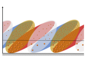
Figure 3. Two-dimensional correlation contours of turbulent velocity fluctuations (a) and dust concentration fluctuations (b) at reference point  $z/\delta = 0.033$ with those at other wall-normal locations, where the blue and red areas are fluctuating streamwise velocity and dust concentration, respectively. The blue and red lines represent the streamwise inclination angles of the fluctuating streamwise velocity and dust concentration, respectively. Contour levels are from 0.05 to 1 in increments of 0.05. The results are from dataset no. 17.
In addition to the instantaneous velocity/concentration fluctuation and the two-point correlation contour, to detect the large-scale structure of dust concentration in particle-laden two-phase flow, the energy spectra demonstrate the distribution of energy at different scales, which can further reflect the importance of the large-scale concentration structure in terms of the energy contribution. Thus, the premultiplied spectra of the velocity fluctuations ( $k_{x}\varPhi _{uu}/U_{\tau }^{2}$) and dust concentration fluctuations ( $k_{x}\varPhi _{cc}/\sigma _{c}^{2}$) in particle-laden flow versus height are given in figures 4(a) and 4(b), respectively (where $k_{x} = 2{\rm \pi} /\lambda _{x}$ is the streamwise wavenumber; $\lambda _{x}$ is the streamwise wavelength; and $\varPhi _{uu}$ and $\varPhi _{cc}$ are the power spectral densities of the streamwise velocity fluctuations and PM10 concentration fluctuations, respectively). The analysis of the premultiplied spectra follows the methods of Kim & Adrian (Reference Kim and Adrian1999), Kunkel & Marusic (Reference Kunkel and Marusic2006) and Vallikivi, Ganapathisubramani & Smits (Reference Vallikivi, Ganapathisubramani and Smits2015). In the premultiplied representation the total area under the curve when integrated against ln( $k_{x}$) (or ln( $\lambda _{x}$)) is equal to the turbulent velocity variance or PM10 concentration variance. The abscissa and ordinate in figure 4(a,b) are normalized by the outer scale $\delta$. It should be noted that there is a difference in the sample frequency between the turbulent velocity and dust concentration. To be consistent with the wavelength range of the $c$ spectra, the proper spatial wavelength range of the $u$ spectra is shown. It can be seen in figure 4(a) that the $u$ spectra are ridge like across the observation ranges. The variation of this ridge (white filled circles) essentially follows $\lambda _{x} \propto (z\delta )^{1/2}$ in the $\lambda _{x}$– $z$ plane. This is consistent with the variation in the wavelength peak of VLSMs with height found by Vallikivi et al. (Reference Vallikivi, Ganapathisubramani and Smits2015), which suggests that the scale of most energy-containing structures in the velocity fluctuation exhibits a simultaneous dependence on local height $z$ and ASL thickness $\delta$. This is because the premultiplied energy spectrum peak corresponds to the $k_{x}^{-1}$ spectra region in the power spectrum, which is derived from the overlap of the low wavenumber regions that usually scale with the outer scale $\delta$ and the intermediate wavenumber range scales well with the local wall-normal distance $z$ in the turbulence spectrum (Perry, Henbest & Chong Reference Perry, Henbest and Chong1986). The dust concentration fluctuation premultiplied spectra shown in figure 4(b) are similar to the spectra of $u$, and there is also a distinct energy ridge (white filled squares). However, the difference is that the energy ridge line varies slightly across all $z$ locations residing in the logarithmic region, approximated by $\lambda _{x} \sim (3-6)\delta$, which is similar to the phenomenon in the pipe flow of $Re_{\tau } \approx 6000$ noted by Pirozzoli et al. (Reference Pirozzoli, Romero, Fatica, Verzicco and Orlandi2022) in which a large-scale temperature fluctuation spectra peak appears and remains invariant with height in the range $z^+=15$ to $z/R = 0.3$. This indicates that the large-scale dust structure is the significant energy-containing and dominant structural feature in the dust concentration field, and the length scale is essentially constant at different measurement heights, which is on the scale of the boundary layer thickness $\delta$ and larger in the logarithmic region. A detailed comparison of the peak wavelengths in the premultiplied spectra of the turbulent velocity fluctuation and dust concentration fluctuation is given in figure 5(b).

Figure 4. Colour contour maps showing variation in one-dimensional premultiplied spectra with the wall-normal position: (a) streamwise velocity fluctuations and (b) dust concentration fluctuations. The results are obtained from dataset no. 17. The white filled circle and square symbols are the corresponding streamwise velocity and dust concentration premultiplied spectra peak, respectively.

Figure 5. Linear coherence cospectra between streamwise velocity fluctuation and dust concentration (a). The variation in peak wavelength versus wall-normal location (b). The results are obtained from dataset nos. 17–21.
Given that large-scale coherent structures exist not only in the flow field but also in the dust concentration field in particle-laden two-phase flow, it is logical to consider how these multiscale two-phase structures relate and affect one another, which can be investigated by means of the linear coherence cospectra between the velocity fluctuations and the dust concentration fluctuations.
Linear coherence spectra are well-established mathematical tools for extracting coherence between structures at different scales in flow fields (Baars, Hutchins & Marusic Reference Baars, Hutchins and Marusic2016; Marusic, Baars & Hutchins Reference Marusic, Baars and Hutchins2017; Baidya et al. Reference Baidya2019; Baars & Marusic Reference Baars and Marusic2020a,Reference Baars and Marusicb) and have been widely used for assessing the self-similarity characteristics of turbulent motions. The basic form is (Baars et al. Reference Baars, Hutchins and Marusic2016, Reference Baars, Hutchins and Marusic2017)
 \begin{equation} \gamma^{2}(z,z_{R};\lambda_{x})=\frac{|\langle\hat{x}(z;\lambda_{x})\hat{x}^{*}(z_{R};\lambda_{x})\rangle|^{2}}{\langle|\hat{x}(z;\lambda_{x})|^{2}\rangle\langle|\hat{x}(z_{R};\lambda_{x})|^{2}\rangle}= \frac{|\varPhi_{xx}^{*}(z,z_{R};\lambda_{x})|^{2}}{\varPhi_{xx}(z;\lambda_{x})\varPhi_{xx}(z_R;\lambda_{x})}, \end{equation}
where  $z$ and $z_{R}$ are the spatial height of any measurement point and the height of the reference point, respectively, and $\hat {x}$ is the Fourier transform of $x$. The asterisk $*$ indicates the complex conjugate, $| {\cdot }|$ designates the modulus and $\langle {\cdot }\rangle$ denotes ensemble averaging. Here $\varPhi _{xx}^{*}(z,z_{R};\lambda _{x})$ and $\varPhi _{xx}^{*}(z;\lambda _{x})$ are the cross-spectra from two different positions ( $z$ and $z_{R}$) and the power spectra at $z$, respectively. Particularly, in this study, the main focus is the scale coherence between the velocity fluctuation and dust concentration signals at the same wall-normal location, i.e. $z_{R} = z$. In this scenario, the formulation of linear coherence cospectra employed here can be expressed as
 \begin{equation} \gamma_{uc}^{2}(z;\lambda_{x})=\frac{|\langle\hat{u}(z;\lambda_{x})\hat{c}^{*}(z;\lambda_{x})\rangle|^{2}}{\langle|\hat{u}(z;\lambda_{x})|^{2}\rangle\langle|\hat{c}(z;\lambda_{x})|^{2}\rangle}= \frac{|\varPhi_{uc}(z;\lambda_{x})|^{2}}{\varPhi_{uu}(z;\lambda_{x})\varPhi_{cc}(z;\lambda_{x})}, \end{equation}
where  $\hat {u}$ and $\hat {c}$ are the Fourier transforms of streamwise velocity fluctuations $u$ and dust concentration fluctuations $c$, respectively. Here $\varPhi _{uu}$, $\varPhi _{cc}$ and $\varPhi _{uc}$ are the energy spectra and cross-spectra of the time series $u$ and $c$, respectively. The linear coherence cospectra is an explicit expression for the ratio of the squared cross-spectra of the two sequences relative to the product of their respective energy spectra (Baars et al. Reference Baars, Hutchins and Marusic2016). The denominator in (3.4) is such that $\gamma ^{2}$ normalization occurs per scale (and, hence, provides the square of the scale-specific correlation coefficient), and for all scales, it is bounded within $0\leq \gamma ^{2}\leq 1$ (Baidya et al. Reference Baidya2019). Here $\gamma ^{2} = 0$ indicates the absence of coherence, while $\gamma ^{2} = 1$ indicates perfect coherence. In terms of the physical meaning, $\gamma ^{2}$ can be interpreted as the square of the scale-specific correlation coefficient, which is equivalent to the two-point correlation in the physical domain and essentially responds to the correlation coefficient at each Fourier component (Baars et al. Reference Baars, Hutchins and Marusic2016, Reference Baars, Hutchins and Marusic2017).
The linear coherence cospectra of the streamwise wind velocity fluctuation and the dust concentration fluctuation at different heights are shown in figure 5(a), where the blue diamond points are the peak values of the spectra. The linear coherence cospectra show the pattern of increasing first and then decreasing with increasing scale at all different heights. The tendency of coherence increasing with scale  $\lambda _{x}$ is consistent with the variation of the LCS of streamwise velocity fluctuation at different heights given by existing studies (Baars et al. Reference Baars, Hutchins and Marusic2016; Baidya et al. Reference Baidya2019; Samie et al. Reference Samie, Baars, Rouhi, Schlatter, Örlü, Marusic and Hutchins2020). This tendency is as anticipated for any spatial two-point measurement with a certain wall-normal separation distance; only vortices with a scale larger than the separation distance are likely to be captured by both measurement points synchronously, so that the signals captured by the two points show coherence, while smaller eddies whose scale are smaller than the separation distance cannot be captured. In other words, as the eddy scale increases, the coherent structures become more easily detected and, therefore, show higher correlation in the spectra (Baars et al. Reference Baars, Hutchins and Marusic2016). Then, the correlation between streamwise velocity fluctuation and dust concentration fluctuation begins to gradually weaken as the wavelength continues to increase. This phenomenon is quite different from the LCS of streamwise velocity fluctuation that appear to level off in the large wavelength range given by Baars et al. (Reference Baars, Hutchins and Marusic2016), Baidya et al. (Reference Baidya2019) and Samie et al. (Reference Samie, Baars, Rouhi, Schlatter, Örlü, Marusic and Hutchins2020). Although Krug et al. (Reference Krug, Baars, Hutchins and Marusic2019) analysed the ASL data from SLTEST, they also found a decay of the spectral line in the LCS of the streamwise velocity fluctuation in the ASL at a large wavelength range, and they concluded that the eventual decay of coherence is likely an artefact of the detrending procedure since a similar effect was not observed in laboratory data. Specifically, some large-scale turbulent fluctuations are inevitably removed in the process of removing long-term trends so that the spectral lines decay at a large wavelength range. However, the decreasing trend of the LCS at very large wavelengths may be plausible. Unlike the LCS of two points at different heights (3.3) given by existing studies (same physical quantity at different heights), the present study provides the LCS between two different physical quantities at the same height (3.4). So, it is not the scale of the eddy that determines the magnitude of the correlation but the effect of turbulent motions on the spatial distribution of dust concentration at different scales. The linear coherence cospectra do not exhibit a gradually slowing increase with the wavelength but first increase and then decrease with a peak, implying that larger turbulent motions do not have a more significant effect on the spatial distribution of the dust concentration; rather, there is turbulent motion that has the most significant effect on the dust spatial distribution, and its size corresponds to the peak scale in the linear coherence cospectra.
Moreover, the colour shift in the curves from blue to red in figure 5(a) corresponds to the increase with the height, and it can be noted that there is a significant difference in the coherence between the velocity fluctuation and the dust concentration fluctuation as the height increases. Here, turbulent motions in the flow field can be divided into three types according to traditional criteria (Guala, Hommema & Adrian Reference Guala, Hommema and Adrian2006; Balakumar & Adrian Reference Balakumar and Adrian2007), namely, SSMs with streamwise scales  $L_{x} < 0.3\delta$, LSMs ( $0.3\delta < L_{x} < 3\delta$) and VLSMs ( $L_{x} > 3\delta$). As seen in figure 5(a), the spectral values of the linear coherence cospectra at different heights remain in the low range (no more than 0.1) in the range of SSMs, indicating that small-scale turbulent motions have less influence on particle concentration fluctuation structures. That is, particles do not follow the small-scale turbulent motions well due to their inertia. In the range of LSMs, the spectral lines increase progressively with the height, reaching a maximum near the middle of the logarithmic region and then decreasing with height as height continues to increase. The spectral lines increase monotonically with increasing height in the range of VLSMs. It can be noted that the tendency of variation presented here is similar to the variation of energy with height, i.e. the energy of VLSMs in the streamwise velocity fluctuations monotonically increases with height in the ASL, while the energy of LSMs slightly increases with height below $z = 0.0233\delta$ and then decreases with height (Wang et al. Reference Wang, Gu and Zheng2020). This may imply that the interphase coherence between velocity fluctuations and dust concentration fluctuations is related to the energy, and turbulent motions with higher energy have higher coherence with the particle concentration.
Figure 5(a) indicates that larger turbulent motions do not have a more significant effect on the spatial distribution of the dust concentration; rather, there is turbulent motion that has the most significant effect on the dust spatial distribution, and its size corresponds to the peak scale in the linear coherence cospectra. There are also clear peaks in the streamwise velocity fluctuation premultiplied energy spectra, which represent the most significant energy-containing turbulent motions. To analyse the relation between the two, the peak scales of the premultiplied energy spectra of the streamwise velocity fluctuation and the dust concentration fluctuation (red and yellow square dots, respectively) are summarized in figure 5(b), with the peak scales of the linear coherence cospectra between the two phases (blue diamonds). Moreover, the results of wavelengths of the energy spectra peak in the laboratory TBL from Balakumar & Adrian (Reference Balakumar and Adrian2007) ( $Re_{\tau }$ = 1476, 2395) and Vallikivi et al. (Reference Vallikivi, Ganapathisubramani and Smits2015) ( $Re_{\tau } = 72\,500$) are also included for comparison. It can be seen in figure 5(b) that the wavelengths of the linear coherence cospectra peak are not only in good agreement with the peak wavelength of the streamwise velocity fluctuation premultiplied energy spectra in this study, but are also in good agreement with the laboratory TBL results at low and medium Reynolds numbers and that both satisfy the 1/2 power scaling law of the product of local height $z$ and ASL thickness $\delta$, indicating that the structures of the flow field with the most significant energy dominate the spatial distribution of the dust concentration. However, the wavelengths associated with the dust concentration fluctuation premultiplied spectra peak are larger than those of the streamwise velocity fluctuation at lower heights. This difference decreases with increasing height, and the wavelengths are essentially the same near the top of the logarithmic region. This phenomenon is consistent with that observed in the two-point correlation contour (see figure 3), where the length scale of the near-wall dust concentration structures is larger than that of the turbulent motions.
4. Interphase amplitude modulation
The existence of dust concentration structures in particle-laden flow has been confirmed, and the strength of the linear coherence between the two phases at different scales is analysed by using linear coherence cospectra in § 3. In this section the nonlinear modulation effect of streamwise velocity fluctuation on the sand and dust concentration fluctuation is further analysed by means of the amplitude modulation coefficient. To visualize the modulation effect of the streamwise velocity fluctuation on the dust concentration fluctuation, the time series of the small-scale fluctuation  $c_{S}(t)$ ( $\lambda _{x} < \delta$) of the dust concentration in the outer region ( $z/\delta \approx 0.2$) and the small-scale fluctuation $q_{S}(t)$ ( $\lambda _{x} < \delta$) of the saltating particle mass flux in the near-wall region ( $z/\delta \approx 0.0002$) are presented in figures 6(a) and 6(b), respectively, along with the corresponding large-scale streamwise velocity fluctuations $u_{L}(t)$ ( $\lambda _{x}> \delta$) obtained synchronously at the same height. The velocity fluctuation is normalized by the inner-scaling friction velocity $U_{\tau }$, denoted by the superscript ‘+’. The dust concentration and sand flux are normalized by the corresponding root mean square of the fluctuations (Wang et al. Reference Wang, Zheng and Tao2017; Talluru et al. Reference Talluru, Philip and Chauhan2018; Chowdhuri & Prabha Reference Chowdhuri and Prabha2019). Figure 6(a) shows the time series of the concentrations of suspended small dust particles at higher locations with the same streamwise velocity fluctuations measured synchronously. The amplitude of the concentration fluctuation for suspended dust with small particle size at higher locations is strongly dependent on the large-scale streamwise velocity fluctuations. When the large-scale velocity fluctuations are positive ( $u_{L} > 0$, within the red region), the small scales of dust are increasingly quiescent, whereas when the large-scale fluctuation is negative ( $u_{L} < 0$, within the blue region), the amplitude of the small-scale dust concentration fluctuations measured synchronously is larger. For the larger particles near the wall, see figure 6(b), the results are the opposite: when the large-scale velocity fluctuation is positive ( $u_{L} > 0$, red region), the intensity of the mass flux fluctuation $q_{S}$ of the small-scale saltating particles increases, and when the large-scale velocity fluctuation is negative ( $u_{L} < 0$, blue region), the intensity of the small-scale saltating particle flux fluctuation decreases. The results are similar to the phenomenon described in Hutchins & Marusic (Reference Hutchins and Marusic2007) and Mathis et al. (Reference Mathis, Hutchins and Marusic2009a) for the amplitude modulation of the large-scale component of streamwise velocity fluctuation on small scales. In the near-wall region the amplitude of small scales is more active in positive large-scale velocity fluctuations, while with increasing height, the amplitude of small scales is more active in negative large-scale components. Therefore, the strength of the sand and dust concentration fluctuation is closely related to the large-scale turbulent fluctuations, and the fluid phase exerts a significant amplitude (energy) modulation on the particle concentration fluctuations. It seems significantly energetic saltating sand particles near the wall preferentially accumulate in the high-speed region of the flow field, while at higher positions, suspended dust particles are present in the low-speed region of the flow field.

Figure 6. Example of fluctuating turbulent velocity signals and particle concentration signals. (a) Outer large-scale ( $\lambda _{x} > \delta$) streamwise velocity fluctuation $u_{L}$ and small-scale ( $\lambda _{x} < \delta$) dust concentration fluctuation $c_{S}$ at $z/\delta = 0.2$ from dataset no. 17. (b) Inner large-scale streamwise velocity fluctuation and small-scale ( $\lambda _{x} < \delta$) particle (particle size is within 30–480 $\mathrm {\mu }$m) mass flux fluctuation $q_{S}$ near wall $z/\delta = 2 \times 10^{-4}$ from dataset no. 25. The symbol $+$ indicates inner scaling; $u^+ = u/U_{\tau }$; $t^+=tU_{\tau }^{2}/\nu$; and $\sigma _{c}$ and $\sigma _{q}$ are the root mean square of dust concentration fluctuation and particle mass flux, respectively.
Figure 6 shows that the amplitude of the concentration fluctuations in larger saltating particles and in smaller suspended dust is closely related to the large-scale turbulent motion, implying that the large-scale turbulent motions directly influence the spatial distribution characteristics of the particle concentration in the particle-laden two-phase flow. To quantify the degree of the amplitude modulation of the fluid onto particle concentration, the amplitude modulation coefficient (referred to as the interphase amplitude modulation coefficient) of large-scale velocity fluctuations on small-scale particle concentration fluctuations and its variation are considered by referring to and extending the definition of the single-point amplitude modulation coefficient developed by Mathis et al. (Reference Mathis, Hutchins and Marusic2009a). The calculation procedure for the interphase amplitude modulation coefficient is outlined below. First, the streamwise velocity fluctuation  $u(t; z)$ and the dust concentration fluctuation $c(t; z)$ or mass flux fluctuation $q(t; z)$ at the same height are converted from the time domain to the frequency domain by Fourier transform, combined with the Taylor's frozen hypothesis, and the corresponding wavelengths are obtained based on the frequencies,
 \begin{gather} \hat{u}(\lambda_{x};z) = \mathscr{F}[u(t; z)], \end{gather}
 \begin{gather} \hat{c}(\lambda_{x};z) = \mathscr{F}[c(t; z)], \end{gather}
 \begin{gather} \hat{q}(\lambda_{x};z) = \mathscr{F}[q(t; z)]. \end{gather}
On this basis, the cutoff wavelength  $\lambda _{c}$ is required to obtain large-scale fluctuating streamwise velocity signals as well as small-scale fluctuating particle concentration/mass flux signals. In the existing studies on amplitude modulation, a single filter wavelength is commonly used to classify the large-scale and small-scale components (Mathis et al. Reference Mathis, Hutchins and Marusic2009a; Schlatter & Örlü Reference Schlatter and Örlü2010; Bernardini & Pirozzoli Reference Bernardini and Pirozzoli2011; Talluru et al. Reference Talluru, Baidya, Hutchins and Marusic2014; Baars et al. Reference Baars, Talluru, Hutchins and Marusic2015; Pathikonda & Christensen Reference Pathikonda and Christensen2017). The decomposition used in Mathis et al. (Reference Mathis, Hutchins and Marusic2009a) is based on a cutoff wavelength that is selected from the premultiplied energy spectra map. The cutoff $\lambda _{x}/\delta = 1$ appears to be a location that clearly separates the two distinct peaks of the large- and small-scale components of the fluctuating $u$ signal. In addition, Liu et al. (Reference Liu, Wang and Zheng2019) further systematically analysed the multiscale effect on amplitude modulation. The most energetic motions with scales larger than the wavelength of the lower wavenumber peak in the energy spectra play a vital role in the amplitude modulation effect, whereas the motions with scales shorter than the wavelength of the higher wavenumber peak are strongly modulated. In this study the structure scales at which the fluid phase has the most significant influence on the particle phase are investigated in § 3 through the peak in the linear coherence cospectra. These wavelengths correspond to the peak wavelength of the premultiplied energy spectrum of the streamwise velocity fluctuations. Thus, this wavelength is employed here as the cutoff wavelength for the decoupling process, i.e.
 \begin{equation} \lambda_{c}(z) = \lambda_{x}(z)|_{(\max\gamma_{uc(uq)}^{2})}. \end{equation}
Furthermore, the large-scale component of the fluctuating streamwise velocity and the small-scale component of the fluctuating particle concentration can be obtained via inverse Fourier transform, i.e.
 \begin{gather} u_{L}(t;z)=\mathscr{F}^{-1}\left[\left.\hat{u}(\lambda_{x};z)\right|_{\lambda_{x}>\lambda_{c}}\right], \end{gather}
 \begin{gather} c_{S}(t;z)=\mathscr{F}^{-1}\left[\left.\hat{c}\left(\lambda_{x};z\right)\right|_{\lambda_{x}<\lambda_{c}}\right], \end{gather}
 \begin{gather} q_{S}(t;z)=\mathscr{F}^{-1}\left[\left.\hat{q}(\lambda_{x};z)\right|_{\lambda_{x}<\lambda_{c}}\right]. \end{gather}
Then, the envelope  $E(c_{S}(t;z))$ and $E(q_{S}(t;z))$ returned by the Hilbert transformation tracks the amplitude variation of the small-scale components, and the amplitude modulation due to the large-scale turbulent motions can be presented as
 \begin{gather} E_{L}(c_{S}(t;z))=\mathscr{F}^{-1}\left\{\left.\mathscr{F}\left[E(c_{S}(t;z))\right]\right|_{\lambda_{x}>\lambda_{c}}\right\}, \end{gather}
 \begin{gather} E_{L}(q_{S}(t;z))=\mathscr{F}^{-1}\left\{\left.\mathscr{F}\left[E(q_{S}(t;z))\right]\right|_{\lambda_{x}>\lambda_{c}}\right\}. \end{gather}
Finally, the amplitude modulation effect of large-scale streamwise velocity fluctuations on small-scale particle concentration fluctuations obtained at the same height (i.e. one-point amplitude modulation) can be quantified by calculating the correlation coefficient between the two, i.e.
 \begin{equation} R_{AM}(z)=\frac{\overline{u_{L}(z) E_{L}(c_{S}(z))}}{\sqrt{\overline{{u_{L}(z)}^{2}}} \sqrt{\overline{E_{L}(c_{S}(z))^{2}}}}, \end{equation}
and
 \begin{equation} R_{AM}(z)=\frac{\overline{u_{L}(z) E_{L}(q_{S}(z))}}{\sqrt{\overline{{u_{L}(z)}^{2}}} \sqrt{\overline{E_{L}(q_{S}(z))^{2}}}}. \end{equation}
To investigate whether the amplitude modulation effect of the turbulent velocity fluctuation on the particle concentration fluctuation is related to the concentration scale, the amplitude modulation coefficient as a function of the particle concentration cutoff wavelength is first calculated. The results are presented in figure 7(a) at the positions  $z/\delta = 0.006$ and $z/\delta = 0.2$, respectively. Within the experimental error, the $R_{AM}$ values in figure 7(a) are found to be invariant with the outer-scaled cutoff wavelength $\lambda _{c}/\delta$. This phenomenon is quite different from the amplitude modulation of turbulent motions with different cutoff wavelengths on SSMs, for which $R_{AM}$ exhibits a gradually slowing increase as the cutoff wavelength decreases and then appears to level off. The amplitude modulation of the turbulent motions onto particle concentration shows no significant variance with the cutoff wavelength, implying that $R_{AM}$ has no dependence on the scale of the particle concentration. In view of this, the full-scale information, not the small-scale component of the particle concentration, is used in the subsequent investigation.

Figure 7. Amplitude modulation coefficient of large-scale streamwise velocity fluctuation on dust concentration fluctuation at different scales (a). Variation in the interphase amplitude modulation coefficient with height (b). The red and blue regions are the saltation layer and the suspension layer, respectively. The blue filled square dots and red filled symbols are the amplitude modulation coefficients of fluctuating streamwise velocity to particle concentration fluctuations, and the yellow filled symbols represent the amplitude modulation of large-scale turbulent velocity components to small scales. The results are averaged from dataset nos. 15–21, and the corresponding error bars represent the standard error. The white filled symbols are the turbulent velocity amplitude modulation in particle-free flows in Liu et al. (Reference Liu, Wang and Zheng2019).
To give one-point interphase amplitude modulation coefficients at different heights over the entire measurement range, the decoupling procedure is applied to all of the wall-normal measurement stations across the saltation and suspension layers. The interphase amplitude modulation coefficients of the large-scale streamwise velocity fluctuations on the particle (dust as well as saltating particles) concentration fluctuations are obtained, and their variations with wall-normal location can be observed in figure 7(b), where the red area indicates the particle saltation layer and the blue area is the suspension layer. For comparison with the flow field results, the amplitude modulation coefficients for the large-scale streamwise velocity fluctuations to small scales in the ASL data in this study are also shown in figure 7(b).
As seen from the red filled symbols in figure 7(b), the amplitude modulation coefficient between the streamwise velocity fluctuation and the sand transport flux fluctuation of the saltating particles can be achieved up to 0.25 at near-wall locations, and the amplitude modulation coefficient decreases progressively to reach a zero value near the top of the saltation layer. At higher locations, the degree of the amplitude modulation of the large-scale turbulent velocity fluctuations on the small-size dust concentration fluctuations follows the overall trend of decreasing with height, and a reversal in the amplitude modulation behaviour can be observed in figure 7(b), i.e. the amplitude modulation coefficient shows negative values. It reveals that the amplitude of the small-size dust concentration is significantly reduced within large-scale positive fluctuations and the opposite scenario can be found within the large-scale negative fluctuations. In addition, the amplitude modulation of large-scale turbulent motions on particles with different sizes shows obvious differences at the same location. The comparison of the two types of particles is shown in the black square in figure 7(b), and the amplitude modulation on small dust (PM10 with  $St_{\eta } \sim O(10^{-2})$) collected by DUSTTRACK is stronger than that on larger particles (sizes spanning $30\unicode{x2013}480\,\mathrm {\mu }{\rm m}$, $St_{\eta } \sim O(10^{-1})\unicode{x2013}O(10^{1})$) collected by SPC. It is understandable when taking the $St$ number of particles into consideration that small-scale dust with a smaller $St$ number (smaller particle relaxation time) can follow smaller-scale turbulent motions than larger particles; i.e. small dust particles retain the nature of small-scale turbulent motions to some extent, whereas large particles can follow only LSMs. The absence of SSMs that are subject to the amplitude modulation effect (carrier signals) leads to a decrease in the amplitude modulation coefficient (Liu et al. Reference Liu, Wang and Zheng2019). It also indicates that dust associated with smaller-scale turbulent motions is modulated by large-scale turbulent motions more significantly than large particles associated with larger-scale turbulent motions.
When compared with the amplitude modulation coefficients of the large-scale streamwise velocity fluctuations to small-scale components  $R_{AM}^{uu}$, the amplitude modulation coefficient to particle concentration fluctuations $R_{AM}^{uc}$ is significantly smaller than $R_{AM}^{uu}$, which can be explained by the particle inertia. Although small dust particles have a smaller $St$ number and less particle inertia, particles ( $St^+ \gg 1$) still cannot perfectly follow the very small-scale turbulent fluctuations that are significantly modulated by VLSMs, so the interphase amplitude modulation coefficient is reduced by omitting some of the small-scale carrier signals. The reduced degree of the amplitude modulation makes a significant difference on the locations where the interphase amplitude modulation coefficient $R_{AM}^{uc}$ is approximately zero compared with those of the amplitude modulation coefficients for multiscale turbulent motions $R_{AM}^{uu}$. The location of the reversal behaviour observed in interphase amplitude modulation is approximately at the top of the saltation layer, while the reversal of the traditional amplitude modulation within turbulent motions corresponds reasonably well with the location of the outer peak of the energy spectra that agrees well with the nominal midpoint of the log region (Mathis et al. Reference Mathis, Hutchins and Marusic2009a). In addition, the modulation effect of the large-scale streamwise velocity fluctuation on small scales in the particle-laden flow in this study is much smaller than the results given by existing studies in particle-free flow at high Reynolds numbers (Liu et al. Reference Liu, Wang and Zheng2019), which is consistent with the tendency of the amplitude modulation coefficient reduction in particle-laden flows indicated by Liu et al. (Reference Liu, He and Zheng2023).
Given that the natural interpretation of a correlation coefficient is that of an inner product (see Rodgers & Nicewander Reference Rodgers and Nicewander1988, for details), the amplitude modulation coefficient  $R_{AM}$ actually represents the phase angle, $\Delta \varphi$, between the two signals, i.e. $R_{AM} = \cos (\Delta \varphi )$ (Chung & McKeon Reference Chung and McKeon2010; Jacobi & McKeon Reference Jacobi and McKeon2013; Jacobi et al. Reference Jacobi, Chung, Duvvuri and McKeon2021). The amplitude modulation coefficient, compared with the traditional correlation coefficient, not only quantifies the relationship between the nonlinear modulation imprint on the particle concentrations and the large-scale turbulent motions but also characterizes the spatial relationship between the particle concentration and turbulent motions. Therefore, this equation allows the amplitude modulation coefficient shown in figure 7(b) to be converted into the phase difference, and the phase relationship between the fluid phase and the particle phase over the entire observation range can be investigated. The obtained results are shown in figure 8(a). The phase difference (yellow filled points) increases monotonically and in a linear-log manner with the wall-normal location over the entire observation range. The phase difference between the large-scale turbulent velocity fluctuations and the mass flux fluctuations of the saltating particles is less than ${\rm \pi} /2$ throughout the saltation layer. The phase difference becomes larger as the wall-normal location increases, and it gradually reaches approximately ${\rm \pi} /2$ near the top of the saltation layer. In the suspension layer above the saltation layer, the difference between the two is greater than ${\rm \pi} /2$, and it continues to increase progressively with increasing height.

Figure 8. (a) The variation in phase difference  $\Delta \varphi$ between large-scale turbulent velocity fluctuations and particle concentration fluctuations with the wall-normal location ( $z/\delta$, $z^+$), where the red and blue regions are the saltation layer and the suspension layer, respectively. The yellow filled circles and square symbols are the phase difference for dust and saltating particles, respectively. The results are averaged from dataset nos. 15 to 21 and nos. 22 to 26, and the corresponding error bars represent the standard error. (b) Map of the temporal cross-correlation function $R_{AM}(z; \Delta t)$ with the peaks marked.
However, it should be noted that although the phase difference relationship between the large-scale turbulent velocity fluctuation and particle concentration fluctuation is currently established, the sign of the phase,  $\Delta \varphi$, is lost due to the symmetry of the cosine function. Consequently, the precise nature of the phase relationship remains ambiguous. This method is not capable of indicating the backwards or forwards spatial relationship between the two (Jacobi & McKeon Reference Jacobi and McKeon2013). To obtain the correct sign of the phase difference and thus further infer the actual physical orientation of the two, the amplitude modulation function with temporal information $\Delta t$ must be employed, i.e.
 \begin{equation} R_{AM}(z; \Delta t)=\frac{\overline{u_{L}(z; \Delta t) E_{L}(c(z))}}{\sqrt{\overline{{u_{L}(z; \Delta t)}^{2}}} \sqrt{\overline{E_{L}(c(z))^{2}}}}. \end{equation}
The relative phase lag between the two signals can be inferred by tracking the variation in the peak position of the amplitude modulation coefficient. The results are shown in figure 8(b), where the black dashed line is the amplitude modulation coefficient of the large-scale streamwise velocity fluctuation on the dust concentration fluctuation as well as the sand mass flux fluctuation near the wall shown in figure 7 above. Based on the results presented in figure 8(a,b), the phase lag over the whole range of observations (the saltation layer and suspension layer) is found to be negative, indicating that the large-scale velocity fluctuations lead to particle fluctuations in a temporal (i.e. physical) sense. In detail, in the near-wall saltation layer the phase difference between the large-scale streamwise velocity fluctuation and the sand mass flux fluctuation is quite small. With increasing height, the streamwise velocity fluctuation gradually leads to particle concentration fluctuation. In other words, the phase difference between the two gradually increases, and the modulation coefficient approaches 0 at the top of the saltation layer (the phase difference between the two structures is close to  ${\rm \pi} /2$). As the height continues to increase, this leading degree becomes increasingly significant. This tendency indicates that the turbulent velocity motions always tend to lead the particle cluster structures throughout the whole observation range, and this leading effect becomes increasingly obvious with increasing height.
5. Relationship between the spatial distribution of dust concentration and turbulent motions
It can be seen that the large-scale streamwise velocity fluctuation has a significant amplitude modulation effect on the fluctuation in the transport intensity of the saltating sand particles and fluctuation in the dust concentration throughout the whole observation region (saltation layer and suspension layer), as shown in figure 9(a). Based on the above-discussed modulation coefficients and phase differences between the large-scale streamwise velocity and particle concentration structures, the relative phase of the two types of structures can be conveniently and effectively refined. The results are shown in figure 9(b). The red and blue colours are the high-speed region and low-speed region, respectively. The yellow filled region is the particle clustering structure, the white region is the low-concentration region appearing at intervals, and  $z_{c}$ is the saltation layer height. Near the wall, the phase difference between the saltation particle structure and the turbulent velocity motions is quite small and gradually increases with increasing height. The phase difference reaches ${\rm \pi} /2$ at the top of the saltation layer. In the suspension layer above the saltation layer, the dust concentration forms an obvious coherent structure. The phase difference between the dust concentration and the turbulent streamwise velocity starts at ${\rm \pi} /2$ and exceeds ${\rm \pi} /2$ by increasing approximately logarithmically with the height, which means that the relative inclination of the large-scale turbulent motions is steeper than that of the particle concentration.

Figure 9. (a) Schematic diagram of the effect of amplitude modulation ( $R_{AM} < 0$); (b) schematic representation of the relative orientations of turbulent velocity and particle concentration.
Furthermore, synchronous data on streamwise velocity fluctuations and dust concentration (particle mass flux) fluctuations are used to calculate the joint probability density function (j.p.d.f.) of the two in quadrant space (Wallace Reference Wallace2016) to validate the correctness of the particle–turbulence phase relationship model proposed above. Mathematically, the j.p.d.f. can be expressed as
 \begin{equation} P_{u^{{\ast}}c^{{\ast}}} = \frac{N_i}{N\,{\rm d}u^{{\ast}}\,{\rm d}c^{{\ast}}}, \end{equation}
where ‘ $\ast$’ represents the normalization with the standard deviation $\sigma$, $P_{u^{\ast }c^{\ast }}$ is the j.p.d.f. of the two variables $(u^{\ast },c^{\ast })$, $N$ is the total number of points in a single run, $N_{i}$ is the number of points in the $i$th pixel of ${\rm d}u^{\ast }\,{\rm d}c^{\ast }$, and ${\rm d}u^{\ast }$ and ${\rm d}c^{\ast }$ are the length and width of the pixel, respectively. The length and width are defined by the equations
 \begin{gather} {\rm d}u^{{\ast}} = \frac{u_{max}^{{\ast}}-u_{min}^{{\ast}}}{bin_{u^{{\ast}}}}, \end{gather}
 \begin{gather} {\rm d}c^{{\ast}} = \frac{c_{max}^{{\ast}}-c_{min}^{{\ast}}}{bin_{c^{{\ast}}}}, \end{gather}
where  $u_{max}^{\ast }$ and $u_{min}^{\ast }$ are the maximum and minimum values of the $u^{\ast }$ time series, and similarly, $c_{max}^{\ast }$ and $c_{min}^{\ast }$ are the maximum and minimum values of the $c^{\ast }$ time series. Here $bin_{u^{\ast }}$ and $bin_{c^{\ast }}$ are the numbers of bins chosen, which are both 40. The distribution of the time series $u^{\ast }$ and $c^{\ast }$ in the $u^{\ast }$– $c^{\ast }$ plane provides the opportunity to capture the contribution of the quadrant event over the entire time interval visually and efficiently:
 \begin{equation} \iint P_{u^{{\ast}}c^{{\ast}}}\,{\rm d}u^{{\ast}}\,{\rm d}c^{{\ast}}=1. \end{equation}
The j.p.d.f. of the streamwise velocity fluctuation and dust concentration (particle mass flux) at different heights are shown in figure 10(a–d), where figure 10(a,b) shows the results within the near-wall saltation layers  $z^+ \approx 700$ and 6533, and figure 10(c,d) shows the results for the suspension layers $z/\delta \approx 0.006$ and 0.2, respectively. From its general trend, the j.p.d.f. distribution in different quadrants changes significantly with increasing height. The j.p.d.f. distribution exhibits a significant long axis pointing to the first and third quadrants ( ${\rm Q}_{1}$ and ${\rm Q}_{3}$) in figure 10(a) and gradually changes to an approximately circular distribution (shown in figure 10b). Then, in figure 10(c,d) there tends to be a significant distribution with the long axis pointing to the second and fourth quadrants ( ${\rm Q}_{2}$ and ${\rm Q}_{4}$) at the top of the logarithmic region. The variation implies that the preferential accumulation characteristics of sand and dust particles in the high-speed and low-speed regions change significantly with increasing height in the wind-blown sand two-phase flow.

Figure 10. Joint probability density contours for the fluctuating streamwise velocity and dust concentration (mass flux). Plots (a,b) are the j.p.d.f.s obtained from dataset no. 25 at  $z^+ \approx 700$ and 6533 in the saltation layer, respectively. Plots (c,d) are the j.p.d.f.s obtained from dataset no. 17 at $z/\delta$ and 0.2 in the suspension layer, respectively. The corresponding probability in each quadrant is shown to reflect the joint contribution of the entire quadrant.
Specifically, the probability of positive  $q_{f}$ in ${\rm Q}_{1}$ (0.23) is quite a bit larger than that in ${\rm Q}_{2}$ (0.19), in the same way, for negative $q_{f}$, the probability is larger in ${\rm Q}_{3}$ (0.30) than in ${\rm Q}_{4}$ (0.28). It implies that high-concentration saltating particles are more likely to be located in the turbulent high-speed region, while the low-concentration structures are located in the turbulent low-speed region. As indicated by the interphase structure relationship in figure 9, the yellow high-concentration saltating particle structure in the near-wall region nearly overlaps with the red high-speed structure. As the height increases, this relationship becomes less obvious (see figure 10b,c), which is reflected in figure 9 as the high-concentration particle structure shown in yellow gradually deviates from the red high-speed region, indicating that the particle concentration spatial structure does not have a preferential tendency to be distributed in the high-speed or low-speed region. As the height continues to increase, the j.p.d.f. distribution gradually tilts towards the ${\rm Q}_{2}$ and ${\rm Q}_{4}$ quadrants (see figure 10d), the corresponding probability is approximately 0.24 and 0.38, which is quite a bit larger than the probabilities in ${\rm Q}_{1}$ (0.12) and ${\rm Q}_{3}$ (0.26), respectively. It implies that at approximately the top of the logarithmic region, the high-concentration dust particles tend to accumulate in the low-speed region of the fluid, while the lower-concentration dust is in the high-speed region of the fluid. This corresponds to the tendency of the yellow high-concentration dust structure and the blue low-speed streamwise velocity structure to gradually approach each other with increasing height in the suspension layer, as shown by the interphase structure relationship. The results for dust particles are consistent with the descriptions in the studies on the spatial distribution of different particles, which indicate that small particles tend to accumulate in the low-speed region of the fluid (McLaughlin Reference McLaughlin1989; Eaton & Fessler Reference Eaton and Fessler1994; Brandt & Coletti Reference Brandt and Coletti2022). However, the results for saltating particles are quite different from the studies in solid wall, but they are consistent with the results on the erodible surface (Wang et al. Reference Wang, Feng, Zheng and Sung2019), where saltating particles tend to aggregate in the large-scale turbulent high-speed region due to the footprint of the large-scale turbulent motion sweeping down to the flat and erodible surface.
Based on the particle–turbulent phase relationship obtained in figure 9(b), the inclination angle between turbulent structures and particle structures is further explored in conjunction with the fact that a certain inclination degree exists between the large-scale streamwise velocity fluctuation structure and the wall in the existing study. By simplifying the interphase relationship model shown in figure 9, a schematic representation of the inclination angle of the VLSMs  $\gamma _{f}$ and the inclination angle of the dust concentration $\gamma _{p}$ in this process can be obtained and shown in figure 11(a), where $\Delta z$ is the height difference between the highest point of the VLSMs, the height of the reference point is approximated as the near-wall saltation layer where the phase difference is approximately ${\rm \pi} /2$ and $\Delta x$ is the offset of the turbulent structure from the particle concentration structure in the streamwise direction. A simple triangular relationship is expressed as
 \begin{equation} \frac{\Delta z}{\tan \gamma_{f}}=\frac{\Delta z}{\tan \gamma_{p}}+\Delta x. \end{equation}
Figure 11. (a) Simplified representation of the turbulent velocity structure inclination angle and particle cluster inclination angle in the flow field. (b) A packet of  $\varLambda$ hairpin vortices with nine individual $\varLambda$ hairpin vortices, where $\gamma _{f}$ is the inclination of the packet and $U_{c}$ is the convection velocity. (c) Successive hairpin vortices in a large structure with a characteristic upstream interface slope.
To investigate the relationship between  $\Delta z$ and $\Delta x$, the hairpin vortex packet model (Adrian et al. Reference Adrian, Meinhart and Tomkins2000) is used for analysis. The hairpin vortex is the main coherent structure in the flow field, whose characteristic angle is $45^{\circ }$ to the wall (Bandyopadhyay Reference Bandyopadhyay1980; Dennis Reference Dennis2015). The hairpin vortices and the induced secondary hairpins are aligned coherently in the streamwise direction, creating a larger-scale coherent motion called the hairpin vortex packet (Bandyopadhyay Reference Bandyopadhyay1980; Adrian et al. Reference Adrian, Meinhart and Tomkins2000; Christensen & Adrian Reference Christensen and Adrian2001). With the ramp-like pattern in its morphology, the hairpins occur in groups whose heads describe an envelope inclined at $15^{\circ }\unicode{x2013}20^{\circ }$ with respect to the wall, as shown in figure 11(b).
Based on Bandyopadhyay (Reference Bandyopadhyay1980)'s consideration of the dynamics of a hairpin vortex in the streamwise direction, two different hierarchy levels of the hairpin vortex within the large structure are considered in figure 11(c) (here the shape of the vortex is plotted as  $\varLambda$, noting that the shape of the vortex does not affect the results of this study). The smallest upstream and downstream vortices have lengths of $BB'$ and $AA'$, respectively, and $\Delta t$ represents the time interval between the formation of $BB'$ and $AA'$. A sequence of large-scale velocity fluctuations in the flow field is assumed to have a period $T$ (which contains a large-scale high-speed structure and a large-scale low-speed structure). The convective velocity is $U_{c}$, and $L_{x}$ is the streamwise scale of the large-scale structure. The streamwise lengths of the low-speed and high-speed structures in the flow field are approximately the same (Dennis & Nickels Reference Dennis and Nickels2011; Baltzer et al. Reference Baltzer, Adrian and Wu2013), so the streamwise lengths of the low- and high-speed structures are not strictly distinguished and are uniformly called $L_{x}$ for large-scale structures. The relationship between streamwise length $L_{x}$ and period $T$ can be expressed as
 \begin{equation} 2L_{x}=U_{c}T. \end{equation}
From the hairpin vortex packet theory, it is clear that the spacing of the hairpin vortices determines the streamwise scale of the large-scale turbulent structure; then, according to figure 11(c),
 \begin{gather} BD = L_{x} = U_{c}\Delta t, \end{gather}
 \begin{gather} \Delta t = \frac{L_{x}}{U_{c}}=\frac{T}{2}. \end{gather}
Hairpin vortex  $AA'$ has grown by $AD$ during $\Delta t$, so
 \begin{equation} AD = U_{c}\cos45^{{\circ}}\Delta t. \end{equation}
Then, the growth distance in the wall-normal direction can be expressed as
 \begin{equation} \Delta z =AD\sin 45^{{\circ}}. \end{equation}
The phase difference between the large-scale streamwise velocity fluctuation and dust concentration fluctuation structure is approximately  ${\rm \pi} /2$ at the saltation layer, as previously established in the interphase relationship model; therefore,
 \begin{equation} \Delta x = U_{c}\frac{{\rm \pi}/2}{2{\rm \pi}}T=\frac{1}{4}U_{c}T. \end{equation}
With the incorporation of (5.10) and (5.11) into (5.5), after simplification,
 \begin{equation} \frac{1}{\tan \gamma_{f}}=\frac{1}{\tan \gamma_{p}}+1, \end{equation}
which characterizes the inclination angle relationship between the large-scale velocity structure and the particle clustering structure in wind-blown sand two-phase flow.
On the basis of qualitatively giving the spatial structure morphology of turbulence velocity and particle concentration and analysing the spatial relationship between the two structures, the inclination angle relationship between the coherent structures of the two is further verified. There is a large amount of research on the structure inclination angle of turbulent coherent structures (Marusic & Heuer Reference Marusic and Heuer2007; Wu & Christensen Reference Wu and Christensen2010; Chauhan et al. Reference Chauhan, Hutchins, Monty and Marusic2013; Liu et al. Reference Liu, Bo and Liang2017). Here, the whole calculation process is illustrated by the cross-correlation of the particle concentration fluctuation  $c$. Figure 12(a) shows the two-point correlation of the fluctuating dust concentration signal $c$ from the lowest wall-normal position $z_{R}/\delta = 0.006$ with the $c$ signal from the remaining wall-normal array sonic anemometers. With increasing $\Delta z$, the peak correlation magnitude decreases (black dots in figure 12a). In addition, with decreasing peak $R_{cc}$, an obvious shift in the peak location away from the reference point is observed, which represents the spatial delay, i.e. $\Delta x^{*}$. This shift extent becomes larger as $\Delta z$ increases, which is consistent with the cross-correlation in streamwise velocity fluctuation (Guala et al. Reference Guala, Metzger and McKeon2011; Liu et al. Reference Liu, Bo and Liang2017). Referring to the calculation methods in the existing study for the structure inclination angle, the structure inclination angle of the dust concentration can be determined by calculating the spatial delay of the peak location in $R_{cc}$ at two different heights,
 \begin{equation} \gamma_{p}=\arctan(\langle\Delta z/\Delta x^{*}\rangle), \end{equation}
which has been widely used to calculate the structure inclination angle of streamwise velocity fluctuations.

Figure 12. (a) Two-point correlation  $R_{cc}$ of the $c$ signal from the lowest wall-normal position $z_{R}/\delta = 0.006$ with the $c$ signal from the remaining wall-normal array sonic anemometers. Black dots indicate peak $R_{cc}$ at every wall-normal location. (b) The relationship between the turbulent velocity structure inclination angle $\gamma _{f}$ and the particle cluster inclination angle $\gamma _{p}$ obtained from the two-point correlation of $R_{uu}$ and $R_{cc}$. The black line is the derived result from (5.12), and the grey shaded area denotes the standard error $\pm 5^{\circ }$. The results are from dataset nos. 1–21. The yellow filled square symbols are the observational results from Wang et al. (Reference Wang, Gu and Zheng2020).
The large-scale turbulence structure inclination angle  $\gamma _{f}$ and the corresponding dust clustering structure inclination angle $\gamma _{p}$ are plotted as the abscissa and ordinate, respectively, in figure 12(b) based on the synchronous data of turbulent velocity and dust concentration measured at the QLOA (nos. 1–21 in table 2). In this figure, the symbols are experimental results, the black line is the calculated result from (5.12) and the grey shaded area denotes the standard error $\pm 5^{\circ }$ obtained from the calculation of the structure inclination angle in Liu et al. (Reference Liu, Bo and Liang2017). It can be seen in figure 12(b) that within the expected experimental scatter, the calculated result from (5.12) is not only in good agreement with the experimental results obtained from the data in this study but also with the results given in the research on wind-blown sand two-phase flows (Wang et al. Reference Wang, Gu and Zheng2020). This agreement indicates that (5.12) derived from the hairpin vortex model and the particle–turbulence phase relationship can well characterize the inclination angle relationship between the large-scale turbulent velocity structure and particle clustering structure in wind-blown sand two-phase flows. In addition, the large-scale turbulent structure inclination angle varies in the range of $14^{\circ }$– $18^{\circ }$ for near-neutral stratified conditions at low particle mass loading ( $\varPhi _{m} < 1.74 \times 10^{-5}$), which is consistent with the results of particle-free TBL experiments ( $Re_{\tau } \leq O(10^{3})$) (Brown & Thomas Reference Brown and Thomas1977; Christensen & Adrian Reference Christensen and Adrian2001; Marusic & Heuer Reference Marusic and Heuer2007) and ASL observations ( $Re_{\tau } \sim O(10^{6})$) (Morris et al. Reference Morris, Stolpa, Slaboch and Klewicki2007; Guala et al. Reference Guala, Metzger and McKeon2011) that exhibit a range of structure inclination angles under near-neutral stratified conditions ( $11^{\circ }$– $18^{\circ }$). As the particle mass loading increases, the turbulent structure inclination angle increases, which is also consistent with the existing findings from particle-laden experiments (Tay et al. Reference Tay, Kuhn and Tachie2015) and field observations (Wang et al. Reference Wang, Gu and Zheng2020) that indicate particles increase the structure inclination angle.
Table 2. Key information on the datasets in particle-laden ASL. The particle mass loading is estimated at  $z = 0.9$ m (dataset nos. 1–21) and $z = 0.03$ m (dataset nos. 22–26).

6. Conclusion and remarks
Based on the turbulent velocity and particle concentration data obtained synchronously at QLOA, the effect of turbulent motions on particle distribution is investigated. It is found that very-large-scale structures exist in the particle concentration scalar field in the high-Reynolds-number ASL. Instantaneous concentration fields show the presence of VLSM-type events, indicating highly elongated low/high-concentration regions, which are nearly consistent with VLSMs observed in laboratory and ASL flows. These features are found to commonly exceed 10 $\delta$ in length. Analysis of the two-point correlation map provides further support for the presence of large-scale concentration structures that again match the VLSMs observed in the laboratory and ASL, and these large-scale structures also contain significant energy from spectra perspective. In addition, the most significant coherent scale between turbulence and particle concentration follows $\lambda _{x}/\delta \propto (z/\delta )^{1/2}$, which is close to the energy spectra peak wavelength of the streamwise velocity fluctuations.
Moreover, the amplitude modulation effect of large-scale turbulent velocity fluctuations on particle concentration fluctuations is investigated to reveal the interphase relationship between turbulent velocity structures and particle concentration structures. Large-scale streamwise velocity fluctuations have a significant amplitude modulation effect on saltating particles in the saltation layer and dust in the suspension layer. Positive large-scale velocity fluctuations tend to increase the mass flux amplitude of the saltating particles, while the negative fluctuations tend to decrease, whereas the modulating influence on dust particles is opposite to that on saltating particles. On this qualitative basis, the most significant coherence scale of particle–turbulence interactions in wavelength space  $(\lambda _{x}/\delta \propto (z/\delta )^{1/2})$ is used as the cutoff scale to distinguish between large- and small-scale turbulent components to further quantitatively investigate the amplitude modulation effect. It is revealed that large-scale turbulent velocity fluctuations have a significant amplitude modulation effect on saltating particles close to the wall, and the modulating influence decreases with increasing height, whereas farther away from the wall, the amplitude modulation effect on dust gradually increases in the opposite direction with increasing height.
Combined with the amplitude modulation and the interphase relationship it reflects, the small, suspended dust clustering structures tend to be located in the low-speed region of the turbulent coherent structures, whereas the large saltating particle clusters tend to be located in the high-speed region. The phase difference of the particle concentration fluctuation structure lagging behind the turbulent structure increases in an approximately logarithmic manner with wall-normal location and is approximately  ${\rm \pi} /2$ at the top of the saltation layer $z \approx 0.5$ m, which makes the structure inclination angle of the particle concentration fluctuation larger than that of the turbulent structure. An interphase relationship model reflecting the spatial relationship between the structure of the two is proposed based on the interphase amplitude modulation. Furthermore, according to the phase difference between fluctuating turbulent velocity and particle concentration, combined with the traditional hairpin vortex theory, the quantitative formulation of the inclination angles between the two is derived, satisfying $\tan \gamma _{p}=(\tan \gamma _{f}^{-1}-1)^{-1}$, which is in good agreement with the experimental results.
This work investigated the spatial relationship between turbulent motions and particle concentration structures, promoting progress in studying the high-Reynolds-number two-phase wall-bounded turbulence that is prevalent and important in many engineering and scientific applications. These findings and the proposed model contribute insights into particle–turbulence interactions and further provide theoretical support for a unified model of turbulence dynamics and particle kinematics.
Funding
This study was supported by grants from the National Natural Science Foundation of China (92052202 and 12372217). The authors would like to express their sincere appreciation for the support.
Declaration of interests
The authors report no conflict of interest.
Appendix A. Detailed information on datasets and parameters
The key information relating to the selected datasets is listed in table 2. The friction Reynolds number  $Re_{\tau }$ used here is defined as $Re_{\tau }\equiv \delta U_{\tau }/\nu$, where $U_{\tau }$ is the friction velocity, $\nu$ is the kinetic viscosity that is estimated based on the pressure and temperature of the site (Tracy, Welch & Porter Reference Tracy, Welch and Porter1980) and $\delta$ is the boundary layer thickness. The near-neutral surface layer depth of the ASL is considered as an effective $\delta$ (Metzger et al. Reference Metzger, McKeon and Holmes2007). This is similar to the definition used in the laboratory TBL, whereby $\delta$ represents the height at which the velocity reaches 99 % of the free-stream value ( $U_{99}$) (Li et al. Reference Li, de Silva, Chung, Pullin, Marusic and Hutchins2021b; Heisel et al. Reference Heisel, de Silva, Katul and Chamecki2022). In the QLOA the horizontal wind speed signal at positions greater than 30 m was collected by Doppler lidar, which can effectively capture the height corresponding to $U_{99}$ (i.e. $\delta$). The resulting $\delta$ is kept within the range of $142 \pm 23$ m under different $\varPhi _{m}$ conditions. Therefore, $\delta$ is adopted as 150 m in this study for simplicity and being consistent with previous work (Wang et al. Reference Wang, Gu and Zheng2020; Liu et al. Reference Liu, He and Zheng2021, Reference Liu, He and Zheng2023).
The calculation procedures of the fluid and particle parameters summarized in table 1 are listed as follows. The Kolmogorov time scale  $\tau _{\eta }$ and length scale $\eta$ are estimated from the turbulence dissipation rate $\varepsilon$ (Li et al. Reference Li, Lim, Berk, Abraham, Heisel, Guala, Coletti and Hong2021a),
 \begin{gather} \varepsilon=\sigma ^3/l, \end{gather}
 \begin{gather} \eta=(\nu ^3/\varepsilon)^{1/4}, \end{gather}
 \begin{gather} \tau _\eta = (\nu/\varepsilon)^{1/2}. \end{gather}
where  $\sigma$ is the root mean square of the streamwise velocity fluctuation and $l = \kappa z$ is the local length scale (Tardu Reference Tardu2011). Correspondingly, the integral time scale $\tau _{L}$ and the length scale $L$ are estimated from the temporal auto-correlation function $R_{uu}$ (Emes et al. Reference Emes, Arjomandi, Kelso and Ghanadi2019; Li et al. Reference Li, Lim, Berk, Abraham, Heisel, Guala, Coletti and Hong2021a),
 \begin{gather} R_{uu} (\tau) = \frac{\overline{u(t)u(t+\tau)}}{\sigma _{t}\sigma_{t+\tau}}, \end{gather}
 \begin{gather} \tau _L = \int_{0}^{T_{0}}R_{uu}(\tau) \,{\rm d} \tau, \end{gather}
 \begin{gather} L = \bar{u} \tau_{L}, \end{gather}
where  $t$ is the measure time, $\tau$ is the temporal lag and $T_{0}$ is the first zero-crossing point of the auto-correlation function.
The mass loading  $\varPhi _{m}$ for dataset nos. 1–21 is estimated as
 \begin{equation} \varPhi _{m}=\frac{\bar{c}}{\rho_{f}P_{c}}, \end{equation}
where  $\bar {c}$ is the mean PM10 concentration, $\rho _{f}$ is the air density and $P_{c}$ is the percentage of PM10 determined by a commercial standard sieve analyser (MicrotracS3500). The detailed particle size distribution can be found in Liu et al. (Reference Liu, He and Zheng2023). For near-wall measurement, SPCs can capture almost all of the near-wall grains, the particle mass flux is calculated as
 \begin{equation} q(t)=\sum_{i=1}^{64}q_{i}(t)=\sum_{i=1}^{64}\frac{{\rm \pi} \rho_{p}d_{i}^{3}N_{i}(t)}{6S\Delta T}, \end{equation}
where  $\rho _{p}$ is the particle density, $N_{i}$ is the number of particles of size $d_i$ during time interval $\Delta T$ and $S = 5 \times 10^{-5}$ m $^{2}$ is the measurement area of SPC. Then, based on $q(t)$, $\varPhi _{m}$ for the near-wall range can be estimated as
 \begin{equation} \varPhi_{m}=\frac{\overline{q(t)}}{\bar{u}\rho_{f}}, \end{equation}
where  $\bar {u}$ is the mean velocity at the corresponding location. The particle response time $\tau _{p}$ is calculated as $\tau _p=\rho _p d_p ^2 /18\rho _{f} \nu$ (Wang & Stock Reference Wang and Stock1993), then the particle Stokes number $St$ based on the Kolmogorov time scale, integral time scale and viscous inner time scale are estimated as
 \begin{gather} St_\eta=\tau_p/\tau_{\eta}, \end{gather}
 \begin{gather} St_L=\tau_p/\tau_{L}, \end{gather}
 \begin{gather} St^+=\tau_p U_{\tau}^{2}/\nu, \end{gather}
respectively. In addition, the particle Froude number  $Fr$, which characterize the effect of gravity on the particle motion, is calculated as (Bernardini Reference Bernardini2014)
 \begin{equation} Fr=U_{\tau}/\tau_{p}g. \end{equation}
Appendix B. Mean statistics of the dust and saltating particles
The profile of mean dust concentration  $\bar {c}$ is shown in figure 13(a). The black symbols are the mean observational results from nos. 15–21, error bars are the standard errors and the black line is the corresponding fitting line. For the mean dust concentrations, $\bar {c}$ decreases progressively with the wall-normal distance. Moreover, the observational results from McGowan & Clark (Reference McGowan and Clark2008) (blue symbols) are also added for comparison. The variation of the mean dust concentration observed from this study is consistent with the profile from McGowan & Clark (Reference McGowan and Clark2008), which can be well described by the log law with height $z$, as proposed by McGowan & Clark (Reference McGowan and Clark2008). For near-wall saltating particles, as shown in figure 13(b), the measured mean saltating particle flux at different heights can be well fitted by the exponential function (Shao Reference Shao2008; Dong et al. Reference Dong, Lv, Zhang, Qian and Luo2012), i.e.
 \begin{equation} \bar{q}(z)=q_{0}\exp(-az), \end{equation}
where  $q_{0}$ is the mean mass flux at $z$ = 0 and $a$ is the empirical constant. The total saltating mass flux $Q$ can be determined by
 \begin{equation} Q=\int_{0}^{+\infty}\bar{q}(z)\,{\rm d}z=q_{0}/a. \end{equation}
By referring to the definition of the saltation layer height in the previous studies, the saltation height, which is defined as the height below which 99 % of the total saltating mass flux  $Q$ (Dupont et al. Reference Dupont, Bergametti, Marticorena and Simoëns2013), can be estimated from
 \begin{equation} \int_{0}^{z_{c}}\bar{q}(z)\,{\rm d}z=0.99Q=0.99q_{0}/a. \end{equation}
Finally, the saltation layer height  $z_{c}$ is estimated as
 \begin{equation} z_{c}=-\frac{\ln(0.01)}{a}. \end{equation}
The resulting saltation layer heights for datasets (nos. 22–26) that collecting information of near-wall particles are all added in table 2, which are similar with the results recorded from Zheng (Reference Zheng2009) and Dupont et al. (Reference Dupont, Bergametti, Marticorena and Simoëns2013). For the sake of simplicity, the saltation layer height is uniformly adopted as  $z_{c} \approx 0.5\,{\rm m}$ in this study.

Figure 13. (a) Variation of mean dust concentration  $\bar {c}$ with wall-normal location $z$, where the black symbols are the mean observational results from nos. 15–21, the error bars are the corresponding standard errors and the dashed lines are the corresponding fitting lines. The blue open symbols are the observational results from McGowan & Clark (Reference McGowan and Clark2008). (b) The variation of saltating mass flux $q$ with wall-normal location $z$, where the black and red symbols are the observational results from nos. 22 and 23, respectively, and the dashed lines are the corresponding fitting lines.


