


Impact Statement
An important contemporary engineering challenge is the development of inexpensive and high-performance renewable energy storage systems. Such systems support the penetration of intermittent sources, such as solar and wind energy, reducing dependence on fossil fuels. Flow batteries are promising due to their use of inexpensive, Earth-abundant reactants, and ability to readily upscale because of a spatial decoupling of energy storage and power delivery. To reduce system capital costs, single-flow membraneless flow batteries are under intense investigation, but require intricate flow engineering. In this work, we analytically and numerically model the flow and chemical species transport for a novel single-flow geometry, and show enhancement of reactant transport and separation. Thus, such geometries promise to increase battery performance and efficiency while reducing cost.
1. Introduction
Perhaps the most crucial engineering challenge of today is the switch from fossil fuel-based electricity sources to renewable sources such as solar and wind (Reference Edenhofer, Seyboth, Creutzig and SchlomerEdenhofer, Seyboth, Creutzig, & Schlomer, 2013). While solar and wind energy technologies are mature and widely available, in order to build a grid which relies heavily on intermittent renewables, cost-effective and scalable energy storage systems are required (Reference Kousksou, Bruel, Jamil, El Rhafiki and ZeraouliKousksou, Bruel, Jamil, El Rhafiki, & Zeraouli, 2014; Reference Weitemeyer, Kleinhans, Vogt and AgertWeitemeyer, Kleinhans, Vogt, & Agert, 2015). Redox flow batteries (RFBs) are a highly promising candidate for such grid-scale energy storage systems (Reference Arenas, de León and WalshArenas, de León, & Walsh, 2019; Reference Lourenssen, Williams, Ahmadpour, Clemmer and TasnimLourenssen, Williams, Ahmadpour, Clemmer, & Tasnim, 2019; Reference Luo, Hu, Hu, Zhao and LiuLuo, Hu, Hu, Zhao, & Liu, 2019). In their most-utilized configuration, RFBs store an anolyte containing a dissolved reductant and catholyte with a dissolved oxidant in separate external tanks, and pump these fluids through the battery cell during battery charging and discharging (Reference Ke, Prahl, Alexander, Wainright, Zawodzinski and SavinellKe et al., 2018). An ion exchange membrane maintains separation between the flowing anolyte and catholyte in the battery cell, preventing mixing and direct contact between the reductant and oxidant. This storage of chemical-energy containing electrolytes external to the battery allows for convenient independent scaling of system energy capacity and power output (Reference Winsberg, Hagemann, Janoschka, Hager and SchubertWinsberg, Hagemann, Janoschka, Hager, & Schubert, 2017). However, the main bottleneck to widespread deployment of RFBs is their high system capital cost per energy and power (Reference Arenas, de León and WalshArenas, de León, & Walsh, 2017; Reference Darling, Gallagher, Kowalski, Ha and BrushettDarling, Gallagher, Kowalski, Ha, & Brushett, 2014).
In an effort to reduce battery capital costs, a fast-emerging sub-class is the single-flow RFBs. Such systems operate with only a single electrolyte flow, enabling a significant system simplification and cost reduction, as they require only a single tank, flow loop and are membraneless (Reference Amit, Naar, Gloukhovski, la O’ and SussAmit, Naar, Gloukhovski, Ola, & Suss, 2021; Reference Cheng, Zhang, Lai, Li, Shi and ZhangCheng et al., 2013; Reference Xie, Liu, Lu, Zhang and LiXie, Liu, Lu, Zhang, & Li, 2019). Various types of batteries have been utilized in the single-flow cell architecture, such as batteries with two metal reactants (e.g. zinc–nickel) (Reference Cheng, Zhang, Yang, Wen, Cao and WangCheng et al., 2007; Reference Xiao, Wang, Yao, Song, Cheng and HeXiao et al., 2016; Reference Yao, Zhao, Sun, Zhao and ChengYao, Zhao, Sun, Zhao, & Cheng, 2019), cells with a single multiphase flow (e.g. zinc–bromine) (Reference Amit, Naar, Gloukhovski, la O’ and SussAmit et al., 2021; Reference Ronen, Gat, Bazant and SussRonen, Gat, Bazant, & Suss, 2021) and cells with one metal electrode and a separator (e.g. lithium–sulphur or zinc–bromine) (Reference Lai, Zhang, Li, Zhang and ChengLai, Zhang, Li, Zhang, & Cheng, 2013; Reference Yang, Zheng and CuiYang, Zheng, & Cui, 2013). In such cells, the electrolyte flow must enable multiple functions simultaneously, including delivering reactant rapidly to both anode and cathode surfaces, and maintaining adequate separation between reactants. For example, Reference Amit, Naar, Gloukhovski, la O’ and SussAmit et al. (Reference Amit, Naar, Gloukhovski, la O’ and Suss2021) showed that single-flow zinc–bromine cell with multiphase flow enables reduced architecture and improved current capability, but at the cost of reduced coulombic efficiency due to zinc corrosion by bromine present in the electrolyte's aqueous phase. Typically, the flow channels of single-flow cells are long and thin rectangles, with a length to height ratio of approximately ten or higher (Reference Esan, Shi, Pan, Huo, An and ZhaoEsan et al., 2020). To balance the myriad requirements on the electrolyte flow, novel channel geometries should be investigated to optimize flow and battery efficiency.
Understanding the internal flow field in single-flow batteries is crucial to the effective design of such devices. Various previous studies examined the effect of cell geometry, which modifies the flow, on the total efficiency of standard flow batteries (Reference García-Salaberri, Gokoglan, Ibá nez, Agar and VeraGarcía-Salaberri, Gokoglan, Ibá nez, Agar, & Vera, 2020; Reference Gurieff, Keogh, Baldry, Timchenko, Green, Koskinen and MenictasGurieff et al., 2020; Reference Gurieff, Timchenko and MenictasGurieff, Timchenko, & Menictas, 2018). Recently, cell geometry modification has shown promise in efforts to address mass transport limitations which affect electrochemical and overall system performance (Reference Gurieff, Keogh, Timchenko and MenictasGurieff, Keogh, Timchenko, & Menictas, 2019b; Reference Yue, Zheng, Xing, Zhang, Li and MaYue et al., 2018). Studies regarding the contribution of adding various channel abstractions on the performance of RFBs were performed by Reference Akuzum, Alparslan, Robinson, Agar and KumburAkuzum, Alparslan, Robinson, Agar, and Kumbur (Reference Akuzum, Alparslan, Robinson, Agar and Kumbur2019). The results showed an improvement in peak power density and a drop in required pumping pressure due to gradual delivery of the electrolyte to the electrode plane, ultimately improving the reactant mass transport. Additionally, a design with decreasing cell width towards the outlet, where reactant concentration is reduced, improved performance over existing designs (Reference Gurieff, Cheung, Timchenko and MenictasGurieff, Cheung, Timchenko, & Menictas, 2019a).
In this work we propose and investigate the addition of an adjacent secondary channel in membraneless RFBs. The secondary channel is connected to the main channel via a permeable electrode. For the case of a single-phase flow with dissolved reactants, we show that the secondary channel induces a pressure gradient which leads to reactant mass transfer to the adjacent channel through the electrode. We study the effect of the electrolyte flow field, tailoring on the reactants’ concentration along the permeable electrode to optimize the battery's efficiency. In § 2, we present our model problem and outline our basic assumptions. Section 3 is devoted to analysis, while in § 3.1 we render our problem dimensionless and in § 3.2 we perform an asymptotic expansion with respect to the permeability parameter and find the leading-order solution in both regions 1 and 2, distinguishing between the two main areas in the system (above and below the perforated electrode), and the first-order correction in region 1. Then, we present and discuss our results regarding the pressure and the velocity field in § 4 where we focus on mass transport at the limiting current to the cathode during discharge. Concluding remarks on our findings in are shown in § 5.
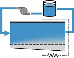
2. Problem formulation
In figure 1(a) a schematic illustration of a single-flow membraneless flow battery system is presented. Figure 1(b) focuses on the battery cell , which includes a main channel (region 1) bounded by upper and bottom electrodes. The bottom electrode is perforated, and allows flow to a secondary channel (region 2). We adopt the Cartesian system of coordinates,  $(x,\, y)$, as indicated in the figure, where the $x$ axis denotes the direction parallel to the bottom wall of region 1 and the $y$ axis is perpendicular thereto. The velocity of the fluid in these directions is denoted by $u=u(x,\, y)$ and $v=v(x,\, y)$, respectively. We here assume the battery operates at the dilute solution limit, which enables decoupling of the hydrodynamic and mass transfer problems. We hereafter denote dimensional variables by tildes, normalized variables without tildes and characteristic values by an asterisk superscript.

Figure 1. (a) Schematic illustration of a discharging single-flow membraneless flow battery system, which consists of the electrolyte storage tank, a pump and the active cell unit where the redox reaction takes place, bordered by the electrodes (red). (b) Schematic cross-sectional view of the cell, where the coordinate system and the key parameters used for the analysis are indicated. The permeable electrode, modelled as a thin porous plate, is marked by the dashed line delineating regions 1 and 2, alongside the 95 % mass transport boundary layer,  $\delta$ (dotted).
The length of the cell is denoted by  $L$. The line $y=0$ corresponds to the boundary between the two regions. The subscripts 1 and 2 denote variables and coordinates in regions 1 and 2, respectively. The floor of the channel in region 2 is assumed to be inclined relatively to the $x$-axis, and is defined by $\tilde {h}_2(\tilde {x}) = -H_{2} (1+S \tilde {x}/L)$, where S denotes the slope of the bottom wall and $H_{i}$ are the nominal heights of the channels.
We investigate slender channel geometries with aspect ratios  $H_{i}/L \ll 1$. The characteristic scales for length, channel height, mean downstream velocity and kinematic viscosity for such systems are given by $L \sim 0.1$ m, $H_{1} \sim 1\cdot 10^{-3}$ m, $u \sim 0.01$ m s $^{-1}$, $\nu =10^-{6}$ m $^2$ s $^{-1}$, respectively, where $\nu$ is the kinematic viscosity, and therefore the Reynolds reduced number for the system is Re $_{r}=$ $({H_{i}}/{L})({u H_{i}}/{\nu })\sim 0.1 \ll 1$, for which inertial effects are negligible.
Assuming Newtonian incompressible flow, the fluid motion, with a dynamic viscosity,  $\mu$, is governed by the Stokes equations representing conservation of momentum alongside conservation of mass. The governing fluid dynamic equations may be expressed as follows:
 $$\begin{align} \mu\left(\frac{\partial^{2}\tilde{u}_{i}}{\partial\tilde{x}^{2}} + \frac{\partial^{2}\tilde{u}_{i}}{\partial\tilde{y}_{i}^{2}}\right) &= \frac{\partial\tilde{p_{i}}}{\partial\tilde{x}}, \quad i = 1,2, \end{align}$$
 $$\begin{align}\mu\left(\frac{\partial^{2}\tilde{v}_{i}}{\partial\tilde{x}^{2}} + \frac{\partial^{2}\tilde{v}_{i}}{\partial\tilde{y}_{i}^{2}}\right) &= \frac{\partial\tilde{p}_{i}}{\partial\tilde{y}_{i}}, \quad i = 1,2, \end{align}$$
 $$\begin{align}\frac{\partial\tilde{u}_{i}}{\partial\tilde{x}} + \frac{\partial\tilde{v}_{i}}{\partial\tilde{y_{i}}} &= 0, \quad i = 1,2. \end{align}$$
These equations are subject to no-slip boundary conditions at the top and bottom walls of each region ( $\tilde {y}_{1}=H_{1},\, \tilde {y}_{i}=0$), as well as at the confining wall upstream the bottom region, i.e. $\tilde {y}_{2}=\tilde {h}_{2}$. In addition, a no-penetration boundary condition is imposed at the top and bottom walls of the cell. The pressure at the inlet and outlet is $p_{in}$ and $p_{out}$, respectively, and there is a no-flux boundary condition for the pressure at $\tilde {x}=0$ in the bottom region. To conclude this, the boundary conditions are given by
 \begin{equation} \left. \begin{array}{c} \tilde{u}_{1}|_{\tilde{y}_{1} = H_{1}} = \tilde{u}_{1}|_{\tilde{y}_{1} = 0} = 0, \quad \tilde{u}_{2}|_{\tilde{y}_{2} = 0} = \tilde{u}_{2}|_{\tilde{y}_{2} = \tilde{h}_2} = 0, \quad \tilde{p}_{1}|_{\tilde{x} = 0} = \tilde{p}_{in}, \quad \left.\dfrac{\partial\tilde{p}_{2}}{\partial\tilde{x}}\right|_{\tilde{x} = 0} = 0,\\ \tilde{v}_{1}|_{\tilde{y}_{1} = H_{1}} = 0, \quad \tilde{v}_{2}|_{\tilde{y}_{2} = \tilde{h}_2} = 0, \quad \tilde{p}_{1}|_{\tilde{x} = L} = \tilde{p}_{2}|_{\tilde{x} = L} = \tilde{p}_{out}. \end{array}\right\}\end{equation}
The average fluid flux across the bottom electrode is given by
 \begin{equation} \tilde{v}_{1}|_{\tilde{y}_1 = 0} = \tilde{v}_{2}|_{\tilde{y}_2 = 0} = \frac{k}{w\mu}(\tilde{p}_{2}|_{\tilde{y} = 0^{-}}- \tilde{p}_{1}|_{\tilde{y} = 0^{ + }}),\end{equation}
where  $k$ and $w$ are the permeability and the width of the bottom electrode, respectively, and $\tilde {p}_{i},\, i=1,\, 2$, is the pressure in the corresponding region.
In the next section the approach for obtaining an approximate solution for the problem in (2.1)–(2.3) is discussed.
3. Analysis
In this section we scale the governing equations and employ asymptotic expansions in order to obtain solutions of the flow and pressure fields up to first order.
3.1 Scaling
To rewrite the problem in dimensionless form, let us define the characteristic pressure and velocity parameters in each direction, which are assumed to be positive, as  $u_{i}^{*},\, v^{*}_{i},\, p^{*}>0$, where some restrictions and relations between the characteristic values will be discussed later in this section. Scaling by these characteristic values, we define the non-dimensional variables as follows:
 \begin{equation} (x,y_i) = \left(\frac{\tilde{x}}{L}, \frac{\tilde{y}_{i}}{H_{i}}\right), \quad (u_{i},v_i) = \left(\frac{\tilde{u}_{i}}{u_{i}^{ * }}, \frac{\tilde{v}_{i}}{v_{i}^{ * }}\right), \quad p_{i} = \frac{\tilde{p}_{i}-p_{out}}{p^{ * }}, \quad i = 1,2.\end{equation}
Next, let us define the slenderness ratios as
 \begin{equation} \varepsilon_{i} = \frac{H_{i}}{L}\ll1,\quad i = 1,2.\end{equation}
Substituting the scaled values and  $\varepsilon _{i}$ in (3.1a–c) and (3.2) into the governing equations in (2.1) and the boundary conditions in (2.3), results in the following set of the normalized governing equations:
 $$\begin{align} \frac{u_{i}^{ * }\mu}{L}\left(\varepsilon_{i}^{2} \frac{\partial^{2}u_{i}}{\partial x^{2}} + \frac{\partial^{2}u_{i}}{\partial y_{i}^{2}}\right) &= \varepsilon_{i}^{2}p^ * \frac{\partial p_{i}}{\partial x}, \quad i = 1,2, \end{align}$$
 $$\begin{align}\frac{u_{i}^{ * }\mu}{L}\left(\varepsilon_{i}^{2} \frac{\partial^{2}v_{i}}{\partial x^{2}} + \frac{\partial^{2}v_{i}}{\partial y_{i}^{2}}\right) &= p^ * \frac{\partial p_{i}}{\partial y_{i}}, \quad i = 1,2, \end{align}$$
 $$\begin{align}\varepsilon_{i}\frac{\partial u_{i}}{\partial x} + \frac{v_{i}^{ * }}{u_{i}^{ * }}\frac{\partial v_{i}}{\partial y_{i}} &= 0, \quad i = 1,2, \end{align}$$
as well as the boundary conditions at the separator between the two regions
 \begin{equation} v_{i}|_{y_i = 0} = \frac{k p^{ * }}{w\mu v_{i}^{ * }} (p_{2}|_{y = 0^{-}} - p_{1}|_{y = 0^{ + }} ), \quad i = 1,2.\end{equation}
 To obtain various relations between the characteristic values we employ the dominant balance approach for these equations. More specifically, let us first require that terms on both sides of (3.3c) for  $i=1,\, 2$ are of the same order of magnitude with respect to $\varepsilon _{i}$, respectively, yielding a relation for the velocities and the slenderness ratio
 \begin{equation} \frac{v_{i}^{ * }}{u_{i}^{ * }} = \varepsilon_{i}, \quad i = 1,2.\end{equation}
Next, by requiring that terms on both sides of the equation in (3.3a) for  $i=1,\, 2$ will be of the same order of magnitude with respect to $\varepsilon _{i}$, respectively, a pressure-dissipation scaling relation is obtained
 \begin{equation} u_{i}^{ * } = \frac{\varepsilon_{i}^{2}L p^{ * }}{\mu}, \quad i = 1,2. \end{equation}
Note that the expressions in (3.6) yield a velocity scaling between the two regions
 \begin{equation} \frac{u_{1}^{ * }}{u_{2}^{ * }} = \left(\frac{\varepsilon_{1}}{\varepsilon_{2}}\right)^{2}. \end{equation}
Substituting the expressions in (3.5) and (3.6) in (3.4), gives a relation for the pressure difference across the separator and the vertical velocities
 \begin{equation} v_{i}|_{y_i = 0} = K_{i}(p_{2}|_{y = 0^{-}}- p_{1}|_{y = 0^{ + }}), \quad i = 1,2, \end{equation}
where  $K_i$ denotes the dimensionless permeability parameters:
 \begin{equation} K_{i} = \frac{k}{wL\varepsilon_{i}^{3}} , \quad i = 1,2. \end{equation}
For brevity, let us further define  $K$ as the dimensionless permeability in region 1, namely $K=K_1$. Thus, $K_2$ satisfies $K_2=(H_1/H_2)^3\,K$.
Substituting the expressions obtained in (3.5), (3.8) and (3.9) into the governing equations (3.3) and the boundary conditions in (2.2) and (3.4) results in the following scaled governing equations:
 $$\begin{align} \varepsilon_i^2\frac{\partial^{2}u_{i}}{\partial x^{2}} + \frac{\partial^{2}u_{i}}{\partial y_{i}^{2}} &= \frac{\partial p_{i}}{\partial x}, \quad i = 1,2, \end{align}$$
 $$\begin{align}\varepsilon_{i}^{2}\left(\varepsilon_{i}^{2} \frac{\partial^{2}v_{i}}{\partial x^{2}} + \frac{\partial^{2}v_{i}}{\partial y_{i}^{2}}\right) &= \frac{\partial p_{i}}{\partial y_{i}}, \quad i = 1,2, \end{align}$$
 $$\begin{align}\frac{\partial u_{i}}{\partial x} + \frac{\partial v_{i}}{\partial y_{i}} &= 0, \quad i = 1,2, \end{align}$$
and the corresponding scaled boundary conditions
 \begin{equation} \left.\begin{array}{c} u_{1}|_{y_{1} = 1} = u_{1}|_{y_{1} = 0} = 0, \quad u_{2}|_{y_{2} = 0} = u_{2}|_{y_{2} = {-}(1 + S x)} = 0, \quad p_{1}|_{x = 0} = p_{in}, \quad \left.\dfrac{\partial p_{2}}{\partial x}\right|_{x = 0} = 0,\\ v_{1}|_{y_{1} = 1} = 0, \quad v_{2}|_{y_{2} = {-}(1 + S x)} = 0, \quad p_{1}|_{x = 1} = p_{2}|_{x = 1} = 0,\\ v_{i}|_{y_i = 0} = K_{i}(p_{2}|_{y = 0^{-}}- p_{1}|_{y = 0^{ + }}), \quad i = 1,2. \end{array} \right\} \end{equation}
 In this paper we concentrate only on the leading-order problems with respect to  $\varepsilon _{i},\, i=1,\, 2$, so that the terms of orders $\mathcal {O}(\varepsilon _i^2),\, i=1,\, 2$, are hereafter neglected. In the next section we will discuss our approach for asymptotic solution of this problem.
3.2 Asymptotics for the limit of small permeability
We focus on configurations where
 \begin{equation} 0< K\ll 1 \quad \text{and} \quad 0<\varepsilon_{2}<\varepsilon_{1}. \end{equation}
For common configurations, the order of magnitude of the characteristic values for the length, width and permeability of the bottom electrode are  $L,\, w \sim 10^{-2}\ \textrm {m},\, k \sim 10^{-10}\ \textrm {m}^2$, respectively. As for the slenderness ratio, the characteristic values are $\varepsilon _{1} \sim 10^{-1}$, therefore justifying (3.12a,b).
Hence, an asymptotic expansion with respect to  $K$ is well defined. Expanding the velocities and the pressures in regular asymptotic series with respect to the permeability parameter $K$, results in
 \begin{equation} \left. \begin{array}{c} u_{i}(x,y_{i}) = u_{i}^{(0)}(x,y_{i}) + K u_{i}^{(1)}(x,y_{i}) + \mathcal{O}(K^{2}), \quad i = 1,2,\\ v_{i}(x,y_{i}) = v_{i}^{(0)}(x,y_{i}) + K v_{i}^{(1)}(x,y_{i}) + \mathcal{O}(K^{2}), \quad i = 1,2,\\ p_{i}(x,y_{i}) = p_{i}^{(0)}(x,y_{i}) + K p_{i}^{(1)}(x,y_{i}) + \mathcal{O}(K^{2}), \quad i = 1,2,\end{array}\right\} \end{equation}
where the superscript indicates the order, zero denoting the leading order and one denoting the first order.
Our approach to this problem is outlined as follows. In § 3.2.1 we obtain the leading-order solution with respect to  $K$ in region 1. We then use it to obtain the leading-order solution in region 2. Both leading-order solutions are then employed in § 3.2.2 in order to get the first-order solution with respect to $K$ in region 1. Note that this procedure may be continued in the same manner, thus allowing us to obtain the solutions to the problems in regions 1 and 2, up to any desired order.
3.2.1 Leading-order solution with respect to permeability parameter in regions 1 and 2
Let us start with the leading-order problems. Substituting the expansions in (3.13) into the equations and the boundary conditions in (3.10) and (3.11), we get that the leading-order equations with respect to  $K$ in regions 1 and 2, respectively, are given by
 $$\begin{align} \frac{\partial^{2}u_{i}^{(0)}}{\partial y_{i}^{2}} &= \frac{\partial p_{i}^{(0)}}{\partial x}, \quad i = 1,2, \end{align}$$
 $$\begin{align}\frac{\partial p_{i}^{(0)}}{\partial y_{i}} &= 0, \quad i = 1,2, \end{align}$$
 $$\begin{align}\frac{\partial u_{i}^{(0)}}{\partial x} + \frac{\partial v_{i}^{(0)}}{\partial y_{i}} &= 0, \quad i = 1,2. \end{align}$$
In region 1, (3.14) are solved subject to the corresponding boundary conditions
 \begin{equation} u_{1}^{(0)}|_{y_{1} = 1} = u_{1}^{(0)}|_{y_{1} = 0} = 0 , \quad v_{1}^{(0)}|_{y_{1} = 1} = v_{1}^{(0)}|_{y_{1} = 0} = 0 , \quad p_{1}^{(0)}|_{x = 0} = p_{in} , \quad p_{1}^{(0)}|_{x = 1} = 0. \end{equation}
It is easy to verify that the solution for this problem may be expressed as
 \begin{equation} u_{1}^{(0)}(x,y_1) = \frac{p_{in}}{2}(y_{1}-y_{1}^{2}), \quad v_{1}^{(0)}(x,y_1) = 0 , \quad p_{1}^{(0)}(x,y_1) = p_{in}(1-x).\end{equation}
Note that, according to the solution, as shown in (3.16a–c), for the leading-order problem in region 1, there is no mass transport to the lower region. As a result, the velocity is a Poiseuille flow velocity profile, as expected for a channel flow.
Next, let us solve the leading-order problem in region 2 given in (3.14), which is solved subject to the following boundary conditions:
 \begin{equation} \left. \begin{array}{c} u_{2}^{(0)}|_{y_{2} = 0} = u_{2}^{(0)}|_{y_{2} = {-}(1 + S x)} = 0 , \quad v^{(0)}_{2}|_{y_{2} = {-}(1 + S x)} = 0 , \quad p_{2}^{(0)}|_{x = 1} = 0 , \quad \left.\dfrac{\partial p_{2}^{(0)}}{\partial x}\right|_{x = 0} = 0, \\ v_{2}^{(0)}|_{y_2 = 0} = \left(\dfrac{H_1}{H_2}\right)^3\,K (p_{2}^{(0)}|_{y = 0^{-}}-p_{1}^{(0)}|_{y = 0^{ + }}), \end{array}\right\}\end{equation}
where the last boundary condition in (3.17) is not homogeneous, since  $(H_1/H_2)^3\,K$ is of order $\mathcal {O}(1)$ with respect to $K$, but not $\mathcal {O}(K)$. In the same manner as for the leading-order problem in region 1, by looking at (3.14b), one can see that in the bottom region the pressure is constant at each cross-section along the channel, i.e. ${p_{2}^{(0)}(x,\, y_2)=}p_{2}^{(0)}(x)$, which simplifies the equations. Next, solving (3.14a) subject to the no-slip boundary conditions at the top and bottom walls of region 2, gives
 \begin{equation} u_{2}^{(0)}(x,y_2) = \frac{y_{2}}{2}\frac{\partial p_{2}^{(0)}}{\partial x} (1 + Sx + y_{2}).\end{equation}
Substituting equation (3.18) into the governing equation for the mass conservation equation in (3.14c), yields
 \begin{equation} \frac{y_{2}}{2}\left(S\frac{\partial p_{2}^{(0)}}{\partial x} + \frac{\partial^{2}p_{2}^{(0)}}{\partial x^{2}}(1 + Sx + y_{2})\right) + \frac{\partial v_{2}^{(0)}}{\partial y_{2}} = 0.\end{equation}
Solving this equation subject to the no-penetration boundary condition at the top of the channel results in the following expression for  $v_{2}^{(0)}(x,\, y_2)$:
 \begin{equation} v_{2}^{(0)}(x,y_2) = \frac{1}{12}\left(3S\frac{\partial p_{2}^{(0)}}{\partial x} ((1 + Sx)^{2}-y_{2}^{2}) + \frac{\partial^{2}p_{2}^{(0)}}{\partial x^{2}} ((1 + Sx-2y_{2})(1 + Sx + y_{2})^{2})\right). \end{equation}
Imposing on (3.20) the corresponding boundary condition in (3.17) at  $y_2=0$, gives
 \begin{equation} \frac{\partial^{2}p_{2}^{(0)}}{\partial x^{2}}(1 + Sx)^3 + 3S\frac{\partial p_{2}^{(0)}}{\partial x}(1 + Sx)^{2} = 12(H_1/H_2)^3\,K (p_{2}^{(0)}-p_{1}^{(0)}), \end{equation}
where we have used the independence of the pressures,  $p_{1}^{(0)}(x)$ and $p_{2}^{(0)}(x)$, of $y_1$ and $y_2$, respectively.
Forming an asymptotic expansion with respect to the inclination parameter,  $|S| \ll 1$ gives
 \begin{equation} p_{2}^{(0)}(x) = p_{2}^{(0,0)}(x) + Sp_{2}^{(0,1)}(x) + \mathcal{O}(S^2),\end{equation}
where the second superscript index indicates the order of the term with respect to  $S$, with zero denoting the leading-order term. For further detail regarding the asymptotic approximation with respect to the inclination parameter see Appendix A.
In (3.22)
 \begin{equation} p_{2}^{(0,0)}(x) = \frac{p_{in}}{6(1 + e^{4Z})} \left(6-\frac{3}{Z}(e^{{-}2Z(x-2)}-e^{2Zx})-6e^{4Z} (x-1)-6x\right),\end{equation}
and
 \begin{align} p_{2}^{(0,1)}(x)& = {-}\frac{e^{2Z(2-3x)}p_{in}}{16(1 + e^{4Z})^{2}(H_1/H_2)^3K} \{8e^{6 Zx}-4e^{2Z(2x-1)}-4e^{2Z(2x + 1)} + 4e^{2Z(3x-2)} + 4e^{2Z(3x + 2)}\nonumber\\ &\quad -4e^{2Z(4x-1)}-4e^{2Z(4x + 1)} + e^{4Z(x + 1)}[12(H_1/H_2)^3\,K x^2-2Zx-1]\nonumber\\ &\quad + e^{4Z(2x-1)}[12(H_1/H_2)^3Kx^2 + 2Zx-1]\nonumber\\ &\quad + e^{4Zx}[1-2Zx + 12(H_1/H_2)^3K(x^2-2)] + e^{8Zx}[1 + 2Zx + 12(H_1/H_2)^3K(x^2-2)]\}, \end{align}
where we have defined for brevity,  $Z=\sqrt {3(H_1/H_2)^3K}$. Using this result in (3.18) and (3.20), we obtain the approximate (up through order $\mathcal {O}(S^2)$) velocities $u_{2}^{(0)}(x,\, y_2)$ and $v_{2}^{(0)}(x,\, y_2)$ in region 2.
3.2.2 First-order solution with respect to permeability parameter in region 1
Now, after we have found the leading-order solutions with respect to the permeability parameter,  $K$, in regions 1 and 2, let us solve the first-order problem in region 1. The first-order problem is composed of the following equations:
 $$\begin{align} \frac{\partial^{2}u_{1}^{(1)}}{\partial y_{1}^{2}} &= \frac{\partial p_{1}^{(1)}}{\partial x}, \end{align}$$
 $$\begin{align}\frac{\partial p_{1}^{(1)}}{\partial y_{1}}& = 0, \end{align}$$
 $$\begin{align}\frac{\partial u_{1}^{(1)}}{\partial x} + \frac{\partial v_{1}^{(1)}}{\partial y_{1}} &= 0, \end{align}$$
which are subject to the boundary conditions
 \begin{equation} \left. \begin{array}{c} u_{1}^{(1)}|_{y_{1} = 1} = u_{1}^{(1)}|_{y_{1} = 0} = 0 , \quad v_{1}^{(1)}|_{y_{1} = 1} = 0 , \quad p_{1}^{(1)}|_{x = 0} = 0 , \quad p_{1}^{(1)}|_{x = 1} = 0\\ v_{1}^{(1)}|_{y_1 = 0} = (p_{1}^{(0)}-p_{2}^{(0)}) \end{array}\right\}, \end{equation}
where  $p_{1}^{(0)}(x)$ and an approximation for $p_{2}^{(0)}(x)$, up through order $\mathcal {O}(S^2)$, are known from the previous section.
As previously, solving the downstream momentum equation (3.25a) subject to the no-slip boundary conditions at both walls gives
 \begin{equation} u_{1}^{(1)}(x,y_1) = \frac{y_{1}}{2}\frac{\partial p_{1}^{(1)}}{\partial x}(y_{1}-1). \end{equation}
Next, using (3.27) in the mass conservation equation (3.25c), and the no-penetration boundary condition at the top wall of region 1 yields
 \begin{equation} v_{1}^{(1)}(x,y_1) = \frac{1}{12}\frac{\partial^{2}p_{1}^{(1)}}{\partial x^{2}}({-}2y_{1}^{3} + 3y_{1}^{2}-1). \end{equation}
 Finally, substituting equation (3.28) in (3.26) as well as the expressions for  $p_1^{(0)}(x)$ and $p_2^{(0)}(x)$, which are given in (3.16a–c) and (3.22), respectively, we may obtain, by solving the resulting second-order ordinary differential equation (ODE), the expression for pressure $p_{1}^{(1)}(x)$.
4. Results and discussion
4.1 Flow field and numerical validation
Let us first present the obtained flow field for two configurations with the inclinations of  $S=0$ and $0.5$ and a dimensionless permeability of $K=k w L \varepsilon _1^2=0.1$, where $H_2/H_1=1/5$ and $H_1/L=1/10$. The flow fields are presented in figure 2. There is a good agreement between the analytic and numerical results, thus verifying our asymptotic approximation. The effect of the inclination of the bottom wall on the velocity near the bottom electrode is evident here, and velocity in the $y$-direction does not vanish for $S\neq 0$ in the bottom region. To further focus on the effect of the bottom channel, we visualize the change of the velocity field in the following figures. For details regarding the numerical scheme, see Appendix B; for a quantitative assessment of the accuracy of the analytical model see Appendix C.

Figure 2. The flow field in the cell represented by streamlines obtained analytically (blue, solid) alongside numerical computations (black, dotted) for  $K=k/w L \varepsilon _1^2=0.1,\, H_1/H_2=1/5$ and $H_1/L=10$, and for (a) $S=0$ and (b) $S=0.5$.
4.2 Permeability and inclination effects on the pressure distribution
Figures 3(a) and 3(b) present the pressure distribution in the upper and lower channels as a function of electrode permeability and inclination of the bottom wall. Figure 3(a) shows that, with increasing permeability, the pressures at the bottom channel and at the top channel achieve synchronization closer to the inlet. Figure 3(b) illustrates the effect of channel slope  $S$, which for $S\neq 0$ prevents full synchronization of the pressures at the main and adjacent channels. Figures 3(c) and 3(d) present the correction to the pressure at the main channel, $p_1^{(1)}$. Figure 3(c) examines the effect of the slope of the bottom wall, $S$, and figure 3(d) illustrates the effect the channel height ratio, $H_2/H_1$. The results indicate that the pressure correction is negative throughout the channel for $S\geq 0$. This reduction of the pressure at the top channel is a result of fluid transfer to the bottom channel, which in turn reduces flux in the upper channel. For the inclination of $S=-0.25$ a transition from negative to positive pressure can be observed. Reducing the value of the ratio $H_2/H_1$ increases the effect of the bottom channel and shifts the location of the maximum of $p_1^{(1)}$ towards the outlet.

Figure 3. The pressure at the top channel (dashed red),  $p_{1}$, and the pressure at the bottom channel for (a) various permeability values and $S=0$ and (b) for different slopes and $K=0.1$. In (c) and (d), the first-order asymptotic correction at the top channel, $p_1^{(1)}$, due to the adjacent channel is shown for $K=0.1$ and for (c) $H_2/H_1=1/5$ and different inclination values, $S$, including the case without any inclination (marked in red) and (d) $S=-0.5$ and different channel thicknesses ratios, $H_2/H_1$. The pressure at the top channel is given by $p=(p_{in}-p_{out})(1-x)+K p^{(1)}_1$, and it is independent of the $y$ coordinate.
4.3 Flow through the bottom electrode
While having only a small effect on the speed in the streamwise direction, the bottom channel is the only cause of flow in the direction perpendicular to the bottom electrode,  $v_{1}=v^{0}_{1}+K v^{1}_{1}$, which is crucial to the efficiency of flow batteries. Figure 4 depicts the velocity in the $y$-direction in the upper channel $v_{1}^{(1)}$ for various configurations, where negative values represent velocity towards the bottom region. For parallel channels, $S=0$, the downward flow is fastest for $x\rightarrow 0$ and decreases with increasing $x$ until it reaches a plateau of $v_1(y=0)=v_2(y=0)\rightarrow 0$, i.e. no mass transport between the regions, as shown in figure 4(a,b). The balance in mass transport can be attributed to the pressure synchronization of the two channels. For higher permeability values, $v_{1}^{(1)}=0$ is reached for a smaller $x$ due to a higher mass transport between the regions. For an expanding channel, $S=0.5$, the flow throughout the electrode is negative, and decreases in amplitude with increasing $x$, as presented in figure 4(c). For $S=-0.5$, the value of $v_{1}^{(1)}$ is negative similarly to other $S$ values, but it changes sign at $x\approx 0.175$, indicating a flow from the bottom to the top channel, as depicted in figure 4(d).

Figure 4. The first-order term in the asymptotic expansion of the vertical velocity with respect to  $K,\, v_1^{(1)}$, which is calculated as the sum of two first terms in the expansion with respect to $S$, versus $x$ at the top channel (region 1), visualizing the effect of the adjacent channel (region 2) for (a) and (b) parallel channels, $S=0$, with $K=0.01$ and $K=0.1$, respectively, and for (c) and (d) tapered bottom channel with $K=0.1$, where the slope of the channel in (c) and (d) is $S=0.5$ and $S=-0.5$, respectively. Positive and negative values of $v_1^{(1)}$ correspond to downward and upward velocity of the fluid, respectively.
4.4 Induced flow field and reactant boundary layer
In figure 5 we show the analytically calculated first order of the asymptotic expansion of the velocity with respect to  $K$ (see equations, (3.27) and (3.28)), created due to the adjacent channel. Overlaid behind the streamlines are the concentration profiles of a neutrally charged reactant which enters the main channel, and which reacts at the permeable electrode. A detailed description of the calculations can be found in the following section. Different columns in figure 5 correspond to different values of the slope $S$ and the different rows correspond to different values of electrode permeability $K$.
$K$.

Figure 5. The flow field in the cell where only the first order of the asymptotic expansion of the velocity with respect to  $K$ in the top channel, $(u^{(1)}_{1},\, v^{(1)}_{1})$, is presented along the total flow field in the bottom channel $(u_{2},\, v_{2})$. The flow fields are given for $H_1/H_2=1/5$ and for different permeability and slope values. The orange regions represent normalized concentration of the electrolyte with scaled $y$-values, which are shown on the right axis of the figure. The rows (top to bottom) stand for $K=0.01,\, 0.1,\, 0.35$, and the columns (left to right) represent $S=-0.5,\, 0,\, 0.5$.
Flow fields with same slope value,  $S$, exhibit similar characteristics, as shown in each column in figure 5. For all slopes there is a focusing of the streamlines at a specific location directed towards the bottom channel, occurring due to a change in the $x$-direction component of the velocity field. The location of this focus point is shifted towards the outlet as $S$ increases. For the non-negative slopes ( $S=0,\, 0.5$), the $y$-component of the velocity field is negative or zero throughout the main channel. In contrast, for the negative slope ( $S=-0.5$) the value of the $y$-component of the velocity field becomes positive between the focusing point and the outlet. Moreover, for these cases, the flow in the major part of the electrode is from the bottom channel to the main channel due to narrowing of the bottom channel to satisfy mass conservation. For parallel channels, $S=0$, in most of the electrode there is no mass transport to the bottom channel. For such configurations, the velocity field in the bottom channel becomes parallel to the $x$-axis. This phenomenon is observed only in the case of zero slope.
Next, let us discuss the impact of the permeability parameter,  $K$. For non-positive values of $S$, a higher permeability shifts the position of the focusing point of the streamlines, directed towards the bottom channel, towards the inlet and for negative $S$ also that of the upper stream. On the contrary, for the positive value of $S$, we observe the opposite trend, and for increasing $K$ the location of the focus point of the flow to the bottom channel is shifted towards the outlet. Moreover, for $S=0$ increasing $K$ causes a reduction of the surface area through which the mass transport from the top channel to the bottom channel occurs.
4.5 Battery limiting current
We here consider a neutrally charged reactant present in the flow, as well as a dilute electrolyte. Neutrally charged reactants can represent halides, for example bromine in a zinc–bromine (Reference Braff, Buie and BazantBraff, Buie, & Bazant, 2013; Reference Mader and WhiteMader & White, 1986; Reference Ronen, Gat, Bazant and SussRonen et al., 2021), quinone–bromine (Reference Chen, Gerhardt and AzizChen, Gerhardt, & Aziz, 2017) or hydrogen–bromine flow battery (Reference Cho, Albertus, Battaglia, Kojic, Srinivasan and WeberCho et al., 2013; Reference Ronen, Atlas and SussRonen, Atlas, & Suss, 2018). For such batteries, when using a planar bromine electrode and discharging the battery, the structure of the bromine boundary layer forming along the electrode determines the maximum bromine flux to the electrode, and so the battery's limiting (maximum) current (Reference Braff, Buie and BazantBraff et al., 2013; Reference Ronen, Gat, Bazant and SussRonen et al., 2021). For this reason, strategies which compress the bromine boundary layer, such as increasing the electrolyte flow rate, can improve the battery limiting current and reduce voltage losses for high current operation. We here consider a perforated planar electrode between the two flow channels, as highly conductive planar electrodes are often used in membraneless cells, largely due to the challenge in compressing adequately a porous electrode in cells with open channels (Reference Braff, Buie and BazantBraff et al., 2013; Reference Suss, Conforti, Gilson, Buie and BazantSuss, Conforti, Gilson, Buie, & Bazant, 2016). As described in previous works, the boundary layer along a planar bromine electrode can be determined by solving the following balance equation for a neutrally charged reactant in a flowing, dilute electrolyte solution (Reference Braff, Buie and BazantBraff et al., 2013; Reference Ronen, Gat, Bazant and SussRonen et al., 2021),
 \begin{equation} D \nabla^2 c + \boldsymbol{\nabla} \boldsymbol{\cdot} (\boldsymbol{u}c) = 0,\end{equation}
where  $D$ is the reactant species diffusion coefficient, $c$ is the concentration and $\bar {u}$ is the velocity vector. Variables are non-dimensionalized according to (2.2) with the addition of the normalized concentration $c=\tilde {c}/c_0$.
In order to explore the effect of the flow field and adjacent channel geometry on battery current capability, we solve (4.1) at the limiting current, where the reactant is entirely depleted along the permeable electrode during discharge. At the inlet and along the porous electrode plate, we impose fixed concentration (Reference Braff, Buie and BazantBraff et al., 2013),
 \begin{equation} c|_{{x = 0}} = 1, \quad c|_{y_{1} = 0} = 0.\end{equation}
 Assuming an impermeable anode and high Péclet number,  $Pe$=
$Pe$= $UH_1$/ $D$, and where $U$ is the mean axial velocity, allows us to write
 \begin{equation} \boldsymbol{\nabla} c|_{x = 1}\boldsymbol{\cdot} \hat{n} = \boldsymbol{\nabla} c|_{y_1 = 1} \boldsymbol{\cdot} \hat{n} = 0,\end{equation}
where  $\hat {n}$ is the surface normal vector. Equation (4.1) with the boundary conditions in (4.2a,b) and (4.3) was solved using COMSOL Multiphysics 5.4 software.
At the limiting current, the reactant flux to the cathode is maximized and given by  $N_w=({DC_0}/{H_1})({\partial c}/{\partial y_1})\rvert _{y_1=0}$, where, $c_0$ is unity. The current density, $J$, can be related to flux by multiplying flux by $nF$, where $n$ is the number of electrons per reactant molecule participating in the electrochemical reaction, and $F$ is Faraday's constant. By applying Faraday's law to obtain the current density at the electrode, $J$, and defining the dimensionless local current density as $J=H_1j/nDFc_0$, we obtain $J_{lim}={\partial c}/{\partial y_1}\rvert _{y_1=0}$.
For the reference case of zero flow through the electrode,  $K=0$, our numerical model for limiting current was benchmarked to the analytical solution provided by Reference Braff, Buie and BazantBraff et al. (Reference Braff, Buie and Bazant2013). The latter solution is for the limiting current in a planar electrode cell with a thin concentration boundary layer of a neutrally charged reactant and linearized Poiseuille flow.
In figure 5, we presented the predicted concentration boundary layer of a neutrally charged reactant along the permeable electrode, in addition to the flow streamlines for  $H_2/H_1=1/5$, various electrode permeabilities and bottom channel inclinations. The boundary layer thickness is affected by the bottom channel slope, $S$, as illustrated in figure 5. As the slope increases, the concentration boundary layer becomes thinner, resulting in faster diffusive reactant transport to the electrode, thus enhancing its performance. For instance, for $K = 0.01$ and $S=-0.5$, the boundary layer becomes fully developed by $x=1$, whereas for $S=0.5$ it is still developing.
The predicted non-dimensional current density,  $J$, for a battery discharging at the limiting condition is presented in figure 6 alongside the averaged current in the inset, calculated by integrating local currents from $x = 0$ to $x$. The limiting conditions refer to the maximum possible discharge current, where the reactant concentration at the surface is zero. Figure 6(a) shows the effect of varying electrode permeability for a constant inclination, $S = 0.5$, compared with the reference configuration without a bottom channel, i.e. with an impermeable bottom electrode $K=0$. In all cases, the local current, affected by the growth of the concentration boundary layer, decreases rapidly along the channel length. Ultimately, we predict that, for $S = 0.5$, a permeable electrode outperforms the reference configuration without an adjacent channel, for all values of permeability tested here. We also investigated the effect of permeability, finding the accumulated current the electrode is $5\,\%$ lower for $K = 0.01$ than for $K = 0.1$ and $K = 0.35$, for which the current is practically identical. Figure 6(a) illustrates that, at low permeabilities, the cumulative current through the permeable electrode is slightly lower than at higher permeabilities, and at high permeability, the flow is mainly restricted to the entrance region.

Figure 6. Exploring the current density at the electrode for various configurations. (a) Local current along the channel for inclination  $S=0.5$ and varying permeability $K=0.01,\, 0.1$ and $0.35$. The inset shows the cumulative current with $x$, which is significantly improved with a permeable electrode, but is only slightly affected by permeability. (b) Local current for permeability $K=0.1$ and varying inclinations, $S= -0.5,\, 0$ and $0.5$. Inset shows cumulative current at the electrode up to $x$, where a positive inclination induces a twofold higher flux than a negative inclination.
In figure 6(b), we examine the current density for varying inclinations of the bottom channel,  $S$, at constant electrode permeability, $K = 0.1$. It shows that, throughout the channel, the current obtained increases with inclination $S$. At $x \geq 0.4$, the current is slightly lower for inclination $S = -0.5$ than for an impermeable electrode, $K = 0$. For the same combination of permeability and slope, figure 4(d) shows that, for $x \geq 0.15$, the vertical velocity in the upper channel becomes positive, so that the advective flux is away from the electrode. There is an offset between the of the $x$ location of the turn of the velocity direction with respect to the current. Thus, the entire length of the channel is not used efficiently in the case of $S = -0.5$. The inset of figure 6(b) shows that adding a second channel increases the reactant transport when compared with the classic configuration of a single channel. In particular, adding a parallel channel increases the reactant transport to 140 % of the reference case, whereas the highest averaged current is obtained for positive inclination $S=0.5$, resulting in an average current increase of 350 % over the case with no bottom channel, which is due in part to the thinner concentration boundary layer for this case, as seen in figure 5.
5. Conclusions
In this work, we analyse modifications of the flow field to the concentration boundary layer of a neutrally charged reactant forming along single-flow membraneless RFB electrode, aiming to improve such devices’ operation. Specifically, we model the effect of permeability of the perforated electrode and the geometry of the adjacent channel.
Our results indicate that mass transport through the bottom electrode is maximal near the inlet, and drops gradually. If the adjacent channel is of uniform thickness, the pressure fields in the main and the adjacent channels synchronize, and the flow through the bottom electrode vanishes. The channel length required to achieve synchronization decreases with increasing bottom electrode permeability. An adjacent channel with gradually changing thickness prevents synchronization of the pressures, leading to a more uniform flow through the bottom electrode. This, in turn, creates a more uniform boundary layer, and thus more effective reactant transport and distribution of the electrolytes over the porous electrode surface. The flow field in both channels can be designed to achieve a desired mass transport through the perforated electrode. Nevertheless, the effect on the flow field decreases with increasing the thickness ratio of the adjacent channel to the main channel.
For system optimization, results show that, for improved discharge performance, the highest mass transport to the permeable electrode serving as a cathode can be obtained by using scaled slope  $S = 0.5$ and scaled electrode permeability $K = 0.1$, while improved coulombic efficiency can be achieved by using $K = 0.01$ and $S = -0.5$. Future effort can extend the model provided here to the case of charged reactant species or a three-dimensional porous permeable electrode between the two channels. Overall, this theory provides an insight into the important role of flow physics on this promising sub-class of flow batteries and will help to pave the way to create more efficient flow batteries with minimal balance of plant.

Figure 7. The magnitude of the  $v$ component of the velocity field (a,b) analytically calculated, $|v_{analytical}|$, and (c,d) shown as the difference between the analytical and numerical calculations, $|v_{analytical}-v_{numerical}|$ for (a,c) a parallel channel, $S=0$, and (b,d) a slanted channel, $S=0.5$.
Supplementary material
Supplementary material are available at https://doi.org/10.1017/flo.2022.4. A Wolfram Mathematica file containing the derivation of the solution in its dimensional form presented in this paper is provided as part of the supplementary material.
Declaration of interests
The authors report no conflict of interest.
Funding
This study is Supported by The Nancy and Stephen Grand Technion Energy Program (GTEP), and the Ministry of National Infrastructures, Energy and Water Resources via graduate student scholarships in the energy fields.
Data availability statement
All other data included in the manuscript and/or supplemental materials are available from the corresponding authors upon request.
Ethical standards
The research meets all ethical guidelines, including adherence to the legal requirements of the study country.
Author contributions
A.G., M.S. and S.K. conceived the research. R.R. and Y.M. carried out the simulations. S.K. and A.G. conducted the theoretical analysis. S.K., A.G. and M.S. contributed to the interpretation of the results. S.K. took the lead in writing the manuscript. All authors provided critical feedback and helped shape the research, analysis and manuscript. All authors approved the final submitted draft.
Appendix A. Asymptotic scheme with respect to the inclination parameter
Let us consider the (3.21), which holds for  $p_{2}^{(0)}$. Note, that since $p_{2}^{(0)}$ is independent of $y_2$, (3.21) should be satisfied for all $y_2\in (-(1+S x),\, 0)$ and all $x\in (0,\, 1)$. Hence, substituting the solution for $p_1^{(0)}(x)$ which was given in (3.16a–c), we get that $p_2^{(0)}(x)$ should satisfy the following ODE:
 \begin{equation} \frac{\partial^{2}p_{2}^{(0)}}{\partial x^{2}} + \frac{3S}{(1 + Sx)} \frac{\partial p_{2}^{(0)}}{\partial x}-\frac{12(H_1/H_2)^3K}{(1 + Sx)^3}p^{(0)}_{2} = \frac{12(H_1/H_2)^3Kp_{in}(x-1)}{(1 + Sx)^3},\end{equation}
which should be solved subject to the boundary conditions
 \begin{equation} \left.\frac{\partial p_{2}^{(0)}}{\partial x}\right|_{x = 0} = 0, \quad p_{2}^{(0)}|_{x = 1} = 0. \end{equation}
 Since by our assumption the inclination parameter,  $S$, satisfies $|S| \ll 1$, in order to calculate the pressure and the resulting velocities analytically, we assume an asymptotic expansion of $p_{2}^{(0)}(x)$ with respect to the inclination parameter, $S$, namely we use the expansion in (3.22), Substituting this expansion into (A1), the resulting leading-order term satisfies
 \begin{equation} \frac{\partial^{2}p_{2}^{(0,0)}}{\partial x^{2}}-12(H_1/H_2)^3Kp_{2}^{(0,0)} = 12(H_1/H_2)^3Kp_{in}(x-1). \end{equation}
It is easy to verify that the solution for this equation subject to the boundary conditions (A2a,b) is given by the expression (3.23).
Next, let us solve the first-order problem, with respect to  $S$, resulting from (A1) subject to the boundary conditions given in (A2a,b), namely
 \begin{equation} \left. \begin{array}{c} \dfrac{\partial^{2}p_{2}^{(0,1)}}{\partial x^{2}}-12(H_1/H_2)^3Kp_{2}^{(0,1)} = {-}3\dfrac{\partial p_2^{(0,0)}}{\partial x}-36(H_1/H_2)^3Kx[p_{in}(x-1) + p_{2}^{(0,0)}],\\ \left.\dfrac{\partial p_{2}^{(0,1)}}{\partial x}\right|_{x = 0} = 0, \quad p_{2}^{(0,1)}|_{x = 1} = 0. \end{array} \right\}\end{equation}
It can be verified that the solution for this problem may be expressed as given in (3.24).
Appendix B. Flow field validation via numerical computations
Evaluation the theoretical model predictions for a straight and sloped channel was performed using COMSOL 5.5 (COMSOL, Inc., Burlington, MA, USA) 2D Free and Porous Media Flow (fp) module. We assume a Newtonian and incompressible flow with density  $\rho =1000$ kg m $^{-3}$, dynamic viscosity $\mu =0.0001 \textrm {Pa} \cdot \textrm {s}$ and fully saturated porous media. We uphold continuity with the Stokes–Brinkman formulation for both upper and lower fluid domains with a thin porous membrane, having permeability $K=0.001$ $\textrm {m}^{2}$, separating the two domains along their entire length. Using this more generalized formulation, we account for viscous transport (i.e. shear effects along walls not represented in the Darcy flow formulation) on both sides of a thin membrane so as to permit both qualitative and quantitative testing of our theoretical model.
The fluid domain consists of two flow channels. The upper channel having length and height  $L_1=0.1$ m and $H_1=0.01$ m, respectively, and a lower channel of the same length $L_1=L_2$ and of height $H_2 (x=0)=H_2 (x=L)=0.002$ m, for the straight channel case, and $H_2 (x=0)=0.002$ m and $H_2 (x=L)=0.00315$ m for the case of an $S=0.5$ inclined channel. A thin membrane $h_{membrane}=O(\varepsilon )=0.1$ mm separates the upper flow channel and the lower channels along their entire length. The upper channel has an extended inlet section spanning $-0.01\leq x \leq 0$ to allow for the fully developed flow profile at the inlet of the channel starting at $x \geq 0$ (see details below). The formulation of the finite element method model is complete by setting the boundary conditions at the inlet for the velocity $u(-0.01,\, y,\, t)={((\Delta P/\Delta x)/(2\mu ))y(H_1-y),\, 0}$ m s $^{-1}$, and the pressure, $\Delta P/\Delta x=1$ Pa m $^{-1}$ as unit pressure per unit length. As well as the pressure at upper and lower channel outlet, $p(0.1,\, y,\, t) =0$ Pa, and a no-slip condition to all external fluid domain walls. Last, we set a quiescent flow $u(x,\, y,\, 0)=0,\, p(x,\, y,\, t=0)=0$ as the initial condition for the entire fluid domain.
Our discretization consists of linear Lagrange elements in the fluid and porous media domains, and our mesh consists of  $O(2 \times 10^4)$ domain elements and $O(1 \times 10^3)$ quad boundary elements along wetted walls surfaces, corresponding to a total of $O(6 \times 10^4)$ degrees of freedom solved for.
Appendix C. Validity range of the flow model
To assess the quantitative accuracy of the model a comparison between the analytical and numerical flow fields is used. Since the flow fields of the velocity component parallel to the channel,  $u$, are very similar in both the analytical and numerical calculations, only the vertical component of the velocity fields, $v$, is further discussed. Figures 7(a) and 7(b) illustrate the analytically calculated $|v|$ component of the flow field where figure 7(c,d) shows the difference between the analytically and numerically obtained values $|v_{analytical}-v_{numerical}|$. We show the results for two slopes of the bottom channel wall $S=0$ and $S=0.5$, to be consistent with the parameters chosen in figure 2. In both cases, the differences are an order of magnitude smaller than the values of the velocity, and most of the difference is concentrated in a small region near the inlet between the channels, probably due to transition to Poiseuille flow. Accordingly, for systems meeting the assumptions of the model, the analytical derivation shown in this work can be used to obtain a good flow field approximation.
Next, let us address the range of values for which our analysis holds. Using scaling analysis we derive meaningful non-dimensional parameters that allow us to assess the relation between competing effects:
(i) Parameter $K={k}/{wL\varepsilon _{1}^{3}}>0$ describes the ratio of the electrode permeability to an equivalent permeability for flow in the upper channel. For $K\rightarrow 0$ there is no flow of the electrolyte through the bottom electrode and it therefore reduces the case to the classical design of a single channel battery. For $K>1$, most of the electrolyte flow downwards to the bottom channel. Both described cases are not of interest in this study. For the asymptomatic scheme, we also require $K\ll 1$. In figure 2 we therefore chose to present verification of the flow fields for $K=0.1$, which was chosen arbitrarily in the described range.
(ii) The parameter
$S$ describes the slope of the bottom channel bottom wall. To be able to calculate analytically the pressure in the bottom channel, and the induced flow and pressure fields in the top channel, we formed an asymptotic expansion with respect to this inclination parameter (described in (3.22)) and therefore we require $|S|\ll 1$. On the other limit, for $S\gg 1$ the bottom channel would act as an infinite drain, and mass transport from the bottom channel back to the top channel would not occur. On the other hand, since $\tilde {h}_2(\tilde {x}) = -H_{2} (1+S \tilde {x}/L)$ (shown in figure 1 and mentioned in § 2), and subsequently $h_{2}(x) = -H_{2} (1+S x)$, for $h_{2}(x)>0\rightarrow S>-1$, or else the system would be different, i.e. the bottom channel would have the same length of the top channel $L$, the boundary condition of $P_{out}$ at the bottom channel outlet would be irrelevant and all the electrolyte that would reach the bottom channel would have to be pushed out to the top channel eventually. The mentioned requirements define the range of relevant $S$ values. Within this range, we chose arbitrarily the value of $S=\pm 0.5$ as the largest value which still fits the mentioned above constraints, to show and investigate the effects of the slope on the flow fields.


To conclude, non-dimensional parameters allow us to express the range within which different physical effects are dominant. We chose values within the relevant ranges of interest to verify our analytical model by numerical solutions. We suggest that any other value within the range would yield similar results.


 Open access